Alignment between Protostellar Outflows and Filamentary Structure

Alignment between Protostellar

Outflows and Filamentary Structure

The Harvard community has made this

article openly available.

Please share

how

this access benefits you. Your story matters

Citation

Stephens, Ian W., Michael M. Dunham, Philip C. Myers, Riwaj

Pokhrel, Sarah I. Sadavoy, Eduard I. Vorobyov, John J. Tobin, et al.

2017. “Alignment Between Protostellar Outflows and Filamentary

Structure.” The Astrophysical Journal 846 (1) (August 25): 16.

doi:10.3847/1538-4357/aa8262.

Published Version

10.3847/1538-4357/aa8262

Citable link

http://nrs.harvard.edu/urn-3:HUL.InstRepos:34778513

Preprint typeset using LA_{TEX style emulateapj v. 01/23/15}

ALIGNMENT BETWEEN PROTOSTELLAR OUTFLOWS AND FILAMENTARY STRUCTURE

Ian W. Stephens1, Michael M. Dunham2,1, Philip C. Myers1, Riwaj Pokhrel1,3, Sarah I. Sadavoy1, Eduard I. Vorobyov4,5,6, John J. Tobin7,8, Jaime E. Pineda9, Stella S. R. Offner3, Katherine I. Lee1, Lars E. Kristensen10,

Jes K. Jørgensen11, Alyssa A. Goodman1, Tyler L. Bourke12, H´ector G. Arce13, Adele L. Plunkett14 Draft version July 27, 2017

ABSTRACT

We present new Submillimeter Array (SMA) observations of CO(2–1) outflows toward young, em-bedded protostars in the Perseus molecular cloud as part of the Mass Assembly of Stellar Systems and their Evolution with the SMA (MASSES) survey. For 57 Perseus protostars, we characterize the orientation of the outflow angles and compare them with the orientation of the local filaments as derived fromHerschel observations. We find that the relative angles between outflows and filaments are inconsistent with purely parallel or purely perpendicular distributions. Instead, the observed dis-tribution of outflow-filament angles are more consistent with either randomly aligned angles or a mix of projected parallel and perpendicular angles. A mix of parallel and perpendicular angles requires perpendicular alignment to be more common by a factor of∼3. Our results show that the observed distributions probably hold regardless of the protostar’s multiplicity, age, or the host core’s opacity. These observations indicate that the angular momentum axis of a protostar may be independent of the large-scale structure. We discuss the significance of independent protostellar rotation axes in the general picture of filament-based star formation.

Keywords: stars: formation – galaxies: star formation – stars: protostars – ISM: jets and outflows – ISM: clouds – ISM: structure

1. INTRODUCTION

Many stars form in filamentary structures with widths of order 0.1 pc (e.g., Arzoumanian et al. 2011). While the exact shape of filaments is debated, e.g., cylinders versus ribbons (Auddy et al. 2016), filaments are de-fined by a long axis and two much shorter axes. Dense cores (∼0.1 pc scale) either form within the filaments or form simultaneously with the filaments (Chen & Ostriker 2015). Inhomogeneous flow or shear from colliding flows can torque cores (e.g.,Fogerty et al. 2016; Clarke et al. 2017). Classically, angular momentum is expected to

1 _{Harvard-Smithsonian Center for Astrophysics, 60 Garden}

Street, Cambridge, MA, USA ian.stephens@cfa.harvard.edu

2_{Department of Physics, State University of New York at}

Fre-donia, 280 Central Ave, FreFre-donia, NY 14063, USA

3_{Department of Astronomy, University of Massachusetts,}

Amherst, MA 01003, USA

4_{Institute of Fluid Mechanics and Heat Transfer, TU Wien,}

Vi-enna, 1060, Austria

5_{Research Institute of Physics, Southern Federal University,}

Stachki Ave. 194, Rostov-on-Don, 344090, Russia

6_{University of Vienna, Department of Astrophysics, Vienna,}

1180, Austria

7_{Homer L. Dodge Department of Physics and Astronomy,}

Uni-versity of Oklahoma, 440 W. Brooks Street, Norman, OK 73019, USA

8_{Leiden Observatory, Leiden University, P.O. Box 9513,}

2300-RA Leiden, The Netherlands

9_{Max-Planck-Institut f¨ur extraterrestrische Physik, D-85748}

Garching, Germany

10_{Centre for Star and Planet Formation, Niels Bohr Institute}

and Natural History Museum of Denmark, University of Copen-hagen, Øster Voldgade 5-7, DK-1350 Copenhagen K, Denmark

11_{Niels Bohr Institute and Center for Star and Planet}

Forma-tion, Copenhagen University, DK-1350 Copenhagen K., Denmark

12_{SKA Organization, Jodrell Bank Observatory, Lower}

With-ington, Macclesfield, Cheshire SK11 9DL, UK

13_{Department of Astronomy, Yale University, New Haven, CT}

06520, USA

14_{European Southern Observatory, Av. Alonso de Cordova}

3107, Vitacura, Santiago de Chile, Chile

be hierarchically transferred from molecular clouds to cores to protostars (e.g.,Bodenheimer 1995). For a star-forming filament, large-scale flows are probably either onto the short axes of the filament from its cloud (either via accretion from the cloud or accretion via a collision) or along the long filamentary axis. In a simplistic, non-turbulent scenario where one of the flows about the three filamentary axes dominates, a core will likely rotate pri-marily parallel or perpendicular to the parent filament. If the angular momentum direction at the protostellar scale is inherited from this core scale, the rotation axes of newly formed protostars will also be preferentially par-allel or perpendicular to the filaments.

One way to empirically test the alignment between a protostar’s spin and its filamentary structure is to ob-serve a protostar’s outflow direction and compare it to the filamentary structure as probed by dust emission. By using this method across five nearby star-forming re-gions, Anathpindika & Whitworth (2008) found sugges-tive evidence that outflows (as traced by scattered light) tend to be preferentially perpendicular to filaments. On the other hand,Davis et al.(2009) found that in Orion, the orientation between outflows (as traced by H2) and

filaments appear random. A well-focused study that an-alyzes the outflow-filament angles is needed to reconcile this disagreement.

The rotation axis of a protostar, or even the parent protostellar core, could also be independent of its na-tal filamentary structure. Some observations have shown that the angular momentum vectors of cores themselves may be randomly distributed about the sky, regardless of the cloud, core, or filamentary structure (Heyer 1988; Myers et al. 1991;Goodman et al. 1993;Tatematsu et al. 2016). Multiplicity could also affect rotation axes. In the Submillimeter Array (SMA,Ho et al. 2004) large project called the Mass Assembly of Stellar Systems and their

Evolution with the SMA (MASSES; co-PIs: Michael Dunham and Ian Stephens),Lee et al.(2016) found that outflows of wide-binary pairs (i.e., binary pairs sepa-rated by 1000 AU and 10,000 AU) are typically randomly aligned or perpendicular (but not parallel) to each other. Radiation-magnetohydrodynamic simulations by Offner et al.(2016) of slightly magnetically-supercritical turbu-lent cores found the same results for wide-binary pairs. These simulations suggest that the direction of the proto-stellar spin axis can evolve significantly during formation, indicating that, at least for wide-binaries, the rotation axes are independent of the large-scale structure.

In this paper, we aim to observationally test whether or not a preferential alignment exists between the local filamentary elongation and the angular momentum axis as traced by outflows. To test such alignment, we use new CO observations from the MASSES survey to trace the molecular outflows in the Perseus molecular cloud. Along with ancillary data, we determine accurate pro-jected outflow position angles (PAs) for 57 Class 0 and I protostars. The MASSES survey provides uniform spa-tial coverage of the same molecular line tracers in a single cloud, and only focuses on young sources – Class 0 and I protostars. Since these protostars are young, their par-ent filampar-entary structure has had less time to change in morphology since the birth of the stars. These outflow observations can then be compared to the filamentary structure as observed by the Herschel Gould Belt sur-vey (e.g.,Andr´e et al. 2010).

We describe the observations used in Section2and the outflow/filament PA extraction techniques in Section 3. We present the results in Section4and discuss their pos-sible implications in Section5. Finally, we summarize the main results in Section6.

2. OBSERVATIONS

2.1. Outflow and Continuum Data

For the Perseus protostellar outflows studied in this pa-per, we introduce new, unpublished MASSES CO(2–1) data. The SMA observations were calibrated using the MIR software package15 _{and imaged using the MIRIAD}

software package (Sault et al. 1995). More details of the data reduction process for the MASSES survey are pre-sented in Lee et al. (2015). The new MASSES data all come from the SMA’s subcompact configuration, which typically has baselines between 3 kλand 54 kλ, resulting in an average synthesized beam size of ∼300.8. The ve-locity resolution of the observations is 0.26 km s−1_{, and}

the data were smoothed to 0.5 km s−1_{in this study. The}

typical 1σrms in a 0.5 km s−1 _{channel is 0.15 K.}

Along with the new MASSES CO(2–1) data, we also used new MASSES 1.3 mm continuum data to locate the centroid of the bipolar outflow, which is used to help measure the outflow PAs (see Section 3.1). A more de-tailed analysis of the continuum data will be discussed in a forthcoming paper (R. Pokhrel et al. in preparation). The SMA data will become publicly available with the MASSES data release paper (I. Stephens et al. in prepa-ration).

In some cases, we use already published CO PAs (pri-marily fromPlunkett et al. 2013and from other MASSES

15

https://www.cfa.harvard.edu/~cqi/mircook.html

data published in Lee et al. 2015, 2016) since these ob-servations were either better quality and/or at higher resolution. These published PAs each came from obser-vations of one of three different J rotational transitions of CO: CO(1–0), CO(2–1), and CO(3–2). The rest fre-quencies for these three spectral lines are 115.27120 GHz, 230.53796 GHz, and 345.79599 GHz, respectively.

2.2. Herschel-derived Optical Depth Maps Herschelis well-suited for finding filaments in Perseus given its resolution and wavelength range. The resolu-tion at the longestHerschelwavelength (500µm) is 3600 or ∼0.04 pc at the distance of Perseus (235 pc, Hirota et al. 2008). Star-forming filaments have temperatures of ∼10 to 20 K, and thus the dust continuum will peak within the Herschel bands (70µm to 500µm). These wavebands can be used to approximate the optical depth and the column density of Perseus filaments. Indeed, several studies have already created optical depth or col-umn density maps of the Perseus molecular cloud using

Herschel observations, including Sadavoy et al.(2014), Zari et al. (2016), and Abreu-Vicente et al.(2016). All three of the aforementioned studies assumed a modified blackbody with a specific intensity of

Iν=Bν(T)(1−e−τν)≈Bν(T)τν, (1)

where Bν is the blackbody function at temperature T

and τν is the optical depth. τν is assumed to follow a

power-law function of the form τν ∝νβ, where β is the

dust emissivity index. The dust column density, Ndust,

can be calculated assuming τν = Ndustκν, where κν is

the dust opacity. Each study assumed τν and T to be

free parameters.

While these studies varied slightly, e.g., on their as-sumption forβ, the resulting maps are very similar. We choose to use the 353 GHz optical depth (τ353 GHz) map

from Zari et al. (2016) since this map has been made publicly available. Zari et al. (2016) assumed a value of β = 2, and they did not convert the τ353 GHz maps

to column density. The τ353 GHz maps were made using

only theHerschel160, 250, 350, and 500µm maps. Each

Herschelmap was zero-point corrected withP lanckand smoothed to the coarsest resolution (500µm), resulting in anτ353 GHz map at 3600 resolution. The finalτ353 GHz

map has the pixels regridded to equatorial coordinates with pixel sizes of 1800×1800. This τ353 GHz map also

includes coarse resolution P lanck τ353 GHz maps in the

field external to the Herschelobservations.

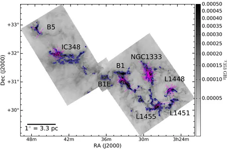
Figure 1 shows the Zari et al. (2016) τ353 GHz map of

Perseus. For simplicity, we masked out theP lanck-only regions of the map which extend beyond the Herschel

observations. The resolution of these P lanck-only re-gions are too coarse to resolve the filaments and none of our MASSES targets are located within them.

3. DATA ANALYSIS TECHNIQUES

In this section, we summarize how we measure PAs for both outflows and filaments from observations. All angles are measured counterclockwise from the north ce-lestial pole. These PAs are used to calculate the main parameter of interest,γ, which is the projected angle dif-ference between the outflows and filaments. Specifically,

γ is given by

3h24m

30m

36m

42m

48m

RA (J2000)

+30°

+31°

+32°

+33°

Dec (J2000)

B5

IC348

B1E

B1

NGC1333

L1448

L1455

L1451

1

= 3.3 pc

0.00005

0.00010

0.00015

0.00020

0.00025

0.00030

0.00035

0.00040

0.00045

0.00050

τ

35

3

G

H

z

Figure 1. τ353 GHz map of the Perseus molecular cloud (Zari et al. 2016), with magenta lines showing the directions of the outflows

measured in this study. The size of the lines only represents the direction of the outflow and not the angular extent. Thin blue contours are shown forτ353 GHz= 0.0002. These contours roughly show the boundaries of each labeled clump and correspond to a column density

ofN(H2)≈5×1021cm−2(Sadavoy et al. 2014).

where PAOut and PAFil are the PAs of the outflow and

filament, respectively. MIN indicates that we are inter-ested in the minimum of the two values in the brackets. Table3 lists the measured PAs for all outflows and fila-ments in this study.

3.1. Outflow Position Angles

We present the outflow PAs in Table3. We indepen-dently measure the outflow PAs for both the blue- and red-shifted outflows (henceforth, called the blue and red lobes). The range of the PA measurements are from –180◦ to +180◦; both positive and negative values allow one to assign the appropriate quadrant for the outflow. We also provide the combined PA, PAOut, which is

sim-ply the average of the two outflows after adding 180◦ to the lobe with the negative PA. Some entries only pro-vide measurements for one lobe because the other lobe was undetected.

In many cases (about half of the sources) we used out-flow PAs from other CO line studies in place of MASSES observations since these studies had data that are better quality and/or at higher resolution. We indicate which study provided the outflow direction for each protostar in the “Ref/Info” column of Table3. For the majority of the measured outflow PAs in this study, we made mea-surements using a methodology very similar to that used in Hull et al. (2013). We connect the peak intensity of the SMA 1.3 mm continuum observations with the peak of the integrated intensity maps for both the blue and red outflow lobes. Based on visual inspection, if the CO

line emission obviously traces the outflow cavity walls rather than the outflow centroid, we connect the contin-uum peak to a local CO maximum near the contincontin-uum rather than the absolute maximum. In cases where there are no clear local outflow maxima for one lobe, we use the PA measured by the other lobe. If no local maxima exists for both lobes and the CO only traces cavity walls, we manually measure the PA by eye. We indicate in the “Ref/Info” column of Table 3 which outflow measuring method we used. For the angles measured in this paper, a crude approximation of the uncertainty can be found by subtracting the blue outflow PA from the red outflow PA. With such an approximation, the uncertainty in the outflow PA is typically less than 10◦.

Frequently, the observed field about a MASSES tar-get overlaps with other protostellar sources, which can cause significant confusion in assigning which emission comes from which protostar. To disentangle which emis-sion belongs to which source, we used SAOImage DS9 to overlay all CO emission detected with MASSES on top of Spitzer IRAC emission (not shown). In particular, both the 3.6 and 4.5µmSpitzerbands trace the outflow cavities in scattered light and/or knots of H2 emission

3h43m00s 20s 40s 44m00s 20s 40s RA (J2000) +31°50' 55' +32°00' 05' 10' De c ( J20 00 ) Per-emb 1 3h43m00s 20s 40s 44m00s 20s 40s RA (J2000) +31°50' 55' +32°00' 05' 10' 3h43m54s 55s 56s 57s 58s 59s RA (J2000) +32°00'15" 30" 45" 01'00" 15"

30" _{[3.0, 5.0] -13.5 to 6.5 km s}−1

[6.6, 10.0] 10.5 to 48.5 km s−1

[0.013, 0.02] 0.0002 0.0004 0.0006 0.0008 0.0010 0.0012 0.0014 0.0016 0.0018 0.0020 τ 353 G Hz 3h24m40s 25m00s 20s 40s 26m00s 20s RA (J2000) +30°35' 40' 45' 50' 55' De c ( J20 00 ) Per-emb 22 3h24m40s 25m00s 20s 40s 26m00s 20s RA (J2000) +30°35' 40' 45' 50' 55' 3h25m20s 21s 22s 23s 24s 25s RA (J2000) +30°44'45" 45'00" 15" 30"

45" [8.0, 5.0] -32.9 to -0.9 km s

−1

[4.1, 5.0] 8.1 to 23.6 km s−1

[0.016, 0.02] 0.0002 0.0004 0.0006 0.0008 0.0010 0.0012 0.0014 0.0016 0.0018 0.0020 τ 353 G Hz 3h28m00s 20s 40s 29m00s 20s 40s RA (J2000) +31°05' 10' 15' 20' 25' De c ( J20 00 ) Per-emb 27 3h28m00s 20s 40s 29m00s 20s 40s RA (J2000) +31°05' 10' 15' 20' 25' 3h28m53s 54s 55s 56s 57s 58s RA (J2000) +31°14'00" 15" 30" 45" 15'00"

15" _{[5.4, 5.4] -19.5 to 1.5 km s}−1

[6.0, 6.0] 11.5 to 22.5 km s−1

[0.03, 0.05] O1 O2 0.0002 0.0004 0.0006 0.0008 0.0010 0.0012 0.0014 0.0016 0.0018 0.0020 τ 353 G Hz

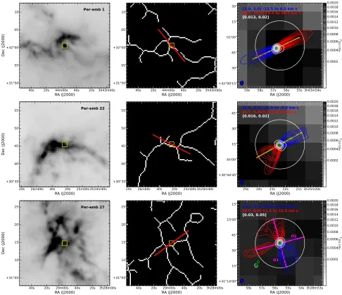
Figure 2. Figures demonstrating theFILFINDERalgorithm for Per-emb 1 (top 3 panels), Per-emb 22 (middle 3 panels), and Per-emb 27 (bottom 3 panels); other Perseus protostars can be found in the eletronic version of this paper. The left and middle panels show the τ353 GHzmaps (Zari et al. 2016) and the fitted filament skeletons fromFILFINDER(Koch & Rosolowsky 2015), respectively. The red line

in the middle panel shows the fitted PAFil,F for the protostar. The yellow squares in these two panels show the area we zoom-in for the

right panels. The right panels show theτ353 GHz overlaid with SMA red and blue CO(2–1) integrated intensity contours of the red and

blue lobes, respectively. The white contours show the SMA 1.3 mm continuum. The color-coded bracketed numbers in the top left give the first contour level followed by the contour level increment for each subsequent contour. The CO(2–1) contour levels and increments are in units of Jy beam−1_{km s}−1 _{while the continuum contour levels and increments are in units of Jy beam}−1_{. The red and blue velocity}

interval for CO(2–1) intensity integration are shown next to their corresponding contour levels. The small green circles show the location of the protostellar sources as determined at high resolution by the VLA (Tobin et al. 2016). The measured PAOutis shown as a line under

the contours, and the line is yellow if PAOutcomes from this study, and magenta if PAOutcomes from other studies (as indicated in Table 3). The white circle shows the 4800_{diameter (FWHM) primary beam of the SMA.}

to determine. Protostars surveyed by MASSES that are not presented in this paper were either not yet imaged or had confusing CO emission that did not allow for a reliable measurement of PAOut. In total, we have PAOut

measurements for 57 protostellar outflows. In Figure 1 we overlay each PAOut measurement on the Herschel

-derived τ353 GHz map. The SMA CO(2–1) integrated

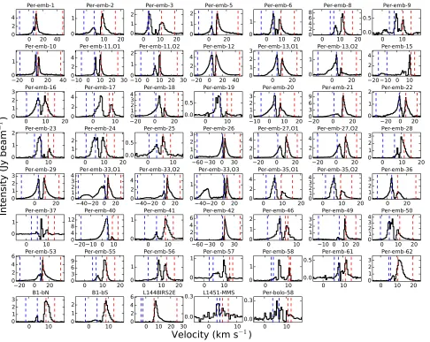
in-tensity maps for two protostars are shown in the right panels of Figure2; other sources can be found in the elec-tronic version of the paper. The average spectra within the vicinity of the protostar (i.e., within a radius of 800) is shown in Figure3.

3.2. Filament Direction

We present the filament PAs in Table 3. We deter-mine the filament directions based on Herschel-derived

τ353 GHz maps (see Section 2.2). Since extracting

fila-ments directions can sometimes depend on the method used, we use two different techniques. One technique is based on FILFINDERand the other is based on SExtrac-tor. For both techniques, we also investigate how the filament directions depend on both small and large scale optical depth characteristics.

0 20 40 02

4

Per-emb-1

0 10 20

0 1

Per-emb-2

0 10 20

01 2 Per-emb-3 0 20 0 1 2 Per-emb-5

0 10 20 0

1

Per-emb-6

0 10 20

02 46 8 Per-emb-8 0 10 0.0 0.5 Per-emb-9

−20 0 20 40 0

1

Per-emb-10

−10 0 10 20 30 0

2 4

Per-emb-11,O1

−10 0 10 20 300 1

2 Per-emb-11,O2

−20 0 20 40 0 2 4 Per-emb-12 0 20 01 2 3 Per-emb-13,O1 0 20 0 1 Per-emb-13,O2

−20−10 0 100 2

4

Per-emb-15

0 10 20

01 2 3 Per-emb-16 0 10 02 4 Per-emb-17

−200 0 20 1

2 3

4 Per-emb-18

0 10

0.0 0.5

Per-emb-19

−10 0 10 20 01

2 3

Per-emb-20

−200 0 20 3

6 9

Per-emb-21

−20 0 20 0

1

2 Per-emb-22

0 10

0 1

2 Per-emb-23

0 10 20

01 2 Per-emb-24 0 10 0.0 0.5 Per-emb-25

−60 −30 0 30 0

1 2

3 Per-emb-26

−20 0 20

0 2 4

Per-emb-27,O1

−20 0 20

0 2 4

Per-emb-27,O2

0 10 20

0 1 2 3 Per-emb-28 0 20 01 2 3 Per-emb-29

−40−20 0 20 01

2 3

4 Per-emb-33,O1

−40−20 0 20 0

2 4

Per-emb-33,O2

−40−20 0 20 0

1

Per-emb-33,O3

0 10 20

02

4 Per-emb-35,O1

0 10 20

01 23 4 Per-emb-35,O2 0 20 0 1 2 3 Per-emb-36 0 10 0 1 Per-emb-37

−20−10 0 10 0 4 8 12 Per-emb-40 0 10 0 1 Per-emb-41

−60 −30 0 30 0

2 4

6 Per-emb-42

0 10

01

2 Per-emb-46

−10 0 10 20 01

2 3

Per-emb-49

0 10 20 01

23

4 Per-emb-50

−20 0 20 0

2 4

6 Per-emb-53

0 10 20

0 3 6

9 Per-emb-55

0 10 20

0 1 Per-emb-56 0 10 0 1 Per-emb-57 0 10 0 1 Per-emb-58 0 10 0.0 0.5 Per-emb-61

0 10 20 0 1 2 3 Per-emb-62 0 10 01 2 3 B1-bN 0 10 01 2 B1-bS

0 10 20 30 0 2 4 6 L1448IRS2E 0 10 0.0 0.3 L1451-MMS 0 10 0.0 0.3 Per-bolo-58

Velocity (km s

)

Int

en

sit

y (

Jy

be

am

)

Figure 3. Average CO(2–1) spectra within a radius of 800_{from each protostar, where the protostar’s position is given in Table3. The}

velocity resolution is 0.5 km s−1_{. The vertical dashed lines show the interval ranges used to produce the integrated intensity maps in the}

right panels of Figure2. The two blue and two red lines show the integrated intervals for the blue- and red-shifted emission, respectively. These integrated intensity ranges were manually adjusted to produce the best visualization of the outflows for each source. In some cases, no outflows were found for a particular lobe, or the lobe emission was difficult to extract from the large-scale CO(2–1) emission. Note that for Per-emb-57, the dominant outflow emission is toward the southeast, more than 800 from the source’s center, and thus the spectrum poorly represents the outflow emission.

The first method extracts the filamentary structure us-ing theFILFINDERalgorithm (Koch & Rosolowsky 2015) as implemented inPYTHON. FILFINDERis unique in that it can find filaments with relatively low surface bright-ness compared to the main filaments, which is achieved by using an arctangent transform on the image. This algorithm first isolates the filamentary structure across the entire map. Then, each filament within the filamen-tary structure is made into a one-pixel-wide skeleton via the Medial Axis Transform (Blum 1967). We use the default implemented parameters in theFILFINDER algo-rithm, with the exception of the parameterssize thresh

andskel thresh, which were altered to provide the best visual fit to the actual Perseus data. Specifically, for these parameters we used the valuessize thresh= 300 and skel thresh = 100. The resolution of the obser-vations (3600) and the distance to the Perseus molecular cloud (235 pc) were also provided to the FILFINDER al-gorithm.

FILFINDER determines the filament direction via the Rolling Hough Transform (Clark et al. 2014). Unfor-tunately, the Rolling Hough Transform often performs poorly in the Perseus molecular cloud since FILFINDER

sometimes combines distinct molecular clumps as a sin-gle filamentary structure. For example,FILFINDER com-bines NGC 1333 and L1455 into a single filamentary network and measures the direction of the combined structure. We find that in most of these instances, the Rolling Hough Transform poorly estimates both the small and large scale filamentary direction. Instead of this transform, we approximate the filamentary direc-tion by fitting a line to the filamentary skeleton output from FILFINDER. To do this, we first find the closest

FILFINDER skeleton pixel to the position of the proto-star given by Tobin et al. (2016). We then extract a square skeleton map of 11×11 pixels (19800 × 19800 or

3h46m 47m 48m +32°36'42'

48' 54' +33°00'

Dec (J2000)

B5

3h43m 44m 45m +31°40'

50' +32°00' 10'

20'

_IC348

3h31m 32m 33m 34m +30°40'

50' +31°00'

10'

B1

NGC1333

0.0002 0.0004 0.0006 0.0008 0.0010 0.0012 0.0014 0.0016 0.0018 0.0020

τ

35

3

G

H

z

3h27m 28m 29m 30m 31m

RA (J2000)

10' 20' 30'

40'

NGC1333

3h27m 28m 29m

RA (J2000)

+30°00'06' 12' 18' 24'

Dec (J2000)

L1455

3h25m 26m

RA (J2000)

36' 42' 48' 54'

+31°00'

_L1448

3h24m 25m

26m

RA (J2000)

18' 24' 30'

36'

L1451

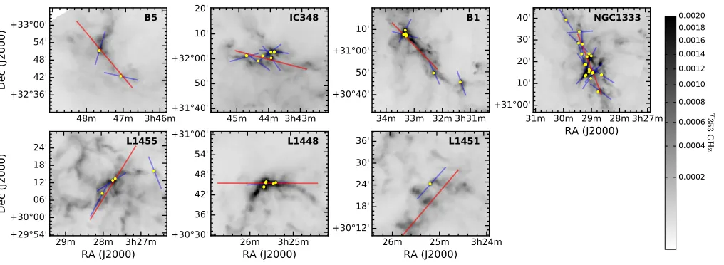
Figure 4. τ353 GHzmaps (Zari et al. 2016) of clumps within the Perseus molecular cloud. Yellow dots show the locations of protostars

with measured outflow PAs. The closest blue and red line-centers to each yellow dot represent the small and large scale direction of the filament, respectively, based on fits using SExtractor (essentially a by eye fit; see Section3.2). Lines are centered based on the centroid of the SExtractor fit. For both the blue and red lines, the length of the lines are the same angular size in each panel.

1990; Feigelson & Babu 1992) to the scatter plot of the skeleton pixels. The slope of this fitted line is then con-verted to a PA. We use an extraction of an 11×11 pixel square because we find it large enough to fit the elonga-tion of the filament, but small enough that the filament’s direction is not strongly influenced by other nearby fila-mentary structures. We have also ran the same algorithm for extracting squares of skeleton pixels that are up to∼3 times larger or smaller than 11×11 pixels, and the results in our paper are qualitatively the same. The 11×11 pixel extraction provides the best visual fits to the filaments across all sources.

Figure2 shows examples of this fitting process for two sources; other sources can be found in the electronic ver-sion of this paper. Note that the measured PA (red line in middle panels of Figure 2) are slightly off as one may measure by eye simply because nearby filament branches in the 11×11 pixel cutout of the skeleton map affects the bisector fit. In the rest of the paper, we will re-fer to this method for extracting filament directions as the “FILFINDERalgorithm.” In Table3, we provide these filament angles, PAFil,F, along with their corresponding

projected outflow-filament angle,γ_F.

Angular momentum of a protostar could possibly be inherited from filamentary structures larger than the fil-aments measured with 3600resolution. Therefore, we also make a comparison to larger scales by Gaussian smooth-ing the Zari et al. (2016) τ353 GHz maps and rerunning

the FILFINDER algorithm discussed above. Specifically, we smooth the data to resolutions of 10, 20, 30, 40, 50, and 60, where 10 is 0.068 pc, assuming a distance of 235 pc to Perseus. FILFINDER progressively finds fewer branches in the Perseus filaments when we smooth τ353 GHz maps

to these coarser resolutions. The measured projected outflow-filament angles for these resolutions are shown in Table3asγ_X0, where X0is the smoothed resolution in

arcminutes.

3.2.2. Using SExtractor for Filament Position Angles

The second method fits ellipses to the filaments via SExtractor (Bertin & Arnouts 1996), as implemented in

the Graphical Astronomy and Image Analysis (GAIA) Tool16_{. SExtractor works by fitting ellipses to the}

emis-sion data. We then adopt the position angle of the fitted ellipses as the filament PA. To measure both the large scale and small scale filamentary structure, we extract two different filament directions for each protostar. For the large scale structure, we fit a single filamentary direc-tion to the clump (i.e., the pc-scale cloud structure), and for the small scale, we fit the most localized elongated structure for the protostar. For both scales, the param-etersDetection threshold,Analysis threshold, and

Contrast parameter were adjusted for each source so that the fitted ellipse best matches the elongation as judged by the human eye. We find that no single set of values for these three parameters can fit all filaments in the Perseus cloud that is agreeable with the human eye, and thus the parameters were adjusted filament-by-filament. Therefore, this method is primarily a “by eye” determination of the filament direction with the aid of software. This method of determining the filament PA is very similar to the method used in Anathpindika & Whitworth(2008). We note that even at the small scale, the best SExtractor fit for a local filament may be the same for multiple protostars.

Figure4shows both the small and large scale filament PAs determined for each protostar using this method. The final projected outflow-filament angles using this method for both the small scale (γ_{se,S) and large scale}

(γ_{se,L) are given in Table} 3. The measured filament PAs for both of these methods can be derived fromγ_se,S

andγ_{se,L by using Equation}3and the individual PAOut

measurements.

3.2.3. Comparison of theFILFINDERand SExtractor Techniques

Both the FILFINDER and SExtractor filament-finding methods have their advantages and disadvantages. For example, the first method is completely automated, and

16

0

10

20

30

40

50

60

70

80

|

|

0

2

4

6

8

10

12

14

16

18

Nu

mb

er

of

An

gle

Di

ffe

ren

ce

s

Figure 5. Histogram showing the magnitude of the difference in the projected outflow-filament angles measured by the two methods used to find the filament orientation. γvalues for theFILFINDER

algorithm and the small scale SExtractor fits are indicated byγ_F andγ_{se,S, respectively.}

if there are multiple filamentary branches in the field, the algorithm attempts to find the best filamentary direction in a fixed area of∼0.2 pc×0.2 pc. However, filamentary branches may be considered as a contaminate, in which case the second method (the SExtractor by eye measure-ment) may more accurately determine the filamentary direction.

When comparing the two methods, the filament di-rection found with the FILFINDER algorithm are most comparable to those found at small scale with SExtrac-tor since these both measure filaments at approximately the same size scales. Figure5 shows the absolute value of the difference in the measured anglesγ_F andγ_{se,S for}

each protostar. Since PAOut for each protostar is

mea-sured the same regardless of the method used to measure the filament orientation, γ_F – γ_{se,S is equivalent to the}

difference in the measured filament directions for each technique. This histogram shows that the measured fil-ament position angles mostly agree, but in some cases, the measured filament angles for each technique vary sig-nificantly. Therefore in the following section, we present statistical comparisons to the outflows for both filament-finding techniques.

4. RESULTS

In this section, we analyze the distributions of PAOut

and γ. We note that, when we compare our empirical distributions of angles PAOut and γ to simulated data,

we favor the Anderson–Darling (AD) test (e.g.,Stephens 1974) over the Kolmogorov–Smirnov test. The AD test tends to be more powerful in detecting differences in dis-tributions than the Kolmogorov–Smirnov test, particu-larly at the tail ends of the distributions (e.g.,Hou et al. 2009;Engmann & Cousineau 2011;Razali & Wah 2011). While thep-values differ for these two tests, the overall statistical significance does not change dramatically and our conclusions remain unchanged. For the two-sample AD test, p-values near 1 imply that the two distribu-tions are likely drawn from the same distribution, while

0

20

40

60

80 100 120 140 160 180

Outflow Position Angle

0

2

4

6

8

10

12

14

Nu

mb

er

of

Ou

tflo

w

PA

s

Outflows from All Protostars

IC348

B1

NGC1333

L1448

L1451

L1455

B5

Figure 6. Stacked histogram (with 20◦ bins) of outflow PAs in the Perseus molecular cloud. Colors correspond to the clump that PAOutbelongs to.

0

20

40

60

80 100 120 140 160 180

Outflow Position Angle

0

2

4

6

8

10

12

14

Nu

mb

er

of

Ou

tflo

w

PA

s

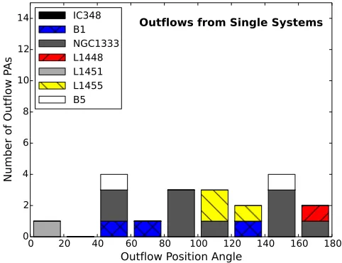
Outflows from Single Systems

IC348

B1

NGC1333

L1448

L1451

L1455

B5

Figure 7. Same as Figure6but now only considering protostars that were not identified as multiples in the VANDAM survey ( To-bin et al. 2016).

p-values near 0 imply that they are unlikely drawn from the same distribution.

4.1. Outflow Directions in Perseus

Figure 6 shows a stacked histogram of PAOut, where

the color of each stacked bar indicates the protostar’s parental clump. As with Figure 1, this figure does not show any obvious relationship between PAOut and the

the AD test givesp-values of 0.65 and 0.62, respectively. This signifies that we cannot distinguish the PAOut

his-tograms in Figures 6 and 7 from a random distribution of angles.

0 15 30 45 60 75 90

Projected

angle between outflow and filament,

(deg)

0.0 0.2 0.4 0.6 0.8 1.0

Cu

mu

lat

ive

D

ist

rib

uti

on

Fu

nc

tio

n

Random

0−20◦

70−90◦

MASSES Outflows, Herschel Filaments

Observations

Figure 8. Cumulative distribution function of the projected an-gles between outflows and filaments,γ. The red step function shows γ_Ffor this study, which measures the angle between MASSES out-flows and fittedHerschelfilaments directions using theFILFINDER

algorithm discussed in Section 3.2. The three blue lines show Monte Carlo simulations of the expected projected γ for out-flows and filaments that are 3-dimensionally only parallel (actual outflow-filament angle that is between 0 and 20◦_{), only}

perpendic-ular (70–90◦), or completely random (0–90◦).

4.2. Cumulative Distribution Functions using FILFINDER Filament Angles

While the first visual and clump regional tests did not show any obvious relationship between clump structure and protostellar outflow directions, clumps are pc-sized while filaments are about 0.1 pc in diameter (e.g., Ar-zoumanian et al. 2011). As discussed in Section3.2, we useFILFINDERto extract filament directions at the 3600 (0.04 pc) scale. These filament directions, PAFil,F, are

then compared to PAOut to determine the projected

out-flow and filament angular difference, γ_F. We plot the cumulative distribution function (CDF) of the observed

γ_F in Figure 8. To investigate whether the distribution of γ_F reflects outflows and filaments that are primarily aligned parallel, perpendicular, or at random, we per-form 3-D Monte Carlo simulations that we project onto 2-D. Specifically, we simulate the CDF of the expected projected angles in the sky for outflow-filament angles that are 3-dimensionally “only parallel” (defined as ac-tual outflow-filament angles that are distributed between 0◦and 20◦), “only perpendicular” (actual angles between 70◦ and 90◦), or completely random (actual angles be-tween 0◦ and 90◦). The expected observed (i.e., pro-jected) γ for these three Monte Carlo instances are also shown in Figure 8. Detailed information on the Monte Carlo simulations is presented in AppendixA.

Immediately evident from Figure8is that the distribu-tion ofγ_F is inconsistent with outflows and filaments that are preferentially parallel. The projected angles are also inconsistent with a purely perpendicular alignment with

0

10

20

30

40

50

60

70

80

90

γ_F

0

2

4

6

8

10

12

14

16

Nu

mb

er

of

γF

An

gle

s

IC348

B1

NGC1333

L1448

L1451

L1455

B5

Figure 9. Same as Figure 6, but now the stacked histogram is shown forγ_F. The histogram bin size is 10◦.

over 99% confidence (AD test gives a p-value = 0.0045). However, we cannot significantly distinguish the γF

dis-tribution from a disdis-tribution of randomly aligned out-flows and filaments (p-value = 0.20). Table1summarizes the statistical tests conducted on all theγmeasurements discussed in Section 3. In Figure 9, we show the dis-tribution of γ_F as a stacked histogram, with colors rep-resenting the parental clump. No obvious non-random relationship is found, regardless of the protostar’s clump location.

0 15 30 45 60 75 90

Projected

angle between outflow and filament,

(deg)

0.0 0.2 0.4 0.6 0.8 1.0

Cu

mu

lat

ive

D

ist

rib

uti

on

Fu

nc

tio

n

Paral

lel

50% Para

llel, 50% Perp endicular

100% Perpe

ndicu lar

Observations

Best Fit Bimodal Distribution

Simulated Random Distribution

Figure 10. Cumulative distribution function of the projected an-gles between outflows and filaments, γ, with the red step curve showing the empirical distribution, γF. Black dashed lines show

different mixes of projected outflow-filament angles that are 3-dimensionally parallel and perpendicular in increments of 10% (i.e., the top line is 100% parallel and 0% perpendicular, the next line is 90% parallel and 10% perpendicular, and so on). Parallel angles are defined as 3-dimensional angles drawn from a distribution be-tween 0◦and 20◦, while perpendicular angles are defined as angles drawn from a distribution between 70◦and 90◦(see AppendixA

So far, we produced simple models ofγ from outflow-filament angles that are only parallel, only perpendicu-lar, or aligned at random. As mentioned in Section 1, outflow orientation may be determined by the dominant flow direction about the filament. Therefore, a bimodal distribution of γ is possible, e.g., a mix of both parallel and perpendicular orientations.

We test different 3-dimenisonal combinations of purely parallel (again, where angles are distributed between 0◦ and 20◦) and purely perpendicular (angles between 70◦ and 90◦) outflow-filament angles via Monte Carlo sim-ulations. We consider 101 bimodal cases in increments of 1% (i.e., 100% parallel, 99% parallel and 1% perpen-dicular, 98% parallel and 2% perpenperpen-dicular, ..., 100% perpendicular). Figure10shows the CDFs of several of these bimodal distributions projected into 2 dimensions. We find that, when comparing to the observed distribu-tion γ_F, the simulated γ that is a mix of 22% parallel and 78% perpendicular maximizes the p-values for the AD test (as well as the Kolmogorov–Smirnov test). The

p-value for this case is 0.55, signifying a slightly more consistent distribution with the observedγ_F distribution than a random distribution.

This bimodal test can also constrain which mixes of parallel and perpendicular are unlikely. According to the AD test, we find that at 95% confidence,γ_F probably does not come from a bimodal distribution that is more than 39% parallel or more than 94% perpendicular. At 85% confidence, we find that theγ_F distribution does not come from a bimodal distribution that is more than 33% parallel or more than 90% perpendicular.

Other mixes ofγ distributions are also possible, such as mixes of a random distribution with perpendicular and/or parallel distributions. We do not test other dis-tribution mixes in this paper since we mainly want to show that perpendicular outflows and filaments are much more likely than parallel.

0 15 30 45 60 75 90

Projected angle between outflow and filament,

(deg)

0.0 0.2 0.4 0.6 0.8 1.0

Cu

mu

lat

ive

Di

str

ibu

tio

n F

un

cti

on

Random

0−20◦

70−90◦

36" resolution

1' resolution

2' resolution

3' resolution

4' resolution

5' resolution

6' resolution

Filament Directions Using Different Resolutions

Figure 11. Figure caption is the same as Figure 8, except with additional step curves showing the effects of smoothing the Perseus τ353 GHzmap before running theFILFINDERalgorithm described in

Section3.2. The colors indicate which resolution theτ353 GHzmap

was smoothed to in creating the empiricalγCDF.

Table 1

Anderson–Darling Testp-values

Empiricalγ p-value, compared p-value, compared Distribution with Random with Perpendicular

γF 0.20 0.0045

γ₁0 0.33 0.00085

γ₂0 0.40 0.0011

γ₃0 0.42 0.0029

γ₄0 0.49 0.00024

γ₅0 0.24 0.023

γ

60 0.59 0.00069

γ_se,S 0.74 0.00014

γ_se,L 0.64 0.0021

Anathpindika & Whitworth 0.017 0.16

γ_F, Single Protostars 0.60 0.18

γ_F, Multiple Protostars 0.20 0.011

γ_F, withTbol<50 0.53 0.021

γ_F, withTbol>50 0.18 0.075

γ_F, withτ353 GHz<0.016 0.15 0.20

γ_F, withτ353 GHz>0.016 0.27 0.0050

Note. —p-values are not shown for empiricalγdistributions compared with parallel

γdistributions because they are all extremely low in value (less than 10−9 ).

As discussed in Section3.2, we also determine filament angles by running the FILFINDERalgorithm on Perseus

τ353 GHz maps that have been smoothed to coarser

reso-lution. The resulting CDFs forγat these resolutions are shown in Figure 11. We find that the CDFs at all res-olutions are similar with each other, with the AD test

p-value 0.45 or greater when comparing any two dis-tributions. We also find consistent results between the smoothed and the non-smoothed (3600) resolutionγ an-gles. Specifically, as shown in Table 1, none of the γ

distributions extracted from the smoothedτ353 GHzmaps

can be statistically distinguished from a random distribu-tion, but all are inconsistent with projected angles from an only perpendicular and only parallel distributions.

0 15 30 45 60 75 90

Projected angle between outflow and filament,

(deg)

0.0 0.2 0.4 0.6 0.8 1.0

Cu

mu

lat

ive

Di

str

ibu

tio

n F

un

cti

on

Random

0−20◦

70−90◦

SExtractor, small scale

SExtractor, large scale

Anathpindika & Whitworth

Filaments Directions Using SExtractor Fitting

4.3. Cumulative Distribution Functions using SExtractor Filament Angles

In Figure12, we show the CDFs when using the SEx-tractor filament direction fits, which is essentially a fit by eye (see Section3.2). We find similar results for both the small-scale (i.e., fitting the closest elongated feature to each protostar) and large-scale (i.e., fitting the main part of the clump containing each group of protostars) SEx-tractor fitting as with the FILFINDERalgorithm. That is, the SExtractor fits are not inconsistent with a ran-dom distribution and are significantly inconsistent with both parallel and perpendicular angle distributions (see Table 1). Also shown in this figure are the results from Anathpindika & Whitworth (2008), which uses a simi-lar filament fitting algorithm. Unlike our results, their distribution forγ is more consistent with perpendicular (p-value of 0.17) than random (p-value of 0.017). How-ever, we caution an interpretation of the Anathpindika & Whitworth(2008)γdistribution due to several short-comings in their study, which are discussed in detail in AppendixB. We do not show the results fromDavis et al. (2009) because they do not supply any information onγ

or the filament PAs.

As in Section4.2, we also test which bimodal distribu-tion of parallel and perpendicular projected orientadistribu-tions matches the observations using SExtractor filament fits. The results are similar as those found withFILFINDER.

4.4. Cumulative Distribution Functions Based on Protostellar Characteristics

Here we investigate whether or not individual charac-teristics of the protostars themselves or their surround-ing environment affect the underlysurround-ingγdistribution. We consider the protostar’s multiplicity, the protostar’s bolo-metric temperature (Tbol), and the Zari et al. (2016)

τ353 GHz pixel value at the protostar. Both the

proto-stellar multiplicity andTbol were taken fromTobin et al.

(2016) and references therein. For multiples that were resolved with the VLA but not withSpitzer, we assign the sameTbolfor all multiples within theSpitzer-defined

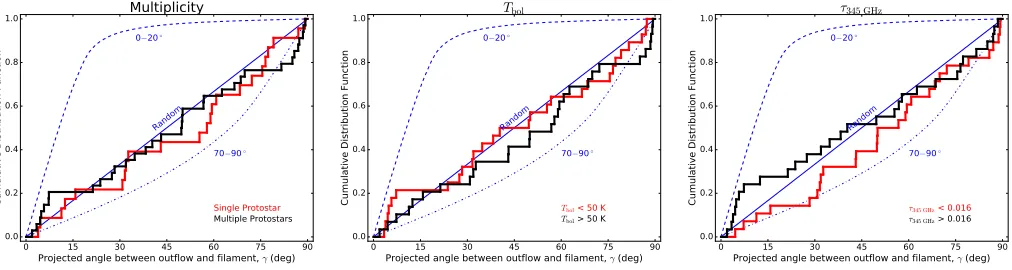
source. The left panel of Figure13shows two CDFs: one for systems that have only one known protostar within 10,000 AU and another for systems with more than one known protostar within 10,000 AU. The middle panel shows two CDFs based for protostars with Tbol above

and below 50 K, where lowerTbol indicates younger

pro-tostars. The right panel shows two CDFs based on the

τ353 GHzpixel value at theTobin et al.(2016) protostellar

location for τ353 GHz above and below 0.016. Protostars

at locations of higher τ353 GHz are more likely to be in

their natal star-forming filament. We select delimitations ofTbol = 50 K andτ353 GHz = 0.016 so that roughly half

of the sample is in each CDF. We note thatTbol= 70 K is

typically used to separate Class 0 and Class I protostars (Chen et al. 1995;Enoch et al. 2009).

Since the distribution ofγ_F angles is separated into two CDFs for each panel in Figure13, statistically differen-tiating the distributions from random and perpendicular Monte Carlo simulations is more difficult. Table1shows that none of these CDFs can be distinguished from a random distribution, and several CDFs are statistically inconsistent with perpendicular. While we only show the correspondingp-value results if we use theFILFINDER

al-gorithm, the results would be qualitatively the same if we used the filament fits from SExtractor.

We also find that the empirical CDFs in each panel are not inconsistent with each other. Specifically, thep -value between singles and multiples is 0.80, between the twoTbolbins is 0.56, and between the twoτ353 GHzbins is

0.24. The latter shows thatτ353 GHzcould possibly be the

best discriminator between two populations of γ. This would imply that protostars that are less embedded (and likely older) have outflows perpendicular to their natal filaments. Indeed, this idea is supported by the fact that higher Tbol (i.e., older protostars) are closer to the

per-pendicular curve (albeit, very slightly) than sources with lower Tbol. However, we stress that this trend is only

tentative, as it is far from being statistically significant to draw firm conclusions. A much larger sample of proto-stars would allow for a better understanding of whether or not individual protostellar characteristics affect the observedγdistribution.

5. DISCUSSION

We find that the observed distribution of the projected angle between outflow and filaments, γ, is significantly inconsistent with projected “only parallel” (angles be-tween 0◦ and 20◦) and “only perpendicular” (angles be-tween 70◦ and 90◦) angle distributions. The observedγ

distribution instead appears more consistent with a ran-dom distribution and for certain bimodal distributions of parallel and perpendicular angles. The best match for the bimodal distribution are angles that are only paral-lel 22% of the time and only perpendicular 78% of the time. These results are at apparent disagreement with Anathpindika & Whitworth(2008), but that study has a number of caveats, as explained in Appendix B. There-fore, we believe that, at least in Perseus, our results are a better representation of the actual γdistribution.

Davis et al. (2009) also found an apparently random alignment when comparing molecular hydrogen outflows to the filament/core directions in Orion, but they did not test the idea of a mixed distribution of only parallel and only perpendicular angles. Such random alignment is supported byTatematsu et al.(2016), who found that the angular momentum axes of cores in the Orion A fil-ament are random with respect to the filfil-amentary struc-ture. Our study and these studies show that protostellar outflows in both low- and high-mass star-forming regions show no preferred orientation relative to their local fil-ament. In a study that does not compare outflows an-gles to filaments, Ioannidis & Froebrich (2012) investi-gated whether outflows are perpendicular to the Galac-tic plane. Specifically, they observed molecular hydrogen outflows within part of the Galactic plane (18◦< l <30◦;

−1.5◦ < b < +1.5◦), and they also found a somewhat random distribution of outflow PAs, with a marginal preference for outflows to be aligned perpendicular to the Galactic plane.

0 15 30 45 60 75 90

Projected angle between outflow and filament, γ (deg)

0.0 0.2 0.4 0.6 0.8 1.0

Cu

mu

lat

ive

D

ist

rib

uti

on

Fu

nc

tio

n

Random

0−20◦

70−90◦

Single Protostar

Multiple Protostars

Multiplicity

0 15 30 45 60 75 90

Projected angle between outflow and filament, γ (deg)

0.0 0.2 0.4 0.6 0.8 1.0

Cu

mu

lat

ive

D

ist

rib

uti

on

Fu

nc

tio

n

Random

0−20◦

70−90◦

Tbol < 50 K

Tbol > 50 K

Tbol

0 15 30 45 60 75 90

Projected angle between outflow and filament, γ (deg)

0.0 0.2 0.4 0.6 0.8 1.0

Cu

mu

lat

ive

D

ist

rib

uti

on

Fu

nc

tio

n

Random

0−20◦

70−90◦

τ345 GHz < 0.016

τ345 GHz > 0.016

τ345 GHz

Figure 13. CDFs ofγ, binning data based on multiplicity (left), bolometric temperature (middle, an indicator of age), and optical depth (right). All CDFs use filament measurements from theFILFINDERalgorithm.

Tilley & Pudritz(2004) show that cores within filaments can form at oblique shocks, and these shocks can impart angular momentum to the core. Simulations by Clarke et al. (2017) show that filaments accreting from a tur-bulent medium have a vorticity (and hence, angular mo-mentum) that is typically parallel to filaments, which is primarily derived from radial inhomogeneous accretion. Chen & Ostriker(2014,2015) included magnetohydrody-namics in their simulations and found that for filaments forming due to converging flows, mass flows along mag-netic field lines to both the filaments and cores (which form simultaneously). For dense filaments of size-scales on order of 0.1 pc, some observations have suggested that magnetic field lines are perpendicular to the filament’s elongation (e.g., Matthews & Wilson 2000; Pereyra & Magalh˜aes 2004; Santos et al. 2016). If such fields help drive gas perpendicular to the filaments, the results from Clarke et al.(2017) suggest that this could induce a ticity parallel to the filaments. The ability for such vor-ticity to be transferred to angular momentum at the core scale or smaller is unclear, and this was not investigated byClarke et al.(2017). However, if angular momentum is inherited by the protostar in the same direction of the vorticity, we would expect the rotation of the protostar to be parallel with the filament. Indeed, simulations by Tilley & Pudritz(2004) andBanerjee et al.(2006) show that for filaments forming due to colliding flows, oblique shocks can impart net rotation parallel to the filament, which in turn can produce parallel filaments and proto-stellar rotation axes. However, numerical simulations by Whitworth et al.(1995) suggest that filaments can form via two colliding clumps, and the initial net angular mo-mentum of the system will typically be perpendicular to the filaments that form. The protostar can inherent this angular momentum, and thus its rotation axis will tend to be perpendicular to the filament. Theoretical predic-tions of rotation axes either parallel or perpendicular to the filament axes are at odds with observations at both the core (Tatematsu et al. 2016) and protostellar scales (this study).

Since filaments may be created through a variety of mechanisms, a combination of these mechanisms could cause outflow-filament alignment to appear more ran-domly aligned. Assuming the alignment is not purely random, our observations suggest that outflows are more likely to form perpendicular than parallel to the filamen-tary elongation. Unfortunately, two-dimensional

projec-tions of 3-dimensionally random and mostly perpendic-ular distributions look quite similar, making it difficult for even large samples to distinguish between the two. Moreover, the fact that the angles between outflows and filaments are neither purely parallel nor purely perpen-dicular may reflect how material is funneled toward the protostars at both the large and small scales. On large scales, Chen & Ostriker (2014) suggested that material flows along magnetic field lines, which could be mainly perpendicular to the filament along its exterior and par-allel within the interior. This mix of flows could induce a more random-like vorticity to the parental cores of the protostars.

Higher resolution simulations have explored angular momentum transfer within cores (i.e., scales _.0.1 pc). Walch et al. (2010) used smoothed particle hydrody-namic simulations of a low-mass, transonically turbu-lent core, and found that the rotation axes of protostars tend to be perpendicular to “small” filaments (diam-eters ∼0.01 pc) within cores. However, the Herschel -derived τ353 GHz maps (3600 = 0.04 pc resolution) do not

resolve these small filaments. Observations of molecu-lar line (Hacar et al. 2013, e.g.,) or continuum tracers (e.g., Pineda et al. 2011a) suggest that filaments break into smaller substructures, and therefore the initial con-ditions for protostellar rotation and collapse may be set by these smaller structures. These substructures some-times have similar elongation as their parent filaments (Pineda et al. 2011a;Hacar et al. 2013), but not always (e.g.,Pineda et al. 2010,2015). At scales of∼10,000 AU, elongated, flattened envelopes are observed to be perpen-dicular to their outflows (e.g., Looney et al. 2007). The typical size of these flattened structures and their univer-sality remains unclear. Observational surveys that probe dense structures at scales between∼0.01 to 0.1 pc can un-cover whether and at what scale an elongated structure is perpendicular with a protostar’s angular momentum axis.

small scales it is feasible that the underlying structure, turbulence, and/or multiplicity could significantly alter the initial rotation axes. While random alignment is fa-vored in some models of turbulent accretion, even models with strong magnetic fields could result in random align-ment. Mouschovias & Morton(1985) suggested that for fragments linked by strong magnetic fields, the angular momentum orientation of the fragments depends solely on the shape of the magnetic flux tubes, which can have quite irregular shapes. If fragments in filaments are in-deed magnetically linked, our study suggests that the flux tubes connecting them are indeed irregular. The-oretical simulations have begun to incorporate gravity, turbulence, magnetic fields, and outflows to study the formation of filamentary complexes (e.g., Myers et al. 2014; Federrath 2016). Such simulations can supply a more robust expectation of the observed distribution of

γ for a large sample of outflows and filaments.

6. SUMMARY

The MASSES survey observed CO(2–1) in all the known Class 0/I protostars in the Perseus molecular cloud. With these data, along with ancillary observations of CO rotational transitions, we were able to determine the outflow PAs for each protostar. We compare these angles to the filament directions based on optical depth maps derived fromHerschel (Zari et al. 2016). We find that:

1. The outflow directions are randomly distributed in the Perseus molecular cloud. This random distri-bution appears to hold regardless of parental clump of a protostar.

2. The projected angle between the outflow and fila-ment,γ, is significantly inconsistent with a “purely parallel” and a “purely perpendicular” distribution of projected angles.

3. The observed γ distribution cannot be distin-guished from a random distribution.

4. We also consider bimodal distributions, and find a slightly more consistent distribution to the ob-served gamma distribution when 22% of the pro-jected angles are parallel and 78% are perpendicu-lar. Our observations are unlikely to come from bimodal distributions that are more than ∼33% parallel or more than∼90% perpendicular.

5. Regardless of the multiplicity,Tbol (age), or

opac-ity of the individual protostars, the observedγ dis-tribution cannot be distinguished from a random distribution. However, to better test how these different parameters of the protostars affect the γ

distribution, a larger sample is needed.

We discuss the implications of the fact that outflows and filaments are neither purely perpendicular or purely parallel. We suggest that this feature could reflect the physical conditions at large or small scale. At large scale, a dominant flow direction toward cores may not exist. At small scale, the underlying structure, turbulence, and/or multiplicity could affect the angular momentum axes. Observational surveys of dust emission at scales between

∼0.01 to 0.1 pc are needed to reveal whether and how a protostar’s angular momentum axis may be related to its natal structure.

We thank an anonymous referee for thorough and help-ful reviews. I.W.S. acknowledges support from NASA grant NNX14AG96G. E.I.V. acknowledges support form the Russian Ministry of Education and Science grant 3.5602.2017. J.J.T. acknowledges support from the Uni-versity of Oklahoma, the Homer L. Dodge endowed chair, and grant 639.041.439 from the Netherlands Organisa-tion for Scientific Research (NWO). J.E.P. acknowledges the financial support of the European Research Coun-cil (ERC; project PALs 320620). The authors thank the SMA staff for executing these observations as part of the queue schedule, Charlie Qi and Mark Gurwell for their technical assistance with the SMA data, and Eric Keto for his guidance with SMA large-scale projects. The Sub-millimeter Array is a joint project between the Smithso-nian Astrophysical Observatory and the Academia Sinica Institute of Astronomy and Astrophysics and is funded by the Smithsonian Institution and the Academia Sinica. This research has made use of the VizieR catalogue ac-cess tool and the SIMBAD database operated at CDS, Strasbourg, France. This research made use of APLpy, an open-source plotting package for Python (Robitaille & Bressert 2012).

APPENDIX

A. MONTE CARLO SIMULATIONS

Many studies have used Monte Carlo simulations to show the expected observed distribution of angles of two vectors projected into three dimensions. Several of these studies (Hull et al. 2013, 2014; Lee et al. 2016; Offner et al. 2016) were specifically interested in the same pro-jected distributions we are interested in this study, i.e., the projection of angles that are 3-dimensionally purely parallel (between 0 and 20◦), purely perpendicular (70– 90◦), or completely random (0–90◦). These studies do not discuss the exact details of the Monte Carlo simula-tions. Here we discuss our Monte Carlo method, and the results are consistent with the aforementioned studies.

For our methodology, we generated N pairs of 3-dimensional vectors with each vector random about the sky. To generate a random vector, we chose a random point on the surface of a unit sphere and then connected the sphere’s origin to this point. For the purposes of Monte Carlo simulations, sampling a random point from a unit sphere that avoids biases has been well-studied (e.g., Marsaglia 1972). We outline one such way to se-lect random points on a unit sphere below, which is based onWeisstein(2017). We first selected a random angleθ

between 0 and 2πand a random numberuthat’s between –1 and 1. From random variables θ and u, we then se-lected a random point on a unit sphere at positionx,y, andz where

x=p1−u2_{cosθ (A1)}

z=u. (A3)

A unit vector between the sphere’s origin and this point is:

~v=

"_x

y z

#

(A4)

0 10 20 30 40 50 60 70 80 90

γ3D

(deg)

0 2000 4000 6000 8000 10000 12000 14000 16000 18000

Nu

mb

er

of

An

gle

s

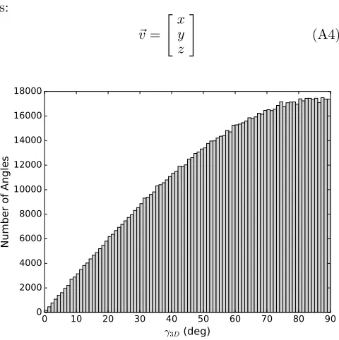
Figure 14. Histogram ofγ3Dfor a Monte Carlo simulation ofN=

106 _{vector pairs. Histogram bin widths are 1}◦_{. This histogram}

shows the approximate shape of the distribution of all possible angles between two vectors in a unit sphere.

To randomly sample from all angles within a unit sphere, we generated two random unit vectors, ~v1 and

~

v2 and measure the angle between the vectors. The

an-gle is simply

γ3D= arccos(v~1·v~2). (A5)

Since we are interested in the smallest angle created by the two intersecting vectors, we constrained γ3D to

be between 0◦ and 90◦, e.g., if γ3D is larger than 90◦,

we subtracted γ3D from 180◦. We generated N pairs

of vectors to produce N angles of γ3D. For the Monte

Carlo simulations in this paper, we chose N = 106_{. We}

show the distribution of γ3D for N = 106 via the

his-togram in Figure 14. We then mapped each γ3D angle

to a projected angle in 2D,γ, by setting one axis for the vector pair to 0 (the x-value of the vector in our code) and calculating the new angle between the vectors.

From this mapping, we can extract a range of angles from the distribution ofγ3Dand plot its correspondingγ

distribution. For this study, we were primarily inter-ested in projections for 3-dimensional angles that are purely parallel (between 0 and 20◦), purely perpendic-ular (70–90◦), or completely random (0–90◦). For the Monte Carlo sample size of N = 106 _{(equivalent to the}

number for the completely random sample size), we ex-tracted from theγ3Ddistribution∼60,000 projections for

a purely parallel sample and∼340,000 for a purely per-pendicular sample. The reason why the sample size for purely perpendicular is much larger than purely parallel is simply due to the fact that perpendicular-like angles are much more likely for two random vectors in a unit

sphere (Figure 14). Our tests show that the curve of the CDF of the Monte Carlo simulation (e.g., Figure 8) is very smooth as long as the sample size is larger than

∼20,000 projections.

B. DISCREPANCY WITH ANATHPINDIKA & WHITWORTH

As seen in Table 1 and Figure 12, Anathpindika & Whitworth (2008, henceforth in this appendix, AW08) found a distribution of projected outflow-filament angles,

γ, that favors outflows and filaments that are generally perpendicular rather than random. When comparing a random distribution to the AW08distribution of γ, the AD test p-value is 0.017, indicating a significantly non-random distribution. AW08also found that, if they as-sumedγfollows a tapered Gaussian (i.e., between 0◦and 90◦) centered at perpendicular, 72% of the time the out-flow is within 45◦of being perpendicular to the filament. To identify the PA of the outflow, AW08 connected a line between a near-IR identified YSO and the cor-responding Herbig Haro Object from Reipurth (1999). The PA of the filaments are determined from flux maps of various submillimeter surveys using SExtractor in STAR-LINK (with a visual confirmation of the PA).AW08 ac-knowledged a few selection effects that may bias their results. Specifically, they assumed that all objects have random inclinations, although adjacent sources may have correlated inclinations. Our study also suffers from this bias. AW08also suggested that they are inherently more likely to find perpendicular outflows since Herbig Haro objects are more likely to be extincted if they are coinci-dent with the filament. For these reasons, they call their conclusion not statistically robust.

AW08 also have some other disadvantages with their dataset. Their measured outflow angles rely primarily on published catalogs rather than the physical images. For about half of their sources, they interpreted multiple Her-big Haro objects emitting from a young stellar object as independent outflows. However, upon further analysis, we find this interpretation is not always accurate. As an example, Figure15shows a 3-colorSpitzer image of the outflow emanating from the SVS 13 protostellar region. TheSpitzer image shows only one obvious bipolar out-flow from the protostar (greenish 4.5µm color), and the molecular CO(1–0) line observations confirm this is a sin-gle outflow (contours in Figure15;Plunkett et al. 2013). However, AW08declared that the five HH objects asso-ciated with this outflow are five separate outflows, and each of these had a measurement ofγabove 45◦. There-fore,AW08sometimes have multiple measurements forγ

for a single outflow, which will significantly bias their re-sults toward a non-random distribution. Moreover, Fig-ure 15 shows that significantly different measurements for PAOut can be made for each Herbig Haro object for

the same outflow. The dispersion of HH objects about the outflow lobe may occur due to a precessing outflow coupled with episodic ejections (e.g., Arce & Goodman 2001;Arce et al. 2010) and/or due to the structure (e.g., clumpiness) of the ambient cloud. Therefore, measur-ing PAOut from Herbig Haro objects alone can result in

large PAOutmeasurement errors. AW08also rely on