Multiwavelength Imaging of Planetary Nebulae: Resolving & Disentangling Structure

(1)

Theses

Thesis/Dissertation Collections

10-2015

Multiwavelength Imaging of Planetary Nebulae:

Resolving & Disentangling Structure

Marcus J. Freeman

[email protected]

Follow this and additional works at:

http://scholarworks.rit.edu/theses

This Dissertation is brought to you for free and open access by the Thesis/Dissertation Collections at RIT Scholar Works. It has been accepted for inclusion in Theses by an authorized administrator of RIT Scholar Works. For more information, please [email protected].

Recommended Citation

(2)

Resolving & Disentangling Structure

Marcus J. Freeman

A dissertation submitted in partial fulfillment of the requirements for the degree of

Ph.D. in Astrophysical Sciences and Technology

in the College of Science, School of Physics and Astronomy

Rochester Institute of Technology

(3)

Ph.D. Dissertation

Multiwavelength Imaging of

Planetary Nebulae: Resolving &

Disentangling Structure

Author:

Marcus J. Freeman

Advisor:

Dr. Joel H. Kastner

A dissertation submitted in partial fulfillment of the requirements

for the Degree of Doctor of Philosophy in Astrophysical Sciences and Technology

School of Physics and Astronomy

College of Science

Approved by

Prof. Andrew Robinson Date

(4)

Astrophysical Sciences and Technologies

R

·

I

·

T

College of Science Rochester, NY, USA

The Ph.D. Dissertation of Marcus J. Freeman has been approved

by the undersigned members of the dissertation committee as satisfactory for the degree of

Doctor of Philosophy in Astrophysical Sciences and Technology.

Dr. Jan van Aardt, Committee Chair Date

Dr. Joel H. Kastner, Dissertation Adviser Date

Dr. Andrew Robinson Date

(5)

(6)

Planetary nebulae (PNe) represent the late stages of low-mass stellar evolution. The formation of the myriad of PNe morphologies involves processes that are present in many other astrophysical systems such as the wind-blown bubbles of massive stars. In this dissertation we present the results of an X-ray study of PNe, and two modeling projects that incorporate the resulting data with the goal of furthering our understanding of their X-ray properties and morphologies, and the 3D multiwavelength structure of PNe. This work expands the Chandra Planetary Nebula Survey (ChanPlaNS), which was designed to investigate X-ray emission from PNe, from 35 to 59 objects. The results from Cycle 14 Chandra observations of 24 PNe brought the overallChanPlaNSdiffuse X-ray detection rate to _∼ 27% and the point source detection rate to _∼ 36%. The detection of diffuse X-ray emission is unmistakably associated with young (.5_×103 _{yr), compact (}_R

neb.0.15

pc) PNe that exhibit closed elliptical structures and high electron densities (ne & 103 cm−3).

Utilizing the ChanPlaNS data for 14 PNe that exhibit diffuse X-ray emission, we constructed simple, spherically symmetric two-phase models using the astrophysical modeling tool, SHAPE. Our models consisted of a hot bubble and swept-up shell with the intent of investigating the X-ray morphology of these objects and the extinction caused by the swept-up shell. We compared simulated and observed radial profiles and we conclude that while most (_∼ 79%) PNe are best described by a limb-darkened X-ray morphology, this is due to nebular extinction of an intrinsically limb-brightened hot bubble structure. Expanding upon our two-phase model, we used SHAPEto generate a 3D model of the brightest diffuse X-ray PN, BD+30◦_{3639, with the model constrained}

(7)

Abstract i

Declaration v

Acknowledgements vi

List of published work vii

List of Tables viii

List of Figures ix

1 Introduction to Planetary Nebulae 1

1.1 Planetary Nebulae . . . 1

1.2 Distance . . . 3

1.3 Low-Mass Stellar Evolution . . . 5

1.3.1 Stellar Winds . . . 6

1.3.2 Wolf-Rayet Type Stars . . . 7

1.4 Shaping Paradigms . . . 8

1.4.1 Winds . . . 9

1.4.2 Tori and Disks . . . 9

1.4.3 Jets . . . 10

1.4.4 Magnetic Fields . . . 11

1.4.5 Binaries . . . 11

1.5 PNe across the spectrum . . . 12

1.5.1 Radio/Millimeter . . . 12

1.5.2 Infrared . . . 13

1.5.3 Optical . . . 14

(8)

1.5.5 X-rays . . . 14

1.6 Dissertation Synopsis . . . 15

2 X-ray Data and Analysis 17 2.1 X-rays . . . 17

2.2 X-ray Satellite Observatories . . . 18

2.2.1 Past Observatories . . . 18

2.2.2 Active Observatories . . . 20

2.3 X-ray Data Reduction . . . 22

2.3.1 Reprocessing . . . 22

2.3.2 Source detection . . . 23

2.3.3 Source event statistics and spectral extraction . . . 24

2.3.4 Output . . . 26

2.4 SHAPE: 3D Astrophysical Modeling Software . . . 27

2.5 Chapter Summary . . . 29

3 X-ray Emission from Planetary Nebulae 30 3.1 The Chandra Planetary Nebula Survey . . . 30

3.2 Observations and Data Reduction . . . 31

3.2.1 Sample: Compact (Rneb.0.4 pc) planetary nebulae within∼1.5 kpc . . . . 31

3.2.2 Observations . . . 32

3.3 Results . . . 34

3.3.1 Cycle 14 detections of X-rays from PNe . . . 36

3.3.2 PNe displaying diffuse X-ray emission . . . 37

3.3.3 PNe displaying point-like X-ray emission at central stars . . . 39

3.3.4 X-ray nondetections . . . 40

3.4 Discussion . . . 42

3.4.1 Diffuse X-ray emission from [WR]-type CSPNe . . . 42

3.4.2 Diffuse X-ray emission and PN size, age, and electron density . . . 45

3.4.3 Binary detections/nondetections . . . 46

4 Modeling Diffuse X-ray Emission of Planetary Nebulae 57 4.1 Introduction . . . 57

4.2 Target CSPNe . . . 59

4.3 The Two-Phase PNe Toy Model . . . 61

4.4 Data analysis . . . 64

4.4.1 Toy model set-up . . . 64

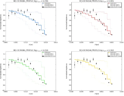
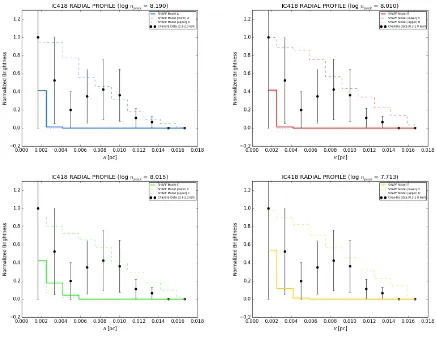
4.4.2 X-ray Radial Emission Profiles (REPs) . . . 66

4.4.3 Goodness-of-fit . . . 69

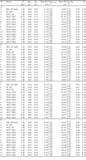
4.5 Results . . . 70

4.5.1 PNe with Poor Photon Statistics . . . 72

4.5.2 Comparison with the Frew Catalog . . . 72

(9)

4.6 Discussion . . . 76

4.6.1 Limb-Brightening vs -Darkening . . . 76

4.6.2 Swept-up Shell Density Distribution . . . 77

4.6.3 CSPNe and Nebular Extinction . . . 78

4.7 Normalized NH Estimates . . . 80

4.7.1 Emission Line Diagnostics . . . 80

5 A Multiwavelength 3D Model of BD+30◦3639 124 5.1 Introduction . . . 124

5.2 Observations and Data . . . 126

5.2.2 Infrared . . . 131

5.2.3 Optical . . . 140

5.2.4 X-ray . . . 142

5.3 Morpho-kinematic Reconstruction . . . 144

5.3.1 Optical . . . 145

5.3.3 Infrared . . . 149

5.3.4 X-ray . . . 151

5.4 Results . . . 152

5.4.1 Optical . . . 157

5.4.2 Infrared . . . 161

5.4.4 X-ray . . . 172

5.5 Re-orienting BD+30 . . . 172

5.5.1 NGC 7027 . . . 174

5.5.2 NGC 6720 . . . 176

5.5.3 NGC 3132 . . . 177

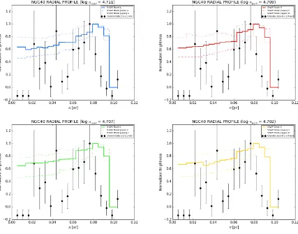
5.5.4 NGC 40 . . . 178

5.6 Summary . . . 180

6 Summary and Future Work 183 6.1 Investigating X-ray emission . . . 183

6.2 Unveiling diffuse X-ray morphology . . . 184

6.3 Modeling BD+30 . . . 185

6.4 Future Work . . . 187

6.4.1 Expand theChanPlaNS Sample . . . 187

6.4.2 Flesh Out the Toy Model . . . 188

6.4.3 Refine the BD+30 3D Model . . . 188

6.4.4 Further 3D Modeling Using AstroBEAR . . . 189

(10)

I, MARCUS J. FREEMAN (“the Author”), declare that no part of this dissertation is substan-tially the same as any that has been submitted for a degree or diploma at the Rochester Institute of Technology or any other University. I further declare that this work is my own. Those who have contributed scientific or other collaborative insights are fully credited in this dissertation, and all prior work upon which this dissertation builds is cited appropriately throughout the text. This dissertation was successfully defended in Rochester, NY, USA on ...

Modified portions of this dissertation have previously been published by the Author in peer-reviewed papers appearing in The Astrophysical Journal (ApJ):

(11)

As with any great project, it is impossible to conquer anything alone. I’d like to acknowledge NASA, Chandra X-ray Center, the Laboratory for Multiwavelength Astrophysics, and the Astro-physical Sciences and Technology program at RIT for providing me with funding for this project. I would also like to thank my advisor, Joel Kastner, who never lost faith in me throughout my various projects, and always managed to find time to work through whatever problems came up.

(12)

1. The Chandra Planetary Nebula Survey (CHANPLANS). II. X-Ray Emission from Compact Planetary Nebulae.

(13)

3.1 Planetary Nebulae within 1.5 kpca _{Observed by} _Chandra _{. . . 33}

3.2 Log of Chandra Observations . . . 34

3.3 Planetary Nebulae X-ray Point Source Characteristics . . . 35

3.4 Planetary Nebulae: Chandra X-ray Detection Statistics . . . 36

4.1 ChanPlaNS PNe within 1.5 kpca _{with Diffuse X-ray Emission} _{. . . 59}

4.2 SHAPE Toy Model Physical Parameters . . . 71

4.3 Electron Density Estimates via Various Methods . . . 81

5.1 Observations of BD+30 Reported in the Literature . . . 128

5.2 Observations of BD+30 used for SHAPE Modeling . . . 145

(14)

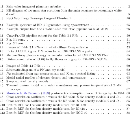
1.1 False color images of planetary nebulae . . . 2

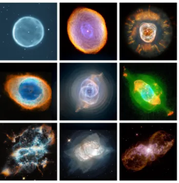
1.2 HR diagram of low mass star evolution from the main sequence to becoming a white dwarf . . . 5

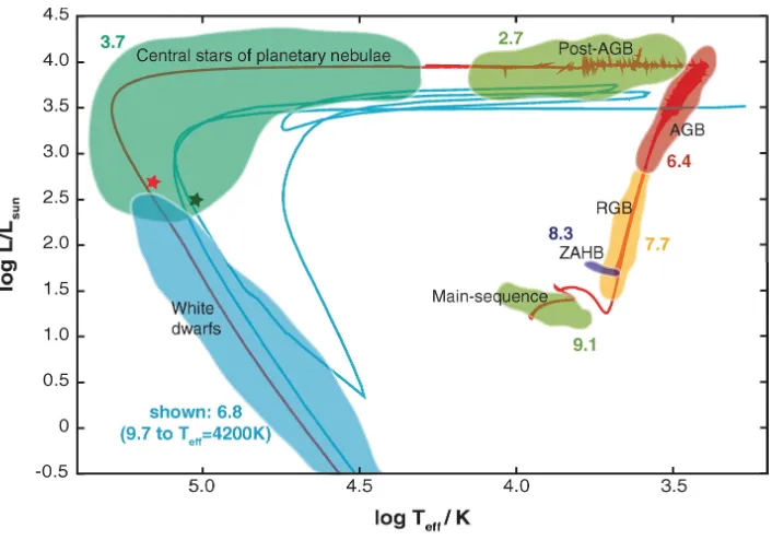
1.3 ESO Very Large Telescope image of Fleming 1 . . . 10

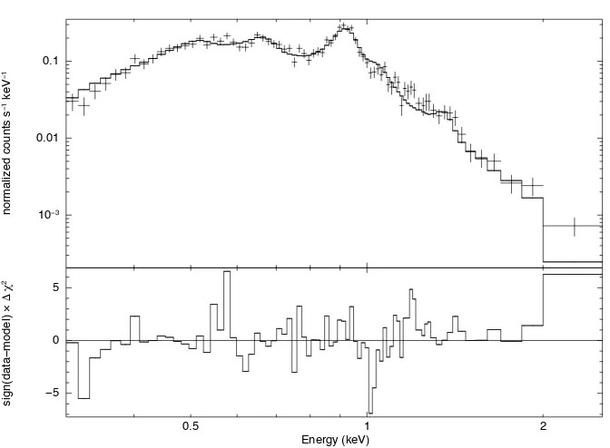
2.1 Example spectrum of BD+30 generated using specextract . . . 25

2.2 Example output from the ChanPlaNSreduction pipeline for NGC 3918 . . . 26

3.1 ChanPlaNSpipeline output for the Table 3.1 PNe . . . 50

3.1 Fig. 3.1 cont. . . 51

3.1 Fig. 3.1 cont. . . 52

3.2 Images of Table 3.1 PNe with which diffuse X-ray emission . . . 53

3.3 Plots of CSPN Teff vs. PN radius for all ChanPlaNSobjects . . . 54

3.4 Median X-ray photon energy vs. nebular radius for all ChanPlaNSPNe . . . 55

3.5 Distance and ratio of [O iii] to Hβ fluxes vs. logne forChanPlaNSPNe . . . 56

4.1 Images of Table 4.1 PNe . . . 60

4.2 Schematic diagram of a PN and toy model . . . 62

4.3 NH estimated fromcHβ measurements and X-ray spectral fitting . . . 63

4.4 Model radial profiles of electron density and temperature . . . 65

4.5 Swept-up shell density models . . . 67

4.6 Thermal plasma model with solar abundances and plasma temperature of 2 MK from xspec. . . 67

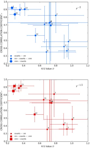
4.7 Morrison & McCammon(1983) photoelectric absorption model of X-rays by the ISM. 68 4.8 Cross-correlation coefficientr versus the KS valueDfor density models Aand B . . 84

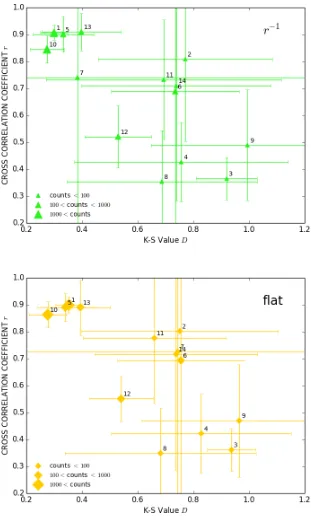
4.9 Cross-correlation coefficientr versus the KS valueDfor density models C and D . . 85

4.10 Best fit REP for the four density models used for BD+30 . . . 86

4.11 Best fit REP for the four density models used for IC 418 . . . 87

[image:14.612.91.541.285.681.2]

(15)

4.13 Best fit REP for the four density models used for NGC 1501 . . . 89

4.24 Map of our sample PNe including estimated column density . . . 100

4.25 EstimatedNH compared to distance for modelsA and B. . . 101

4.26 EstimatedNH compared to distance for modelsC and D . . . 102

4.27 Nebular density versusFrew (2008) nebular density for density modelsAand B . . 103

4.28 Nebular density versusFrew (2008) nebular density for density modelsC and D . . 104

4.29 Nebular density versus shell thickness ∆R for density models A and B . . . 105

4.30 Nebular density versus shell thickness ∆R for density models C and D . . . 106

4.31 Nebular densityne versus radiusR fbased on Frew(2008) . . . 107

4.32 Nebular densityne versus radiusR for density models A and B . . . 108

4.33 Nebular densityne versus radiusR for density models C and D . . . 109

4.34 Nebular densityne versus nebular age for density modelsA and B . . . 110

4.35 Nebular densityne versus nebular age for density modelsC and D . . . 111

4.36 EstimatedNH vs. NHdetermined from cHβ for density models Aand B . . . 112

4.37 EstimatedNH vs. NHdetermined from cHβ for density models C and D . . . 113

4.38 EstimatedNH andR for density models A and B . . . 114

4.39 EstimatedNH andR for density models C and D . . . 115

4.40 EstimatedNH vs. NHdetermined from X-ray spectra for density models A and B . 116 4.41 EstimatedNH vs. NHdetermined from X-ray spectra for density models C and D . 117 4.42 Normalized nebular densityne versus radiusR for density models Aand B . . . 118

4.43 Normalized nebular densityne versus radiusR for density models C and D . . . 119

4.44 Normalized nebular density versus Frew (2008) nebular density for density models A and B . . . 120

4.45 Normalized nebular density versus Frew (2008) nebular density for density models C andD. . . 121

4.46 Ionized mass versus Frew(2008) ionized mass for density modelsA andB . . . 122

4.47 Ionized mass versus Frew(2008) ionized mass for density modelsC and D . . . 123

5.1 Composite HSTand Chandra (blue emission) image of BD+30◦3639 . . . 125

5.2 20 and 6 cm images of BD+30; Fig. 2 from Basart & Daub(1987). . . 126

5.3 6 and 2 cm images of BD+30; Fig. 1 from Masson (1989). . . 127

5.4 2.6 and 1.3 mm images of BD+30; Fig. 1 from Bachiller et al.(2000). . . 127

(16)

5.6 21 cm contour plot of BD+30, from Taylor et al.(1990) . . . 130

5.7 CO bullet image of BD+30 showing the velocity of both components; Fig. 1 from Bachiller et al.(2000). . . 130

5.8 Mid-IR contour maps of BD+30; Fig. 1 from Bentley et al.(1984). . . 132

5.9 Mid-IR contour maps of BD+30; Fig. 1 from Hora et al.(1993). . . 133

5.10 Radial profiles of mid-IR lines of BD+30, fromHora et al. (1993) . . . 134

5.11 Mid-IR images of BD+30, fromMatsumoto et al. (2008) . . . 135

5.12 Band ratio images for BD+30, fromMatsumoto et al. (2008) . . . 136

5.13 33.6µm image of BD+30; Fig. 1 fromGuzman-Ramirez et al. (2015). . . 137

5.14 H2 torus contours over image of BD+30; Fig. 1 from Shupe et al. (1998). . . 138

5.15 H2 torus channel maps, from Shupe et al.(1998) . . . 138

5.16 H2 torus and CO bullet contours of BD+30; Fig. 3 from Bachiller et al.(2000). . . . 139

5.17 Hα image of BD+30; Fig. 2 from Harrington et al.(1997). . . 139

5.18 [Nii] and [Oiii] position-velocity diagrams of BD+30; Fig. 2 fromBryce & Mellema (1999). . . 141

5.19 ROSAT X-ray image of BD+30 at 0.059-0.12 keV; Fig. 1 fromKreysing et al.(1992). 142 5.20 Chandra X-ray image of BD+30 at 0.3 to 2.0 keV; Fig. 2 from Kastner et al. (2012). 143 5.21 HST images of Hα, [Nii], and a ratio image of Hα/[N ii] . . . 146

5.22 Radial profiles of optical emission features: Hα, Hβ, [Oiii], [N ii], [S ii], and [Siii] . 146 5.23 [Oiii] and X-ray East-West radial profiles. . . 151

5.24 Unabsorbedvapec X-ray emission model from xspecfit to BD+30 Chandradata. . 153

5.25 SHAPE model of the [O iii], [N ii], and Hα structure of BD+30. The green mesh represents [O iii] emission, the blue represents the [N ii] and Hα emission, and the navy blue mesh represents the halo of scattered optical light around BD+30. . . 154

5.26 SHAPEmodels of the [O iii] structure of BD+30 . . . 155

5.27 [Oiii] PV diagrams from Bryce & Mellema (1999) and SHAPE . . . 156

5.28 SHAPEmodels of the [N ii] structure of BD+30 . . . 158

5.29 [Nii] PV diagrams, fromBryce & Mellema (1999) andSHAPE . . . 159

5.30 SHAPEmodels of the [N ii] structure of BD+30 . . . 160

5.31 SHAPEmodels of the [Ne ii] and 11.2µm PAH structure . . . 161

5.32 SHAPEmodels of the 8.6 µm PAH structure of BD+30 . . . 162

5.33 SHAPEmodels of the 10.5 µm continuum structure of BD+30 . . . 163

5.34 SHAPEmodels of the H2 “torus” of BD+30 . . . 164

5.35 Shupe et al. (1998) and SHAPEchannel maps of the H2 structure surrounding the main nebula of BD+30 . . . 166

5.36 SHAPEmodels of the 33.6 µm silicate dust envelope of BD+30 . . . 167

5.37 SHAPEmodels of the CO bullets of BD+30 . . . 168

5.38 SHAPEmodels of the CO bullets of BD+30 overlaid with the H2 regions . . . 169

5.39 SHAPEmodels all of the radio emission regions of BD+30 . . . 170

5.40 SHAPEmodels of the 6 cm emission of BD+30 . . . 171

5.41 SHAPEmodels of the X-ray emission of BD+30 . . . 173

(17)

5.43 HSTHαimage of NGC 6720 compared with the basic render and physical render of BD+30 . . . 176 5.44 HSTHαimage of NGC 3132 compared with the basic render and physical render of

(18)

INTRODUCTION TO PLANETARY NEBULAE

1.1

Planetary Nebulae

As the near-end stages of intermediate mass (_∼1-8 M) stars, planetary nebulae (PNe) serve as

windows into the evolution and the chemical enrichment of the universe. Throughout the progenitor star’s journey up the asymptotic giant branch (AGB), it continuously sheds mass at rates from

∼ 10−7 _{to 10}−5 _M

yr−1 through a dusty, molecule-rich stellar wind (vw ∼ 10−30 km s−1).

Once helium has been exhausted in the core of the AGB star, it sheds its tenuous outer layers, revealing the compact core. The fast wind (vw'500-1500 km s−1) of the central star collides with

the previously ejected AGB wind, compressing it into a shell. As the newly revealed core evolves towards a white dwarf (WD), the effective temperature of its observable photosphere increases, and when its temperature passes 30 kK its UV radiation becomes strong enough to ionize the surrounding material, creating the PN that we are familiar with. The nebula continues to expand at a rate of ∼ 40 km s−1 _{and remains visible for 1-3}_×₁₀4 _{years before it begins to fade as the}

central star cools (Jacob et al.,2013).

Models of the formation of PNe (Kwok et al.,1978;Schmidt-Voigt & Koppen,1987;Marten &

(19)

[image:19.612.125.492.144.518.2]

(20)

their structure is strongly impacted by interacting stellar winds (ISW). From the assumption of isotropic winds in these models, we expect PNe to be spherical, but in actuality, spherical nebulae are the exception and not the rule (De Marco,2009). Hubble Space Telescope (HST) observations of a variety of PNe have revealed that the structures of PNe are not so simple, as seen in Fig. 1.1. The shapes of PNe range from multiple-shelled ellipsoids to tight-waisted bipolar structures with large lobes, and still others that feature multipolar outflows and extremely asymmetrical structures. The menagerie of PNe optical emission line morphologies demonstrates that the formation of PNe is far more complicated than the original ISW model predicts. A modified model from Kahn & West (1985) included an aspherical mass distribution to account for axisymmetric and bipolar nebulae. This generalized interacting stellar winds (GISW) theory turned out to also conflict with observations and became a subject of controversy (Balick & Frank,2002).

More advanced modeling coupled with better observations has since provided a better under-standing of the physical structures of PNe, and opened up the field of shaping mechanisms from winds to jets, disks, and the most popular hypothesis, binaries (Frank et al.,1993). PNe remain a confounding set of objects that require further investigation. There are plenty of mysteries yet to solve, such as the role of the central stellar engine and binary companions in shaping the overall 3-dimensional structure and whether or not there exists a common evolutionary model as proposed by the ISW.

1.2

Distance

We know of over 3400 PNe in the Milky Way, but given the density of PNe in the solar neighbor-hood (_∼50 kpc−3_;_{Cahn & Amd}_,₁₉₇₈_;_Frew_,₂₀₀₈_{), we expect the true number to be much higher.}

(21)

is compounded with a lack of well constrained distance measurements to PNe.

Currently, primary distance measurements that have uncertainties<10% only exist for less than one percent of all of the observed Galactic PNe (Frew et al.,2015). This results in the calculation of distances to most PNe based on statistical measurements, and depending on the method can result in varying distances from one paper to the next (Golovatyi & Demchyna,2014;Zijlstra,2015;

Frew et al.,2015). A variety of approaches have been proposed to determine PNe distances based

on a plethora of different assumptions. For example, the Shklovsky method assumed a constant ionized mass for the PN shell (Minkowski & Aller, 1954; Shklovsky, 1956), which then could be used in conjunction with mean density estimates from [O ii] or [S ii] observations. This proves to be problematic given that the ionized mass within a PN is not constant throughout its lifetime, resulting in over and underestimates for young and old PNe respectively.

Alternatively, assuming a variable mass, the optical thickness of the nebula can be related to the total ionized mass. The optical thickness is inferred from the 5 GHz radio density and then related to the mass, which can be related to the size (Daub, 1982). This same method was tweaked to assume a continuous function of linear radius and use the surface brightness (Maciel

& Pottasch,1980;Pottasch,1980), or the brightness temperature to estimate the distance (Zhang,

1995;Phillips,2002,2004a).

Another method examined PNe that were evolving with constant luminosity and were expected to have similar absolute bolometric magnitudes, and similar central stars with masses close to 0.6 M. With the star’s mass and a determination of the stellar temperature, the absolute magnitude

could be calculated and compared with the apparent magnitude from observations, leading to a distance measurement (Phillips, 2005). Still others made more specific assumptions, such as the angular size of the waist of all Type I bipolar PNe are the same, or use the angular diameter of the He II Str¨omgren zone (Phillips,2004b). The latter method can only be applied to optically thick PNe.

(22)

Gaia, we will be able to obtain primary distance measurements to many of the Galactic PNe. More accurate distance measurements will lead to better calibrated physical parameters such as radius, mass, luminosity, age of the nebulae, luminosity and mass of the central stars of the PN (CSPNe), and PNe distribution. These parameters are essential for understanding the evolution of PNe, as well as the evolution of the galaxies they reside in. For the purposes of this dissertation, we assume distances determined via the Hα surface brightness - radius (SHα-r) relation which makes use of

the Hα flux, angular size, and reddening toward the PNe to determine the distance (Frew et al.,

2015). Specifically, we assume distance values fromFrew (2008).

[image:22.612.131.484.326.573.2]

1.3

Low-Mass Stellar Evolution

Figure 1.2: Schematic Hertzsprung-Russell (HR) diagram illustrating low mass star evolution from the main sequence to becoming a white dwarf, from (Herwig,2005).

For massive stars (>8 M), the final stages of their evolution results in a violent eruption in

(23)

will evolve to become PNe through less explosive means, with the central star eventually becoming a white dwarf. Most of the star’s life is spent on the main sequence where it burns hydrogen (Fig. 1.2). Low mass stars spend the bulk of their lives here (1-10 Gyr) burning hydrogen in the core, which keeps the star in hydrostatic equilibrium, where radiation pressure outward from the fusion process balances the inward gravitational pressure.

The star eventually ceases hydrogen fusion in its core, resulting in gravitational collapse which contracts the core and heats it up. Hydrogen continues burning in a shell around the helium core and radiation pressure begins to drive the stellar envelope outward, cooling the star and making it redder and brighter. This stage marks the beginning of the red giant phase. As hydrogen burning continues, more helium is deposited into the core, and contraction continues, leading to rising core temperatures. Eventually the core heats to 108_{K and begins to fuse helium via the Triple-}_α_process.

The ignition of this core burning process is called the Helium Flash, and marks the end of the red giant phase as the star begins to get hotter and bluer, moving horizontally across the HR diagram (Fig. 1.2). Both hydrogen and helium burning continue, building up carbon and oxygen in the core. Once all of the helium is spent in the core, fusion ceases again and there is nothing to balance against gravitational pressure, resulting in another phase of of core collapse. As the core collapses it heats up, however the core temperature is never high enough to ignite carbon fusion, resulting in a degenerate core of carbon and oxygen. Surrounding this core is a shell of helium and another shell of hydrogen. This is where the star begins to ascend the asymptotic giant branch (AGB), which marks the crucial final stage before the creation of the PN (Herwig,2005).

1.3.1 Stellar Winds

(24)

and helium burning. The dust transfers momentum to the enriched gas and carries it away in a wind which has a speed on the order of 10s of km s−1 _{and at the upper part of the AGB leads to}

mass loss rates up to Myr−1. The star loses a significant fraction of its mass this way, up to 80%,

leading to the loss of the stellar envelope and the end of the AGB phase.

The central core continues to contract under gravitational pressure and increase in temperature as it evolves towards becoming a WD. With the increase in temperature comes an increase in UV radiation, which penetrates into the AGB wind, ionizing the ejecta and creating the PN. As the radius of the central star decreases, the escape velocity increases, resulting in a faster stellar wind, with velocities ranging from 500 to 1500 km s−1_{. The region closest to the central star is dominated}

by the unencumbered, fast wind. This wind plows into the previously ejected material in the slower AGB wind, compressing it and forming it into a thin shell. The collision of the fast wind with the AGB ejecta results in shocks that heat the fast wind gas to temperatures > 106 _{K, forming a}

“hot bubble” capable of producing soft X-rays (0.3∼1 keV). The hot bubble and swept-up shell are separated by a contact discontinuity, across which heat conduction can occur, which may be responsible for lowering the temperature of the hot bubble from predicted values of _∼ 107 _{K to}

observed values of _∼106 ₍_{Steffen et al.}_,₂₀₀₈_;_Toal´_{a & Arthur}_,₂₀₁₄_).

The pressure from the hot bubble and the fast wind expand the PN at a rate of _∼ 40 km

s−1 ₍_{Jacob et al.}_, ₂₀₁₃_{). As the nebula expands the central star continues to heat up, towards}

temperatures of _∼ 100 kK. Once the star can no longer contract it begins to cool down and becomes a WD. At this time, the PN has expanded and become more diffuse, becoming optically thin to UV radiation, and eventually fades away.

1.3.2 Wolf-Rayet Type Stars

There exists a subclass of central stars of PNe that are H-deficient and exhibit fast stellar winds (vw &103 km s−1) that result in high mass-loss rates (&10−6 M yr−1). Typically this subclass

(25)

low mass WR stars is identified as [WR]-type and is divided into three different types: the oxygen type [WO] , the carbon type [WC], and the nitrogen type [WN] (sometimes supplemented by an intermediate [WN/WC] classification;van der Hucht et al.,1981;DePew et al.,2011).

Multiple evolutionary paths are theorized for these stars. One theory suggests that the formation of H-deficient [WR] stars is based on the timing of the thermal pulse via the Asymptotic Giant Branch Final Thermal Pulse (AFTP), the Late Thermal Pulse (LTP) or the Very Late Thermal Pulse (VLTP). The first serves as the finale to the AGB phase, while the LTP occurs after the star has left the AGB but continues to burn hydrogen. Finally, the VLTP occurs when the star is already beginning to cool along the WD evolutionary track (Herwig,2001). Alternatively, [WR] stars are theorized to form from binary interactions, possibly being the product of a binary merger

(De Marco & Soker,2002;De Marco,2008;Hajduk et al.,2010).

Given the similarities to their more massive cousins, which produce wind-blown bubbles of their own (Toal´a & Arthur, 2011b; Toal´a et al., 2012;Zhekov & Park, 2011;Zhekov, 2014), PN around [WR]-type central stars are expected to share similar traits. The higher mass loss and wind speeds are expected to result in more pronounced limb-brightened morphologies, as the much higher wind from the [WR] star sweeps up the previous AGB wind. This also has been proposed for the diffuse X-ray morphologies for both WR and [WR]-type stars (Wrigge et al., 1994; Wrigge,1999;Wrigge

et al.,2005;Toal´a et al.,2012).

1.4

Shaping Paradigms

Originally the notion was that PNe formed from a sudden mass-loss event much like supernovae, but modeling and observations since then has proven that not to be the case (Kwok et al., 1978;

Sch¨onberner & Steffen, 2003). A variety of methods have been proposed for the generation of

(26)

1.4.1 Winds

Previously we discussed how the wind of the AGB star and the central star work together to create a PNe, however this was under the assumption that such winds are homogeneous and isotropic. While there do exist PNe that appear to fit this configuration (e.g. Abell 39, Fig. 1.1, top left), most PNe do not exhibit such well defined spherical structures. If the AGB wind is inhomogeneous and has clumpy structure, instabilities can form, resulting in asymmetrical features. Such structures are found in the circumstellar envelopes of AGB stars (e.g. IRC+10216;Le˜ao et al.,

2006), and could lead to non-uniform density distributions that result in multipolar nebulae (Steffen

et al.,2013). Additionally, if the central star were to have a binary companion, a secondary wind or

accretion onto the companion could create spiral-like structures. Such structures have been seen in AGB stars like R Scl (Maercker et al.,2012), which could explain some of the spiral-like filamentary structures seen in PNe like the Saturn Nebula.

1.4.2 Tori and Disks

(27)

Figure 1.3: ESO Very Large Telescope image of Fleming 1. The outer regions of this nebula shows symmetric jet structures indicative of a binary at its heart. (Credit: ESO/H. Boffin)

1.4.3 Jets

An inhomogeneous wind should result in asymmetrical PNe more often than axisymmetrical nebulae. Jets could be responsible for the creation of bipolar nebulae that exhibit a well defined, collimated structure. An alternative launching mechanism for the AGB shell could be the launching of a jet from within the stellar envelope. Such a jet would be launched along the poles of the star, accelerating the polar material outward faster than the equatorial material (Akashi & Soker,2013). This would result in a highly elliptical or bipolar nebula similar to Fleming 1, which shows evidence for a jet (Fig. 1.3). The jet structure of Fleming 1 has a axisymmetric, spiral-like structure with minor oscillations in it, which are attributed to a central binary (Boffin et al., 2012). Other axisymmetic structures and disturbances could be the result of the precession of the jet after the formation of the nebula (Sahai & Trauger,1998;Bujarrabal et al.,2001).

Jet structures are not often visible in many PNe with bipolar structures. Spectroscopic obser-vations have revealed high velocity outflows at speeds ∼100 km s−1 _{in several PNe, which serves}

(28)

clumps forming along the flow. Clumps like these are seen in NGC 6302, suggesting that a jet may have played some role in its formation (Akashi & Soker,2013).

1.4.4 Magnetic Fields

Collimation of bipolar nebulae may also be explained by the ejection of ionized material along magnetic field lines. Stars are expected to have magnetic fields during their main sequence lifetime, and these fields can cause accretion or ejection of material. A remnant magnetic field from the time that the central star spent on the main sequence could be responsible for some of the axisymmetric morphologies seen in PNe. Alternatively, this magnetic field could be produced as a result of a rapidly rotating stellar core within a slowly rotating envelope, resulting in the creation of a dynamo and a corresponding magnetic field (Jordan et al.,2012)

Models of dynamo generation from single and binary stars by Nordhaus et al. (2007) showed that if certain conditions are met, single stars could generate necessary magnetic fields, though common envelope binaries are far more likely to produce such fields. The addition of a secondary star results in additional energy and momentum which can boost the magnetic field. Magnetic fields up to 1 G have been measured, via polarization of radio maser emission, in the envelopes of AGB stars, and on the order of a few mG in proto-PN (Vlemmings, 2007, and refs. therein). However, surveys searching for magnetic fields emanating from the central stars of PNe have only found a few with detectable fields, of which only one is a suspected binary (Leone et al., 2011,

2014).

1.4.5 Binaries

The shapes of PNe were once exclusively linked to post-AGB stages of evolution, but it is becoming more and more apparent that the AGB phase may have a larger impact on the eventual evolution of the PN. Many AGB stars are expected to have companion stars, which is expected to impact not only the evolution, but the morphology of the subsequent PN. This Binary Hypothesis

(29)

by accreting material to form a jet or a disk, or adding extra energy to the system and a stronger magnetic field, binaries play an important role in the evolution of PNe.

It is well known that most stars form in pairs, which further supports this hypothesis. Obser-vations of AGB stars have found many with companions that have already begun to play a role in the deformation of the stellar envelope (Le˜ao et al.,2006;Mayer et al.,2014). Binary companions can also hide themselves by falling into the envelope of the central star. This common envelope binary is expected to accelerate the loss of the AGB envelope by injecting additional energy and momentum. It is in this phase of evolution that jets can form and launch the stellar envelope away from the binary (Soker,2004; Nordhaus et al.,2007;Tocknell et al.,2014;De Marco et al.,2015). As a result of the common envelope phase, the orbit of the core of the AGB star and the com-panion star shrinks, and in some cases can lead to coalescence. When this happens, the comcom-panion star disappears, leaving behind a single star. The only evidence of a companion ever existing is believed to be within the nebula itself. Not only does the morphology inform us of this, but also the chemical composition of the central star. This is how [WR]-type central stars are believed to have formed (De Marco & Soker,2002;De Marco,2008;Hajduk et al.,2010).

1.5

PNe across the spectrum

The interesting morphologies of PNe are not limited to the optical emission line observations. PNe have been observed across the electromagnetic spectrum and have revealed complicated struc-tures at every wavelength. Being able to observe PNe at a range of wavelengths is crucial for understanding their evolution, from their past to their possible future.

1.5.1 Radio/Millimeter

(30)

cm hydrogen line shows extended halos that surround nebulae and represent the gas previously ejected by the AGB star. Molecular emission from CO is also associated with shells around many PNe, but there are also cases that reveal atypical distributions of CO in the form of bullets or high velocity outflows (see Chapter 5). Radio observations have proven useful for determining electron temperatures within nebulae and the level of intervening interstellar extinction (Terzian,1968).

1.5.2 Infrared

The infrared (IR) part of the spectrum probes many complex dust and gas features within the nebula. Far-IR observations reveal large amounts of mass ejected at earlier stages of the central star’s evolution that surround the main nebula. In particular, most of the mass of the nebula is expected to be found in dust in this wavelength regime. The Herschel Planetary Nebula Survey (HerPlaNS) investigated 11 PNe at wavelengths longer than 51 µm to investigate the spatial distribution of electron density, temperature, and elemental abundances. These data can provide insight into the progenitor star’s mass loss history and the molecular makeup of such nebulae (Ueta

et al.,2014;Aleman et al.,2014).

In the mid-IR, observations typically reveal emission from polycyclic aromatic hydrocarbons (PAHs) which are expected to form within photodissociation regions (PDRs), as well as [Ne II], and the warm dust continuum (Latter et al.,1995;Chu et al.,2011). The intrinsic physical structure of the nebula is best seen at these wavelengths since they do not suffer from absorption. Additionally, the emission shows evidence of stratification, with the cooler dust appearing on the edges of the nebula while the warmer components appear deeper, and in some cases, coincident with the optical emission.

The presence of CO is commonly associated with H2 emission, found towards the outer edges

of PDRs where the molecular hydrogen can be shielded from the UV radiation. This envelope of molecular hydrogen is steadily dissociated as UV radiation begins to leak out of the main nebula as it continues to expand. The presence of H2 emission has also been used as an indicator of bipolar

(31)

structures vastly different than those seen in J,H, and K images, which often show morphology similar to that visible in the optical. Additionally this part of the spectrum allows for an in-depth look at the thermal plasma, thermal dust, and hot stellar continuum (Whitelock,1985;Weidmann

et al.,2013).

1.5.3 Optical

As the energy increases in the electromagnetic spectrum, we begin to probe deeper and deeper into the PNe. The ionization structure of such nebulae is revealed by the optical emission lines where the gas in the lowest ionization state is found further away from the central star, while the highly ionized gas is found closer to it (Sabbadin et al.,2006). The stratification of ions is a good tracer of the evolutionary state of the nebula, as well as its age and chemical makeup of the progenitor star. PNe are bright emission line sources, and are typically discovered in other galaxies by their Hα, and more commonly [Oiii] fluxes.

1.5.4 Ultraviolet

The UV radiation from the central stars of PN is responsible for ionizing the surrounding gas and illuminating the structures that we find so beautiful. This means that many PNe, particularly the young and compact objects, remain optically thick to UV radiation for some time. As the nebula gets older, the outer layers are not efficiently shielded from the UV radiation and also become ionized. Observations taken by the International Ultraviolet Explorer (IUE) have revealed high-excitation emission lines, yielded electron densities, and have detected and provided information about the properties of the stellar winds (Feibelman,1998).

1.5.5 X-rays

X-ray observations of PNe performed by theChandraPlanetary Nebula Survey (ChanPlaNS) have revealed that more than 50% of PNe display X-ray emission (Kastner et al.,2012; Freeman

(32)

believe it to be an indicator of activity that corresponds with the presence of a companion star, or in some cases a wind and/or a hot photosphere of the proto-WD (Montez et al.,2015b). The softer, diffuse emission is associated with the hot bubble, though this appears to only be present during the early stages of PNe evolution. (Kastner et al.,2012;Freeman et al.,2014;Montez et al.,2015a). The diffuse X-ray emission of PNe and wind-blown bubbles of massive Wolf-Rayet (WR) stars share similar characteristics (Garc´ıa-Segura et al., 1996b,a; Freyer et al., 2003; Toal´a & Arthur, 2011b;

Toal´a et al., 2012; Dwarkadas & Rosenberg, 2013). For wind-blown bubbles like S308, the X-ray

emission is brightest along the inner limb of the optical bubble, which is analogous to some PNe that host [WR]-type CSPNe.

1.6

Dissertation Synopsis

In this dissertation we tackle the emerging multiwavelength picture of PNe, with a heavy em-phasis on X-rays, in order to better understand the structure, kinematics, and shaping of PNe. Through ChanPlaNS we were able to investigate not only the presence of possible binary com-panions to the central stars of PNe, but also place limits on the evolutionary timescale associated with the wind-shaping phase of PNe. Our results have also helped us constrain the physical prop-erties of PNe that are expected to host diffuse X-ray emission, helping to inform future X-ray observations.

(33)

doing this, we can relate multiple different projected morphologies to a possible unified evolution model.

This dissertation is organized as follows. In Chapter 2 we briefly describe and discuss our anal-ysis methods, including the procedures for reducingChandra data and the astrophysical modeling toolSHAPE. In Chapter 3 we explore the theoretical models for X-ray emission from PNe as well as the insights from Chandra observations. Chapter 4 details the set up and results of modeling diffuse X-ray emission from planetary nebulae using a simple, spherically symmetric toy model. In Chapter 5 we delve into the construction of a 3D morpho-kinematic model of the well-studied, X-ray luminous PN BD+30◦_{3639 based on multiwavelength observations and compare it to other}

(34)

X-RAY DATA AND ANALYSIS

2.1

X-rays

To observe hot objects such as massive stars, AGN, or the hot bubbles within PNe, we look for X-ray emission. Unfortunately, this part of the electromagnetic spectrum is heavily absorbed by the Earth’s atmosphere, requiring space based observatories. Due to the expense of launching a telescope into space, many observatories have to consider trade-offs between having large collecting areas or better resolution. Regardless of the final configuration, all X-ray telescopes need to be designed to appropriately collect X-ray photons. Due to their energetic nature, X-rays typically penetrate and, depending on the thickness, are absorbed by the material they come in contact with rather than reflected. However, if the incident angle of the X-ray is small with respect to the surface, they can be reflected towards a detector. Typically, X-ray telescopes utilize mirror configurations consisting of concentric shells in paraboloid and hyperboloid shapes, to increase the effective collecting area of the telescope.

(35)

is proportional to the incident radiation while MCPs convert incident X-rays into an electron cloud, which is amplified for detection purposes. One of the advantages of CCDs in application to X-ray astronomy is that CCDs can record the location, time, and energy with which an X-ray photon strikes the detector in the form of event lists. This is useful considering that most astrophysical X-ray sources have low photon arrival, hence detection, rates. With so few counts it is imperative to collect as much information as possible from each photon.

2.2

X-ray Satellite Observatories

There have been many space based X-ray observatories that have contributed to the field of high energy astrophysics. It is important to understand the capabilities of each in order to select the appropriate telescope to observe a particular type of object. Parameters like resolution, field of view, and energy range become deciding factors for choosing the right X-ray observatory. Below we briefly discuss the characteristics of some of the most successful observatories.

2.2.1 Past Observatories

Einstein

The second High Energy Astrophysical Observatory (HEAO-2) was renamedEinsteinby NASA after launch in 1978. Einsteinwas the first imaging X-ray telescope put into orbit, and was capable of observing extended and faint objects. The X-ray observatory served for almost three years in space, and in that time it managed to alter our view of the X-ray sky. Einsteinmade use of a single Wolter grazing incidence telescope with four instruments that could be moved into the focal plane as desired. The Imaging Proportional Counter used a proportional counter with a field of view of 750 _{over an energy range of 0.4-4.0 keV. The High Resolution Imager (HRI) used a micro-channel}

plate detector with a spatial resolution of 20_{, field of view of 25}0_{, and an effective energy range of}

(36)

included the Objective Grating Spectrometer, which could be used with the HRI.Einsteinprovided the first studies of supernova remnants, galaxies, and galaxy clusters in the X-ray, which led to better understandings of their gas morphologies (Giacconi et al.,1979).

The Roentgen Satellite ROSAT

The Roentgen Satellite (ROSAT) was launched in 1990 with the intent of performing an all sky X-ray and extreme ultraviolet survey. ROSAT utilized 4 Wolter concentric mirrors to scatter the incoming X-rays towards three instruments, two position-sensitive proportional counters (PSPCs) and a high resolution imager (HRI) for a field of view of 2◦. Similar to MCPs, PSPCs use a window gas counter where incoming X-ray photons are absorbed by the gas and create an electron cloud proportional to the photon energy in an energy range of 0.1-2.5 keV. The electrons fall onto a cathode grid which detects the position of the event to within 120 micrometers. The HRI used a photocathode to convert the X-ray photons into electrons, followed by a MCP which produced an electron cloud onto a crossed anode grid. To detect extreme UV photons, an XUV telescope with three grazing incidence mirrors was installed and aligned with the XRT. The Wide-Field Camera (WFC) was used to collect the XUV photons using a MCP similar to the HRI (Tr¨umper et al.,

1991).

ASCA

(37)

proportional counters to observe a field of view of 500 from 0.8-12 keV. The SIS was comprised of two CCDs with a field of view of 220_×220 with an energy range of 0.4-12 keV. During its lifetime,

ASCAobserved crucial broad iron lines from active galactic nuclei that provided evidence for strong gravity near the supermassive black hole (Tanaka et al.,1994).

2.2.2 Active Observatories

XMM-Newton

The X-ray Multi-Mirror Mission (XMM-Newton) was launched by the European Space Agency (ESA) in 1999. XMM-Newtonwas constructed as part of ESA’s Horizon 2000 Science Programme. It was designed with a large effective area with the goal of collecting long exposures with high sensitivity. Additionally, the space observatory included the first optical monitor on an X-ray mission. The satellite contains three co-aligned gold-coated Wolter grazing incidence telescopes which make use of three types of instruments. The European Photon Imaging Cameras (EPIC-MOS) contain 7 CCDs each with a field of view of 330 ×330 over an energy range of 0.1-15 keV. An additional European Photon Imaging Camera uses an array of 12 CCDs for spectro-imaging over the same energy range, with a field of view of 27.50_×₂₅_.₇0_{. For spectroscopy, the Reflection}

Grating Spectrometer (RGS) works in conjunction with EPIC-MOS and is mounted under two of the three telescopes. The RGS uses gratings to deflect light onto an array of 9 EPIC-MOS CCDs over an effective energy range of 0.35-2.5 keV with a field of view of 501

The Chandra X-ray Observatory

Initially commissioned as the Advanced X-ray Astrophysics Facility (AXAF), the Chandra X-ray Observatory (CXO) was launched in 1999 and was designed to address several problems facing the X-ray community. The observatory was required to have a large telescope area, high observing efficiency with spatially resolved spectroscopy of modest resolution, and a long operational lifetime. A key requirement was high spatial resolution; the telescope has a point spread function of less

(38)

than 0.500 which varies with the location of the source in the telescope field of view. This last requirement is one of the key elements that results in the high demand forChandraobserving time

(Schwartz,2004). For the purposes of this work, Chandraprovides the necessary spatial resolution

to disentangle point-like emission from diffuse emission, unlike that ofROSATand XMM-Newton. This is especially important given the small angular size of some PNe in the Chandra Planetary Nebula Survey sample (see Chapter 3).

The High Resolution Mirror Assembly (HRMA) accomplishes this feat and consists of four sets of nested mirrors. Originally designed with six mirror shells (2 were eliminated prior to launch), the Chandra mirrors serve as the next step in technology from those that were used on ROSAT and the Einstein missions. The HRMA allows for previously observed X-ray point sources to be reclassified as extended objects with distinct and complex internal structure. At its focal plane are two imaging instruments: the High Resolution Camera (HRC) and the Advanced Camera for Spectroscopy (ACIS). The HRC makes use of micro channel plates while ACIS uses CCDs. The HRC is effective over an energy range of 0.1-10 keV and has an imaging field of view of 300×300 and a spectroscopic field of view of 70_×₉₇0_{. ACIS has an energy range of 0.2-10 keV and is split}

into an imaging array (I) and a spectroscopic array (S) as well. ACIS-I is composed of 4 front illuminated CCD chips with a total field of view of 160_×₁₆0 _{while ACIS-S has 6 CCD chips (4 front}

illuminated, 2 back illuminated) for a field of view of 80_×₄₈0_. _Chandra _{also includes both a High}

Energy Transmission Grating (HETG) and a Low Energy Transmission Grating (LETG), which can be used with ACIS or HRC.

The Swift Gamma-Ray Burst Mission

(39)

examining X-ray emission over an energy range of 0.2-10 keV with a field of view of 23.60_×23.60. A 600_×602 silicon CCD array sits at the focal plane of the telescope to collect the X-ray photons after they scatter off the grazing incidence mirrors (Gehrels,2004).

Suzaku

Launched in 2005, the Suzaku observatory was actually the second generation of the Astro-E telescope, which was lost at launch in 2000. The X-ray telescope was developed by the Japanese In-stitute of Spaces and Astronautical Science (ISAS) in conjunction with US support. Unlike previous X-ray telescopes,Suzakufeatured the first X-ray micro-calorimeter in space which was designed to provide high energy resolution spectroscopy. The satellite features five nested, gold-coated grazing incidence telescopes that focus photons towards the spectrometer, imaging spectrometer, and hard X-ray detector. The X-ray spectrometer makes use of the micro-calorimeter and has a field of view of 2.90_×₂_.₉0 _{and an effective energy range of 0.3-12 keV. The imaging spectrometer uses CCDs to}

achieve an field of view of 180_×₁₈0 _{over the same energy range as the X-ray spectrometer. The}

hard X-ray detector operates over an energy range of 10-600 keV and uses a crystal scintillator and silicon diodes. The field of view for the hard X-ray detector depends on the incident radiation: 340×340 for energies<100 keV, and 4.5◦×4.5◦ for energies>100 keV (Madejski,2005).

2.3

X-ray Data Reduction

All X-ray data used in this dissertation comes fromChandraobservations of planetary nebulae. Here we will discuss data reduction techniques applied to our set ofChandra data.

2.3.1 Reprocessing

(40)

(CIAO version 4.352_{) command} _{chandra repro}_{. This script reads the data and generates a bad}

pixel file and event file using the latest calibrations for Chandraavailable (CALDB). Additionally, this procedure makes use of sub pixel event reposition (SER), which can improve the determination of the location of photons within individual pixels, effectively optimizing the spatial resolution (Li

et al.,2004).

Reprocessing of observations is important because over time calibration algorithms have changed resulting in less optimized data. By reprocessing all the data that we make use of, including archival data, we make sure that all data products are consistent with one another and make use of the most up-to-date calibration data (e.g. bad pixel locations, CCD quantum efficiencies, focal plane geometry, etc.).

2.3.2 Source detection

To determine possible sources within the field of view of each observation we use the wavelet-based source detection taskwavdetect(Freeman et al.,2002) in CIAO. We search for sources using wavelength size scales of 1, 2, 4, 8, and 16 pixels within 40 of the central star of our target PN for on-axis sources. Rebinning is necessary for off-axis sources due to the growing PSF size with increasing off-axis angle. This requires that for targets more than 40 off-axis we rebin the image to 4×4 (∼200 pixels) rather than 1×1 (0.49200 pixels). The sources detected by wavdetect are only recorded if they lie above a∼3σ significance threshold. The results are then cross-correlated with the optical USNO-B1 (Monet et al.,2003) and near-infrared 2MASS3_{catalogs of point sources.}

Those sources that correspond with those lists and lie within 1000_{of the target PN are then identified}

and recorded.

Extended sources are identified by eye, via visual inspection of energy filtered images. Soft energy band images from 0.3-2.0 keV remove moderate contamination from background photons and highlight diffuse emission. Such an image is created using the dmcopy task and filtering the

2_{http://cxc.harvard.edu/ciao/}

3_{Two Micron All Sky Survey, which is a joint project of the University of Massachusetts and the Infrared Processing}

(41)

ENERGY and PI columns of the Chandra event list. This may be enhanced by rebinning or smoothing images to highlight the extended features. For some objects, the recorded photons (or counts) attributed to the source lie below 10 counts, which has led to detections that are not as well defined. Still, for many PNe with high enough counts per unit solid angle above the background we are able to confidently confirm diffuse X-ray emission.

2.3.3 Source event statistics and spectral extraction

To calculate the statistics of X-ray point sources attributed to the central stars of PNe (Chapter 3), we select a 3.500radius region centered on the central star. From this region we are able to extract source photon statistics (number, mean, median, and lower and upper quartile photon energies) and the source spectrum. Typically, the median of an observed quantity is dependent upon the instrument, particularly the instrumental energy response. However, for a collection of objects observed with the same instrument, the median photon energy can serve as a measurement of plasma temperature and intervening absorption (Getman et al.,2010).

Additionally, we extract spectra and statistics from the region around the central star that corresponds to the extent of nebula. The size of the these regions is governed by optical morpholo-gies of each individual nebula. Regions are also generated from adjacent areas on the same ACIS chip which are intended to be source-free regions. These regions serve as background regions and are scaled for calibration of the source regions for fitting of X-ray spectra to determine physical parameters such as plasma temperature, intervening absorption, and elemental abundances.

Spectra are extracted from event lists by using specextract and the source and background

regions, which uses the most recent calibration files to calibrate the resulting spectra. Using the spectral analysis toolxspec, we can fit the spectra with an appropriate emission model (Fig. 2.1). Typical models that describe X-ray emission sources are blackbody, Bremsstrahlung, and optically thin, thermal plasma models. The parameters of each model can be adjusted to provide a better fit to the data, with the goal of minimizing the reducedχ2 _{value which provides an estimate of the}

(42)

10−3 0.01 0.1

normalized counts s

−

1 keV

−

1

data and folded model

1

0.5 2

−5 0 5

sign(data

−

model) ×

2

Energy (keV)

[image:42.612.140.476.225.472.2]

Archymedius 26−May−2015 09:23

(43)

2.3.4 Output

The output of this reduction pipeline can be seen in Fig. 2.2, and is described in more detail in Chapter 3 and Kastner et al. (2012). The images produced show a Chandra soft-band X-ray image centered on the PN and filtered to reveal any diffuse emission present (0.3-2.0 or 0.5-1.3 keV; left panel) and the positions of detected broad-band (0.3-8.0 keV) X-ray sources, USNO-B1 catalog stars, and 2MASS point source catalog sources are overlaid on an Hα image (right panel). The optical images were collected from theHubble Space Telescope (HST)archive4 _{and the}

SuperCOSMOS Hα Survey (SHS).

Figure 2.2: Example output from the ChanPlaNS reduction pipeline for NGC 3918. The left panelshows theChandra/ACIS soft-band (0.3-2.0) keV image, smoothed with a Gaussian function with 300 FWHM, centered on the SIMBAD coordinates of the PN (which lies on back-illuminated CCD S3). The right panel shows an optical image obtained from HST overlaid with the positions of detected broad-band (0.3-8.0 keV) X-ray sources (crosses), USNO catalog stars (circles), and 2MASS Point Source Catalog IR sources (squares). The size of the cross is proportional to the number of X-ray photons detected (Freeman et al.,2014).

(44)

2.4

SHAPE

: 3D Astrophysical Modeling Software

To extend the modeling of X-rays into 3-dimensional space, we used the 3D morpho-kinematic toolSHAPE, a software package developed for astrophysical modeling (Steffen & L´opez,2006;

Stef-fen et al., 2011). SHAPE allows for the handling of various parameters of a structural model of

an astrophysical source interactively, such that one can adjust the position and orientation of the object on the sky, as well as a simulated slit for spectroscopy or generating radial surface brightness profiles, and the image system spatial and spectral resolution in order to better simulate observa-tions. To produce the synthetic images,SHAPEcalculates radiative transfer using ray-casting and the necessary input parameters such as temperature, density, and other physical parameters. It is worth noting that for the models produced by SHAPE heating mechanisms are not taken into account, meaning that physical attributes such as temperature, density, and ionization state are treated as input parameters. This project represents the first attempt to incorporate X-rays into a

SHAPE3D model and use the simulated output for comparison with Chandra observations. To model radiative transfer, SHAPE uses the standard “textbook” theory, which is briefly summarized here. The amount of energy that is radiated through an areadA with normal nwith solid angle dΩ centered about k with a frequency betweenν andν+dν (independent of time) is:

dE=Iνk·n·dA·dΩ·dν , (2.1)

where Iν is the specific intensity with units of J m−2 s−1 Hz−1 ster−1. As the light ray travels

through the medium, it has the possibility of having energy added to it or energy removed from it. Where intensity is added to the beam, via emission, the amount of intensity is defined as

dIν =jνds , (2.2)

where jν is the emission coefficient with units of J m−3 s−1 Hz−1 ster−1, and ds is the distance

(45)

from the beam, or pure absorption, the intensity is defined as

dIν =−κνIνds , (2.3)

whereκν is the absorption coefficient with units of m−1. Taking both absorption and emission into

account, the total intensity change over a distance dscan be written as

dIν

ds =jν−κνIν. (2.4)

Integrating over sprovides the emergent intensity of the beam, yielding

Iν =e−τνI0+

Z τν

0

e−τν_S

νdt , (2.5)

whereτν is the optical depth, andSν =jν/κν.

SHAPE takes the source function Sν to be constant along ds for each individual cell on the

3-dimensional grid. This allows for an easier solution to the equation of radiative transfer and the resulting emergent intensity of the object.

The intensity is then used to generate synthetic images, which are rendered using one of four different renderers: particle,grid,mesh, or physical. Theparticle,grid, andmeshrenderers assume that the object being modeled is optically thin, while thephysicalrenderer incorporates opacity and radiative transport effects. For the purposes of this dissertation, we have made use of theparticle,

(46)

an imported observed image from the synthetic image, providing a method to investigate synthetic differences between the data and the model (Steffen et al.,2011).

2.5

Chapter Summary

In this chapter we presented an overview of observing and reducing X-ray data. We discussed the nature of X-ray observations and described a few of the prominent X-ray observatories. In particular, we covered our analysis techniques used in reducing Chandra data for the Chandra

(47)

X-RAY EMISSION FROM PLANETARY NEBULAE

3.1

The

Chandra

Planetary Nebula Survey

Models describing the structure of PNe (Kwok et al., 1978; Schmidt-Voigt & Koppen, 1987;

Marten & Sch¨onberner, 1991; Villaver et al., 2002; Perinotto et al., 2004; Toal´a & Arthur, 2014)

posit that fast (vw ' 500-1500 km s−1) winds emanating from the pre-WD will collide with the

previously ejected AGB envelope, sweeping up the AGB ejecta into a thin shell. These wind collisions result in shocks that heat the fast wind gas to temperatures > 106 _{K, creating a “hot}

bubble” capable of producing soft X-rays (0.3∼1 keV). A binary companion to the central star of the PN (CSPN) is capable of further influencing the PN shape via formation of an accretion disk

(Soker & Rappaport, 2000), transfer of angular momentum, the generation of a strong magnetic

dynamo at the CSPN (Nordhaus et al., 2007), or in the case of a close binary, the formation of jets (Soker & Livio,1994; Miszalski et al.,2011;Corradi et al.,2011;Boffin et al., 2012;Tocknell

et al., 2014). While some CSPNe with hot photospheres (&100 kK) are capable of emitting soft

(48)

dwarfs with hard X-ray emission (Bil´ıkov´a et al., 2010), or from the corona of a “rejuvenated” late-type companion of a post-common envelope binary CSPN (Montez et al.,2010). There is also the possibility that a “hard excess” could result from material infall from a debris disk around the CSPN, similar to the debris disk discovered around the central star of the Helix Nebula and possibly linked to its hard X-ray emission (Su et al.,2007). Alternatively, the hard X-ray emission might emerge from shocks within the stellar wind, via a process similar to that observed in O and B stars (Cassinelli et al.,1994).

The Chandra Planetary Nebulae Survey (ChanPlaNS) was designed to place constraints on the frequency of appearance and range of X-ray spectral characteristics of X-ray-emitting PN central stars and the evolutionary timescales of wind-shock-heated bubbles within PNe. The initial

ChanPlaNSprogram consisted of observations of 21 high-excitation PNe selected from among the

∼120 known PNe within ∼1.5 kpc of Earth, along with another 14 PNe previously observed by

Chandra that fall within this volume (Kastner et al., 2012, henceforth known as K12). The initial results included more than a dozen new detections of X-ray point sources and placed new constraints on the physical conditions, timescales, and frequency of hot bubbles. The survey recently continued with a 670 ks Chandra Cycle 14 Large Program of an additional 24 compact (Rneb .0.4 pc) PNe

selected from among the volume-limited sample. In this chapter, we describe the results of the

ChanPlaNSsurvey observations of these compact PNe in the context of the overall volume-limited sample of PNe.

3.2

Observations and Data Reduction

3.2.1 Sample: Compact (Rneb .0.4 pc) planetary nebulae within ∼1.5 kpc

(49)

objects from the compilation of solar-neighborhood PNe in (Frew, 2008) such that the resulting merged Cycle 12+14+archival sample would constitute a representative, volume-limited (D.1.5 kpc) sample of PNe with inner bubble or inner shell radii . 0.4 pc (excluding very low surface brightness PNe, which typically have faint central stars). We estimate that our completeness in surveying compact (Rneb.0.4 pc) nebulae within ∼1.5 kpc is 90%, based on the solar

neighbor-hood census of PNe recently compiled byFrew et al. (2014b). The chosen nebular radius roughly corresponds to a dynamical PN lifetime of.104_{yr — approximately twice the apparent hot bubble}

dissipation timescale inferred from Cycle 12 plus archivalChandradata shown in K12 — assuming typical PN expansion velocities of_∼40 km s−1 ₍_{Jacob et al.}_,₂₀₁₃_{). Basic PN and CSPN data for}

the sample objects can be found in Table 3.1.

3.2.2 Observations

All Cycle 14 PNe were observed with the back-illuminated (BI) CCD of Chandra’s Advanced CCD Imaging Spectrometer (ACIS). The use of CCDs as X-ray detectors provides determinations of incident photon energies as well as locations, which in turn allows for filtering of images by photon energy. Chandra/ACIS-S3 has an energy sensitivity of _∼0.3-8.0 keV, with a field of view of ∼80×80 and pixel size 0.49200. The BI CCD S3 has greater low-energy (< 1 keV) sensitivity compared to the front-illuminated ACIS-I array, extending sensitivity down to∼0.2 keV for high soft photon fluxes, albeit with uncertain calibration (Montez & Kastner, 2013). Additionally, use of S3 facilitates subpixel event repositioning (SER) in processing so as to better sample the High Resolution Mirror Assembly core of the point spread function (Li et al., 2004). Observation IDs, dates, and exposure times for the Cycle 14ChanPlaNS observations are listed in Table 3.2.

All data were reduced using CIAO (version 4.5). Data reduction made use of theChanPlaNS

(50)

Table 3.1: Planetary Nebulae within 1.5 kpca _{Observed by} _Chandra

Name PN G morph.b D R age T∗ sp. type comp.c H2d X-rayse

(F08/SMV11) (kpc) (pc) (103yr) (kK)

Abell 65 017.3−21.9 Eafm:/Ls 1.17 0.30 17.5f ₁₁₄g _O(H) _(Y) _... _N

HaWe 13 034.1−10.5 Efp?/Esip 1.01 0.18 ... 68 hgO(H) ... ... N

Hb 5 359.3−00.9 Bps/Bcbmph 1.70 0.13 1.5h 172 ... ... Y D

HbDs 1 273.6+06.1 Er? /Is 0.80 0.29 ... 119i O(H) ... ... P

He 2-11 259.1+00.9 Ebps/Bcbsip 1.14 0.24 0.7j 108j ... K5Vj ... N

IC 1295 025.4−04.7 Efm:/Es(b/ti) 1.23 0.30 11 98 hgO(H) ... ... N

IC 2149 166.1+10.4 E/Bsh 1.52 0.04 2 42 Of(H) ... N N

IC 4637 345.4+00.1 Eam/Estp 1.30 0.05 2 50 O(H) (Y?) ... N

IC 5148/50 002.7−52.4 Rm /Rsiph 0.85 0.27 5 110 hgO(H) ... ... N

M 1-26 358.9−00.7 R/Mcbsih 1.20 0.02 1 33 Of(H) ... ... N

M 1-41 006.7−02.2 Bs/(I/B) 1.47 0.15 ... 187 ... ... Y N

NGC 1501 144.5+06.5 Es/Esph 0.72 0.09 2 135 [WC4] ... ... D

NGC 2899 277.1−03.8 Baps/Bosbp 1.37 0.37 14 215k ... F5V: Y N

NGC 3918 294.6+04.7 Ems(h)/Lsbairh 1.84 0.08 3 150 O(H)? ... ... D

NGC 6026 341.6+13.7 Ef/Ish 1.31 0.16 6 35 O7(H) WD? ... N

NGC 6072 342.1+10.8 Ba/Mcot 1.39 0.23 23 140 ... ... Y N

NGC 6153 341.8+05.4 Es/Esah 1.10 0.07 4 109 Of(H)? ... N D

NGC 6337 349.3−01.1 Epr /Rsarh 0.86 0.10 12 105 ... (Y) ... P

NGC 6369 002.4+05.8 Ebpr(h:)/Mcst 1.55 0.12 3 66 [WO3] ... Y D

NGC 6894 069.4−02.6 Emr/Eh 1.31 0.17 4 100 ... ... ... N

NGC 7076 101.8+08.7 Ea/Esh 1.47 0.20 5 80 ... ... ... N

NGC 7354 107.8+02.3 Emp/Esaph 1.60 0.09 3 96 ... ... N N

Sh 2-71 035.9−01.1 Bs/Lsbp 1.14 0.30 14 157 ... ... N N

Sp 1 329.0+01.9 Rr/Rsh 1.13 0.20 6 72 O(H) (Y) ... P

Notes.

a_{PN and central star data compiled from (}_Frew_,₂₀₀₈_{, and references therein) unless otherwise noted.}

b_{Morphologies as listed in Frew (2008, F08): B: bipolar, E: elliptical, R: round, a: asymmetry present, b: bipolar}

core present, f: filled (amorphous) center, m: multiple shells present, p: point symmetry present, r: ring structure dominant, s: internal structure noted, (h): distinct outer halo. Morphologies following an abbreviated and very

slightly modified version of the classification system described inSahai et al.(2011) (SMV11; see their Table 2): B:

bipolar, M: multipolar, E: elongated, I: irregular, R: round, L: collimated lobe pair, S: spiral arm, c: closed outer lobes, o: open outer lobes; s: CSPN apparent, b: bright (barrel-shaped) central region, t: bright central toroidal structure; p: point symmetry, a: ansae, i: inner bubble, h: halo; r: radial rays; (/): alternate possibilities.

c_{“(Y)” = known binaries with unknown companion types; “(Y?)” = possible binary; otherwise the type of the}

companion star is as listed (De Marco,2009).

d_{“Y” = near-IR H}

2detected; “N” = near-IR H2not detected (Bernard-Salas & Tielens,2005;Bohigas,2001;Webster

et al.,1988;Ramos-Larios et al.,2013;Kastner et al.,1996, and references therein).

e

X-ray results key: P = point source; D = diffuse source; N = not detected.

f_{Huckvale et al.}₍₂₀₁₃₎

g_{Hillwig et al.}₍₂₀₁₅₎

h_L´_{opez et al.}₍₂₀₁₂₎

i_{Herald & Bianchi}₍₂₀₁₁₎

j_{Jones et al.}₍_2014a₎