Standardisation of rates using logistic regression: a comparison with the direct method

Open Access

Research article

Standardisation of rates using logistic regression: a comparison with

the direct method

Andrea K Roalfe*, Roger L Holder and Sue Wilson

Address: Primary Care Clinical Sciences, School of Health and Population Sciences, University of Birmingham, Edgbaston, Birmingham, B15 2TT, UK

Email: Andrea K Roalfe* - [email protected]; Roger L Holder - [email protected]; Sue Wilson - [email protected] * Corresponding author

Abstract

Background: Standardisation of rates in health services research is generally undertaken using the direct and indirect arithmetic methods. These methods can produce unreliable estimates when the calculations are based on small numbers. Regression based methods are available but are rarely applied in practice. This study demonstrates the advantages of using logistic regression to obtain smoothed standardised estimates of the prevalence of rare disease in the presence of covariates.

Methods: Step by step worked examples of the logistic and direct methods are presented utilising data from BETS, an observational study designed to estimate the prevalence of subclinical thyroid disease in the elderly. Rates calculated by the direct method were standardised by sex and age categories, whereas rates by the logistic method were standardised by sex and age as a continuous variable.

Results: The two methods produce estimates of similar magnitude when standardising by age and sex. The standard errors produced by the logistic method were lower than the conventional direct method.

Conclusion: Regression based standardisation is a practical alternative to the direct method. It produces more reliable estimates than the direct or indirect method when the calculations are based on small numbers. It has greater flexibility in factor selection and allows standardisation by both continuous and categorical variables. It therefore allows standardisation to be performed in situations where the direct method would give unreliable results.

Background

Standardisation is frequently used in medical research to allow for the influence of differences in case mix (such as different age or sex distributions) when comparing popu-lations or sub-groups (such as different regions or hospi-tals).

The indirect arithmetic method is the most commonly used standardisation method in the literature. It compares the actual number of events in a local area (e.g. Birming-ham) with the number expected when factor-specific event rates (e.g. age, sex) in a reference population (e.g. England) are applied to the local population. This method is often used to look at differences in mortality rates by means of standardised mortality ratios (SMRs) Published: 29 December 2008

BMC Health Services Research 2008, 8:275 doi:10.1186/1472-6963-8-275

Received: 16 July 2008 Accepted: 29 December 2008 This article is available from: http://www.biomedcentral.com/1472-6963/8/275

© 2008 Roalfe et al; licensee BioMed Central Ltd.

[1,2]. It has also been used to assess other events such as NHS performance indicators [3,4]. However ratios cannot be directly compared to one another with this method only to the Standard (For example SMR = 100). In addi-tion, indirect standardisation cannot be applied if the number of events in the reference population is unknown.

Direct standardisation, another frequently used method, involves applying local age-sex specific rates to the age-sex population estimate of a reference, or standard [5-7]. This approach enables comparisons between local areas, for example, comparing the incidence of cancer in different regions of England, and allows for the differing age and gender structures in different areas of the country [8]. This technique therefore depends on the availability of age/sex specific rates for a local population.

For relatively rare conditions, there will be considerable instability in local age/sex-specific rates of disease and indirect standardisation is a more robust method if the populations are small or there is uncertainty about the sta-bility of age-specific death rates [9].

Logistic regression standardisation, an alternative to the arithmetic methods has advantages over these latter approaches when individual level data are available, through for example, a survey.

Logistic regression allows the effect of variables (e.g. age and sex), and interactions between these factors, on out-comes of interest (e.g. presence of disease) to be esti-mated. Additional demographic data may be of use and also variables, such as age, could be included as continu-ous variables in the model, thus having a smoothing effect on the estimates.

Using Poisson regression to model rates and adjust for confounders is not uncommon,[10] however such model-ling does not usually apply a standard population to the models identified. Standardisation using logistic regres-sion modelling involves calculating the sum of the pre-dicted probabilities of the outcome of interest for each individual in the local population and establishing the ratio of the observed and expected event rates [11]. Exam-ples of the use of regression standardisation include describing variation in practice admission rates [12]; measuring income related quality of life [13]; measuring inequity in the delivery of healthcare [14]; and calculating hospital mortality ratios, adjusting for age, sex, diagnosis, admission method and length of stay [15,16].

The equivalence of indirect and logistic regression-based standardisation with a saturated model when adjusting for case-mix has been previously demonstrated [11]. Nev-ertheless, the arithmetic direct/indirect methods continue

to be the more popular and widely utilised methods employed in health service research. The most probable reasons for this may be the lack of survey data and the per-ception that logistic regression-based standardisation is more difficult than the arithmetic methods. This paper aims to illustrate the application of logistic regression to calculate standardised smoothed prevalence estimates of disease when the direct method may produce biased esti-mates and the indirect method is not possible.

Illustrative data

The Birmingham elderly thyroid study (BETS), a cross-sec-tional survey of people aged 65 years and over has been used to illustrate the methods discussed in this paper. BETS aim was to determine the prevalence of subclinical hypothyroidism and hyperthyroidism in the elderly [17]. Demographic data were collected from participants and included age and sex. Of the 16,125 patients invited to participate in BETS, only 5,881 (36.5%) took part in the survey. Response rates varied by age (43% 65–69 years to 26% 80+ years) and gender (35% male vs. 40% female). Participants had a different age and sex structure to that in the National population and adjustment was necessary to allow inferences about the prevalence of disease in Eng-land and Wales to be made. A standardisation approach was chosen to correct for this response bias [9].

The crude prevalence of subclinical hyperthyroidism and subclinical hypothyroidism were 2.2% (128/5881) and 2.9% (168/5881) respectively. Age-specific subclinical hyperthyroidism rates ranged from 1.7% (16/945) in males aged 65–69 years to 2.3% (9/388) in males aged 80+.

Methods

To calculate rates for subclinical hyperthyroidism stand-ardised by age and gender by the direct method, ages were categorised into four 5-year age bands (65–69, 70–74, 75–79, 80 and over). The formulae used to calculate the standardised rates are given below:

(i) Direct method

The directly standardised rate is obtained by dividing the total expected number of cases in a standard population by the standard population size

where i = 1 to 4 age groups and j = 1, 2 sexes, N_ij is the

standard population size in age group i, sex j, ,

p_ij is the age-sex specific rate in the study, is the esti-Standardised rate

Nijpij ij

N =

ˆ ∑

N_ij N

ij

∑

ˆ

mated age-sex specific rate in the study, n_ij is the age-sex specific population in the study.

The standard error of a directly standardised rate is given by:

Where p_ij are all small, as is often the case, p_ij (1-p_ij) can be replaced with p_ij thus [1.2] reduces to

A 95% confidence interval for the standardised rate (using a normal approximation) is then:

standardised rate ± 1.96 (standard error (standardised rate))

(ii) Logistic regression method

When individual data (presence/absence of disease, age and sex) are available, logistic regression allows us to examine the relationship between the probability of dis-ease (p) and potential explanatory variables via the logit transformation of p:

where p is the age-sex specific rate in the study, α, β, γ and

βγare unknown parameters, age (years), sex (1 = male, 0 =

female)

The data can be used to provide estimates (maximum like-lihood) of these parameters and hence an estimated

The estimated logit is then weighted by the Standard age/ sex specific population sizes (Nagesex)

where N_agesex is the population with a specific age and sex

.

The standardised rate is then obtained by back transfor-mation:

The variance of the standardised logit is given by:

and standard error of the standardised logit is thus:

The 95% confidence interval of the standardised logit is: standardised logit ± 1.96 standard error (standardised logit) = (lower, upper)

Back transforming again to obtain the confidence interval for the standardised rate:

This method of calculating the confidence interval for the standardised logit and then back transforming to obtain standardised rates is used since the distribution of the logit is liable to be closer to the Normal distribution since the scale ranges from (-∞ to +∞) as opposed to between (0 and 1). The price for this benefit is that the estimator is a biased estimator of the statistic in equation 1.1. The bias

could be estimated by using equation 1.1 where is

obtained by back transforming the logits.

As with any logistic model building process, the linearity assumption for any continuous variables should be con-firmed. A method based on quartiles can be used to test this assumption. A categorical variable with 4 levels is cre-ated using three cutpoints based on the quartiles of the distribution of the continuous variable (e.g. age). The model can then be refitted with the categorical variable and a plot of the estimated coefficients versus the mid-points of the quartile groups can be examined to deter-standard error deter-standardised rate

Nijpij_nijpij ij

N

(

)

− ∑ 2 (1 )

standard error standardised rate

Nijpij_nij ij

N

(

)

∑ 2

Logit log p

p age sex age sex

e =

−

(

)

⎛ ⎝

⎜⎜ ⎞_⎠⎟⎟ = + + +

1 a b( ) g( ) bγ( )( )

logit=aˆ + bˆ (age)+gˆ(sex)+ bˆ (_γ age sex)( )

standardised logit

Nagesex estimated logit agesex

N =

( )

∑

Nagesex N

agesex

=

∑

standardised rate standardised logit standardise =

+

exp( )

exp(

1 dd logit)

variance standardised logit

Nagesex estimated logit

( )

var( )

=

2 a agesex

N ∑

2

standard error standardised logit

Nagesex standard error

( )=

2 _{estimated logit}

agesex

N

(

)

(

)

∑ 2

95

1

% exp( )

exp( confidence interval standardised rate= lower

+ llower

upper upper ),

exp( )

exp( )

1+ ⎛

⎝

⎜ ⎞

⎠ ⎟

mine linearity [18]. The effectiveness of the model to describe the outcome variable should also be assessed with the Hosmer-Lemeshow goodness of fit test [18].

Results

Illustrative example – calculating age and sex standardised rates

Direct method

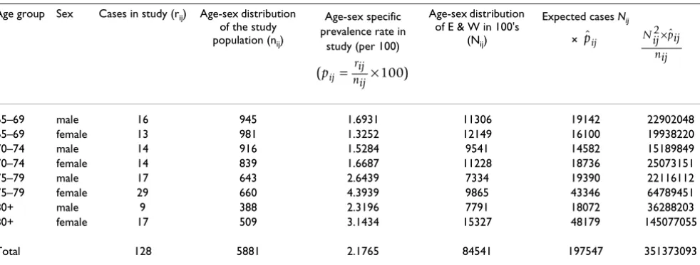
To obtain the directly standardised prevalence rate, BETS data were categorised and applied to the National tion [19]. Table 1 provides a breakdown of these popula-tions and the calculapopula-tions involved.

From [1.1] standardised

per 100 population

Using [1.3] and substituting for p_ij

Logistic method

The logistic regression analysis used disease (1 = disease present; 0 = absent) as the dependent binary variable and age (continuous), sex, and the interaction of age and sex as independent variables. Logistic regression software packages either automatically set up categorical variables as class variables, or enable the creation of dummy varia-bles (e.g. sex (1 = male, 0 = female)) with interaction terms being the corresponding products of variables.

The resultant logistic regression model for subclinical hyperthyroidism was:

Logit = - 7.2175 + 0.0461 age + 1.0337 sex - 0.0152 age*sex

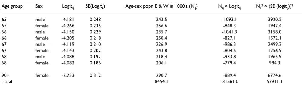
Age was found to be linearly related to the logit. The inter-action term was not significant in this model however it has been left in for illustrative purposes. Logits for all unique combinations of age and sex were then estimated from this model (e.g. a male aged 65: Logit = -7.2175 + (0.0461*65) +1.0337 - (0.0152*65) = -4.18) and weighted by the corresponding standard population size (National population estimates were available from the Office for National Statistics by gender and single year of age). This was implemented by creating a dataset contain-ing the study data plus an additional 52 'dummy' records, one for each unique combination of single year of age and sex variables but with the outcome defined as missing. The logistic regression was run with the default set up of variables and variables interactions, the resulting model being based only on the study data for which there was outcome data available (Table 2). A new output dataset containing the logits and standard error (logits) was then generated by the logistic procedure (SAS) for all observa-tions in the input dataset. The 52 'dummy' records were then extracted from this output file (Table 3) and merged with the corresponding age-sex specific standard popula-tion estimate (Table 4) to enable the following weighting calculations:

rate

Nijpij ij

N

= = =

∑ ˆ

. 197547

84541 2 337

ˆp_ij

95 1 96

2

% confidence interval standardised rate .

Nij_nijpij i

= ± jj

N ∑

95 2 337 1 96 351373093

84541 1 90 2 7 % confidence interval= . ± . =( . , . 77)

Applying [2.2] standardised logit= −31561 0= −

8454 1 3 733

.

. .

Using [2.5] standard error (standardised logit)= 57911 1 845

.

4 4 12

0 0285 .

. =

Table 1: Direct standardisation calculations for subclinical hyperthyroidism

Age group Sex Cases in study (rij) Age-sex distribution of the study population (nij)

Age-sex specific prevalence rate in

study (per 100)

Age-sex distribution of E & W in 100's

(Nij)

Expected cases Nij ×

65–69 male 16 945 1.6931 11306 19142 22902048

65–69 female 13 981 1.3252 12149 16100 19938220

70–74 male 14 916 1.5284 9541 14582 15189849

70–74 female 14 839 1.6687 11228 18736 25073151

75–79 male 17 643 2.6439 7334 19390 22116112

75–79 female 29 660 4.3939 9865 43346 64789451

80+ male 9 388 2.3196 7791 18072 36288203

80+ female 17 509 3.1434 15327 48179 145077055

Total 128 5881 2.1765 84541 197547 351373093

(p_ij rij )

nij

= ×100

ˆ

pij Nij pij

95% confidence interval for the standardised logit = standardised logit ± 1.96 standard error

(standardised logit)

-3.733 ± 1.96 (0.0285) = (-3.789, -3.677)

The standardised rate and confidence interval are then obtained using [2.3] and [2.6] respectively.

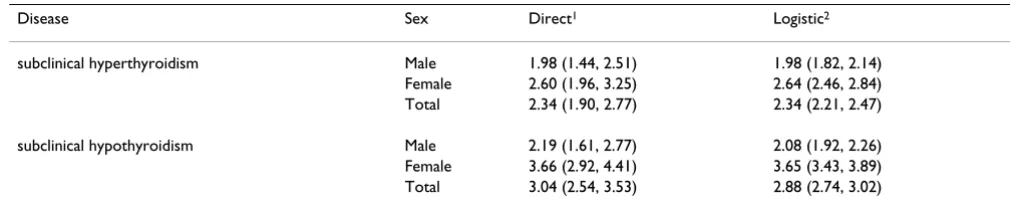
Table 5 summarises the overall and sex-specific standard-ised prevalence estimates obtained from both methods for subclinical disease. The rates were similar in magni-tude for both methods, however the confidence intervals produced by the logistic method were narrower.

Discussion

This study has illustrated the similarity of standardised rates when calculated by direct standardisation and logis-tic regression and has demonstrated the value of logislogis-tic regression in instances where individual level data are available.

Logistic regression is a practical and intuitive approach to standardisation. Most statistical packages contain regres-sion analysis procedures and the methods described in this paper are suitable for implementation in SAS and STATA (SPSS requires an additional step to obtain case-wise estimates of logit and standard error (logit) [20]).

Direct standardisation requires categorisation of the pop-ulation and the rates. If adjustment is necessary for several variables (such as age, sex and deprivation) then some cat-egories may have very low or zero rates, thus generating an imprecise estimate of the standardised rate. Once direct standardisation has been implemented, then calculation of rates is generally a routine method (requiring only the input of category specific numbers of cases) and the potential bias caused by small numbers may be missed. Logistic regression standardisation tends to fail to con-verge to a solution when the number of cases are too small, alerting the researcher to problems with the data.

The main advantage of the logistic regression method is that it allows adjustment by continuous variables in addi-tion to categorical variables and therefore has the poten-tial to lose less information than the direct method which standardised rate= −

+ − = =

exp( . ) exp( . )

. . .

3 733

1 3 733

0 024 1 024 0 02334=2 34. per 100 persons aged 65+

95 3 789

1 3 789

% exp( . )

exp( . ) , exp Confidence interval= −

+ − ⎛ ⎝

⎜ ⎞

⎠

⎟ _exp(((−._. )₎ ( . , . ) + −

⎛ ⎝

⎜ ⎞

⎠ ⎟ ⎛

⎝

⎜⎜ 1 3 6773 677 ⎞_⎠⎟⎟ = 2 21 2 47

Table 2: Logistic regression model for subclinical hyperthyroidism

Parameter DF Estimate Error Chi-Square Pr > ChiSq

Intercept 1 -7.2175 1.1495 39.4248 < .0001 age 1 0.0461 0.0154 8.9420 0.0028 sex 1 1.0337 1.1495 0.8087 0.3685 age*sex 1 -0.0152 0.0154 0.9796 0.3223

Table 3: Predicted probabilities and logits for subclinical hyperthyroidism

Obs Age Sex logit selogit varlogit

1 65 male -4.18064 0.24818 0.06159 2 65 female -4.26593 0.23466 0.05506 3 66 male -4.14982 0.22861 0.05226 4 66 female -4.20461 0.21801 0.04752 5 67 male -4.11900 0.20990 0.04405 6 67 female -4.14330 0.20189 0.04076 7 68 male -4.08818 0.19231 0.03698 8 68 female -4.08199 0.18645 0.03476

. . . .

51 90+ male -3.41019 0.40868 0.16702 52 90+ female -2.73314 0.31215 0.09744

Table 4: Logistic regression standardisation calculations for subclinical hyperthyroidism

Age group Sex Logit_ij SE(Logit_ij) Age-sex popn E & W in 1000's (N_ij) N_ij × Logit_ij N_ij2 _{× (SE (logit} ij))2

65 male -4.181 0.248 243.5 -1093.1 3920.2

65 female -4.266 0.235 256.6 -848.3 1947.4

66 male -4.150 0.229 235.7 -1041.3 3158.0

66 female -4.205 0.218 250.4 -827.1 1572.1

67 male -4.119 0.210 226.9 -986.3 2499.2

67 female -4.143 0.202 243.8 -804.5 1256.9

68 male -4.088 0.192 218.4 -933.8 1965.9

68 female -4.082 0.186 206.1 -779.4 994.3

.

90+ female -2.733 0.312 290.7 -889.4 6774.6

only allows for standardisation by categorical variables. The allowance of continuous variables also has a benefi-cial smoothing effect on the model. Logistic regression standardisation can also allow for adjustment by non-lin-ear variables and interactions between variables. The structure of the model can be extended to include random effects [21]. This may be particularly useful when allowing for clustering effects (e.g. hospitals, general practices), thereby incorporating cluster variation in the standard error of the predicted values. The logistic regression method also allows standardisation when there is missing data through the process of imputation whereas the direct method would exclude these observations from the anal-ysis [22]. In addition this method will identify the amount of variation explained by the variables and will highlight those that have a significant effect on the out-come, giving the analyst the choice to include or exclude variables [18]. Nevertheless, to avoid the problem of data dredging any potential variables should be decided on prior to analysis being performed [23].

Another possible benefit of logistic regression standardi-sation is that the method may identify the absence of sig-nificant variables and consequently demonstrate that there is no requirement or benefit from standardisation.

Conclusion

Logistic regression based standardisation is a practical alternative to the direct method. It produces more dependable estimates than the direct method when there are small numbers involved. It has greater flexibility in factor selection and allows standardisation by both con-tinuous and categorical variables. It also has the benefit of a smoothing property when including continuous varia-bles. The method allows standardisation to be performed where the direct method would give unreliable results.

Competing interests

The authors declare that they have no competing interests.

Authors' contributions

AR and RH planned the study. AR conducted the analyses and produced the first draft of the manuscript. RH pro-vided guidance on statistical analysis. All authors contrib-uted to the reviewing and editing of the manuscript. All authors read and approved the final manuscript.

Acknowledgements

We would like to thank the Birmingham Elderly Thyroid Team for allowing us access to the study data. AR was funded through the Research Support Facility, a Department of Health funded Academic Unit during the period this work was completed. Sue Wilson is funded by a National Primary Care Career Scientist Award.

References

1. Jarman B, Gault S, Alves B, et al.: Explaining differences in English hospital death rates using routinely collected data. BMJ 1999, 318:1515-20.

2. Roberts SE, Goldacre MJ: Time trends and demography of mor-tality after fractured neck of femur in an English population, 1968–98: database study. BMJ 2003, 327:771-775.

3. Department of Health. NHS performance indicators: Febru-ary 2002 [http://www.performance.doh.gov.uk/nhsperformancein dicators/2002/ha.html]

4. Lakhani A, Coles J, Eayres D, Spence C, Rachet B: Creative use of existing clinical and health outcomes data to assess NHS performance in England: Part 1–performance indicators closely linked to clinical care. BMJ 2005, 330:1426-1431. 5. Bos V, Kunst AE, Garssen J, Mackenbach JP: Socioeconomic

ine-qualities in mortality within ethnic groups in the Nether-lands, 1995–2000. J Epidemiol Community Health 2005, 59:329-335. 6. Baumert JJ, Erazo N, Ladwig K: Sex- and age-specific trends in mortality from suicide and undetermined death in Germany 1991–2002. BMC Public Health 2005, 5:61.

7. Lorant V, Kunst AE, Huisman M, Costa G, Mackenbach J: Socio-eco-nomic inequalities in suicide: a European comparative study.

Br J Psych 2005, 187:49-54.

8. Sim HG, Cheng CWS: Changing demography of prostate can-cer in asia. Eur J Cancer 2005, 41:834-845.

9. Daly LE, Bourke GJ: Interpretation and uses of medical statis-tics. Oxford, UK: Blackwell Publishing; 2000.

10. Allardyce J, Boydell J, Van Os J, et al.: Comparison of the incidence of schizophrenia in rural Dumfries and Galloway and urban Camberwell. Br J Psych 2001, 179:335-339.

11. Kendrick S, Macleod M: Adjusting outcomes for case mix: indi-rect standardisation and logistic regression. Clinical Indica-tors Support Team Working Paper. Clinical Available from Indicators Support Team Web Site. [http:// www.show.scot.nhs.uk/indicators/work/papersintro.htm].

12. Ferguson B, Gravelle H, Dusheiko M, Sutton M, Johns R: Variations in practice admission rates: the policy relevance of regres-sion standardisation. J Health Serv Res Policy 2002, 7:170-176. Table 5: Comparison of standardised rates using direct and logistic regression approaches

Disease Sex Direct1 _Logistic2

subclinical hyperthyroidism Male 1.98 (1.44, 2.51) 1.98 (1.82, 2.14) Female 2.60 (1.96, 3.25) 2.64 (2.46, 2.84) Total 2.34 (1.90, 2.77) 2.34 (2.21, 2.47)

subclinical hypothyroidism Male 2.19 (1.61, 2.77) 2.08 (1.92, 2.26) Female 3.66 (2.92, 4.41) 3.65 (3.43, 3.89) Total 3.04 (2.54, 3.53) 2.88 (2.74, 3.02)

Publish with BioMed Central and every scientist can read your work free of charge "BioMed Central will be the most significant development for disseminating the results of biomedical researc h in our lifetime."

Sir Paul Nurse, Cancer Research UK

Your research papers will be:

available free of charge to the entire biomedical community peer reviewed and published immediately upon acceptance cited in PubMed and archived on PubMed Central yours — you keep the copyright

Submit your manuscript here:

http://www.biomedcentral.com/info/publishing_adv.asp

BioMedcentral 13. Gravelle H: Measuring income related inequality in health:

standardisation and the partial concentration index. Health Econ 2003, 12:803-829.

14. Wagstaff A, Van Doorslaer E: Measuring and testing for inequity in the delivery of health care. J Hum Resour 2000, 35:716-733. 15. Dr Foster. The Hospital Guide 2006 [http://www.drfos

ter.co.uk/hospitalreport/pdfs/methodology.pdf]

16. Bottle A, Aylin P: Mortality associated with delay in operation after hip fracture: observational study. BMJ 2006, 332:947-951. 17. Wilson S, Parle JP, Roberts L, et al.: Prevalence of subclinical thy-roid dysfunction and its relation to socioeconomic depriva-tion in the elderly: a community based cross-secdepriva-tional survey. J Clin Endocrinol Metab 2006, 91(12):4809-16.

18. Hosmer DW, Lemeshow S: Applied logistic Regression 2nd edition. New York, USA: Wiley; 2000.

19. Office for National Statistics. Mid-2003 Population Esti-mates T12: Quinary age groups and sex for health areas in England and Wales; estimated resident population [http:// www.statistics.gov.uk/statbase/Product.asp?vlnk=15106]

20. Sofroniou N, Hutcheson GD: Confidence intervals for the pre-diction of logistic regression in the presence and absence of a variance-covariance matrix. Understanding Statistics 2002, 1(1):3-18.

21. Kirkwood BR, Sterne JAC: Chapter 31: Analysis of clustered data. In Essential medical statistics 2nd edition. Oxford, UK: Blackwell publishing; 2003:355-369.

22. Schafer JL, Graham JW: Missing data: our view of the state of the art. Psychological Methods 2002, 7(2):147-77.

23. Vandenbroucke JP: Statistical modelling: the old standardisa-tion problem in disguise. J Epidemiol Community Health 1989, 43:207-208.

Pre-publication history

The pre-publication history for this paper can be accessed here: