Probabilistic framework for image understanding applications using Bayesian Networks

Rochester Institute of Technology

RIT Scholar Works

Theses

Thesis/Dissertation Collections

12-1-2011

Probabilistic framework for image understanding

applications using Bayesian Networks

Mustafa Jaber

Follow this and additional works at:

http://scholarworks.rit.edu/theses

This Dissertation is brought to you for free and open access by the Thesis/Dissertation Collections at RIT Scholar Works. It has been accepted for inclusion in Theses by an authorized administrator of RIT Scholar Works. For more information, please [email protected].

Recommended Citation

Probabilistic Framework for Image Understanding

Applications Using Bayesian Networks

By

Mustafa I. Jaber

M.S. Electrical Engineering, Rochester Institute of Technology, USA, 2007

B.S. Electrical Engineering, Islamic University of Gaza, Palestine, 2003

A dissertation submitted in partial fulfillment of the

requirements for the degree of Doctor of Philosophy in the

Chester F. Carlson Center for Imaging Science,

College of Science

Rochester Institute of Technology

December 2011

Signature of the Author _______________________________

II

CHESTER F. CARLSON CENTER FOR IMAGING SCIENCE

COLLEGE OF SCIENCE

ROCHESTER INSTITUTE OF TECHNOLOGY

ROCHESTER, NEW YORK

CERTIFICATE OF APPROVAL

Ph.D. DEGREE DISSERTATION

The Ph.D. Degree Dissertation of Mustafa I. Jaber has

been examined and approved by the dissertation

committee as satisfactory for the dissertation required for

the Ph.D. degree in Imaging Science

___________________________________________________

Dr. Eli Saber,

Dissertation Advisor

___________________________________________________

Dr. Harvey Rhody

___________________________________________________

Dr. Sohail Dianat

___________________________________________________

Dr. Chance M. Glenn, Sr.

III

Dedication

IV

Acknowledgments

I would like to acknowledge and extend my heartfelt gratitude to the wonderful people who made this achievement possible. It is a pleasure to present my sincere thanks to my dissertation advisor, Dr. Eli Saber for his encouragement and guidance. I am also grateful to Dr. Harvey Rhody, Dr. Sohail Dianat, and Dr. Chance Glenn, Sr. for serving on the research committee.

Special thanks to Sue Chan, Patti Vicari, Florence Layton, and James Stefano for their help and support.

I am also very grateful to Mark Bailly and M. Sezer Erkilinc for their help and contributions in various topics of this dissertation.

Many thanks to Sreenath Rao Vantaram, Abdul Haleem Syed, and all other current and previous colleagues in the HP lab for their feedback and reviews.

Deepest gratitude to my friends especially Gregory Tsagkatakis, Prudhvi Gurram, Mohammed YousefHussien, and Yuqiong Wang. Thank you all for always being there.

Most especially, I would like to express my gratitude to my parents and family for their understanding and endless love, through the duration of my graduate study.

I am also grateful to the Center for Imaging Science and the Electronic & Microelectronic Engineering Department at the Rochester Institute of Technology for supporting this dissertation.

Finally, I am thankful to the Hewlett-Packard's Company for their generous support of this work.

Mustafa I. A. Jaber Rochester, NY

V

Probabilistic Framework for Image Understanding Applications Using

Bayesian Networks

by

Mustafa I. Jaber

Submitted to the Chester F. Carlson Center for Imaging Science in

partial fulfillment of the requirements for the Doctor of Philosophy

Degree at the Rochester Institute of Technology

Abstract

Machine learning algorithms have been successfully utilized in various systems/devices. They have the

ability to improve the usability/quality of such systems in terms of intelligent user interface, fast

performance, and more importantly, high accuracy. In this research, machine learning techniques are used

in the field of image understanding, which is a common research area between image analysis and

computer vision, to involve higher processing level of a target image to “make sense” of the scene

captured in it. A general probabilistic framework for image understanding where topics associated with (i)

collection of images to generate a comprehensive and valid database, (ii) generation of an unbiased

ground-truth for the aforesaid database, (iii) selection of classification features and elimination of the

redundant ones, and (iv) usage of such information to test a new sample set, are discussed. Two research

projects have been developed as examples of the general image understanding framework; identification

of region(s) of interest, and image segmentation evaluation. These techniques, in addition to others, are

combined in an object-oriented rendering system for printing applications. The discussion included in this

doctoral dissertation explores the means for developing such a system from an image understanding/

processing aspect.

It is worth noticing that this work does not aim to develop a printing system. It is only proposed to add

some essential features for current printing pipelines to achieve better visual quality while printing

images/photos. Hence, we assume that image regions have been successfully extracted from the printed

document. These images are used as input to the proposed object-oriented rendering algorithm where

methodologies for color image segmentation, region-of-interest identification and semantic features

extraction are employed. Probabilistic approaches based on Bayesian statistics have been utilized to

VI

Contents

1 Introduction …………..………... 1

1.1 Problem Statement and Motivations ……… 2

1.1.1 Region of Interest in Digital Images ……….……….…... 3

1.1.2 Image Segmentation Evaluation ………... 4

1.2 Research Goals ……….. 5

1.3 Intellectual Merit and Broader Impacts ………..………….. 5

1.4 Organization ………..… 6

2 Background – General Framework for Image Understanding Using Bayesian Networks .……… 8

2.1 Dataset ……….……. 9

2.1.1 Image-Set ……….…… 9

2.1.2 Ground-truth and Psychophysical Experiments ……….. 10

2.2 Image Processing Strategy and Feature Space ……… 11

2.2.1 Content- and Context-Driven Techniques in Image Understanding ………... 12

2.2.2 Feature Space and Dimensionality Reduction ……… 12

2.3 Discretization Methods ………... 14

2.4 Bayesian Networks ………. 16

2.4.1 Representation ………. 17

2.4.2 Inference ………. 18

2.4.3 Learning ……….. 19

2.5 Evaluation Tools ………. 21

2.6 Summary ………. 22

3 Bayesian Network-Based Approach for Identifying Regions of Interest in Digital Images……... 23

3.1 Background and Literature Review ……… 23

3.2 Proposed Algorithm ……… 26

3.2.1 Supervised Learning Phase ………. 28

3.2.2 Unsupervised Testing Phase ………... 37

3.3 Results ………. 39

3.4 Performance Evaluation ……….. 43

3.4.1 Comparison with work done by Pinneli and Chandler ………... 43

3.4.2 Comparison with work done by Liu et al. ………... 44

VII

4 Image Segmentation Evaluation Using Bayesian Networks ……….……….…………... 50

4.1 Background and Literature Review ……… 50

4.2 Proposed Algorithm ……….... 53

4.2.1 General-Purpose ISE Technique ………. 54

4.2.2 ROI-Specific ISE Technique ……….. 62

4.3 Results and Performance Evaluation ……….. 66

4.3.1 Performance of the Image Segmentation Evaluation Modules ………... 66

4.3.2 Using the ISE Algorithms for generating ROI Maps ……….. 69

4.4 Summary ………. 71

5 Proposed Framework for Object–Oriented Rendering in Printing Systems ………...…... 72

5.1 System Overview ……… 72

5.2 Page Layout Classification ………. 74

5.3 Image Pre-processing (Image Stitching) ………. 79

5.3.1 System Setup for Image Stitching ………... 79

5.3.2 Image Stitching Proposed Algorithm ……….. 81

5.3.3 Results from the Proposed Image Stitching Algorithm ……….. 89

5.4 Region of Interest Detection ………... 91

5.5 Image Segmentation Evaluation ….……….…………... 91

5.6 Semantic Feature Analysis (Memory Color Extraction) ………. 91

5.6.1 Proposed Memory Color Classifier ……… 92

5.6.2 Results from the Memory Color Classifier ………. 95

5.7 Summary ………. 98

6 Summary and Conclusions ………..………..…... 99

Chapter 1

Introduction

Research in vision, the most advanced of our senses, that is applied to digital images can be categorized

into three areas as described in [1] (see Figure 1.1). The first research area, digital image processing,

employs low-level features or primitive operations for noise reduction, contrast enhancement, and image

sharpening in the generated image. Notice that the input and output of an image processing system are

images. The second area of research is image analysis. It employs mid-level features to address tasks such

as segmentation (partitioning an image into regions or objects). Image analysis systems usually provides

attributes (reduced form of the data presented in the input image) that are suitable for further computer

processing and classification. That is, edge map, contours, and the identity of individual regions (objects)

are examples of such systems. The third research field is computer vision which involves higher

processing level of the image to “make sense” of the scene captured in it. Computer vision includes

algorithms from machine learning and artificial intelligence to emulate human intelligence. We identify

our research interest as image understanding, which is a common area between image analysis and

computer vision as shown in Figure 1.1.

Algorithms for image understanding are categorized according to the learning methodology to supervised

and unsupervised. In the supervised learning, training data is used to infer a model and apply that model

to test data. Example techniques include Support Vector Machine, Bayesian Networks, and Neural

Networks. It is worth noticing that the goal of the learning algorithm is to minimize the error with respect

to the given inputs (training set). However, unless the training set is comprehensive and preventative of

the original model, learning training set that well is not necessarily the best thing to do. This is a common

problem in supervised learning methodologies which is known as “over-fitting” the data and essentially

memorizing the training set rather than learning a more general classification technique. On the other

hand, in the unsupervised learning, no training data is required. Model inference and application both rely

on test data exclusively. Examples include clustering techniques and Self-organizing map in Neural

Networks. Unsupervised methods require sufficient data and iterative computations to perform well.

Figure 1.1: Systems in computational vision

System

Digital Image Processing (Low-level Feature) Image Analysis

(Mid-level Feature)

Image Understanding Computer Vision

(High-level Feature)

Input

Digital Image

Output

2 In this work, a framework for image understanding based on Bayesian Networks is introduced. A

theoretical discussion is included as well as a practical example for identifying region of interest in digital

images. Another example that aims to identify an optimal segmentation map for a target image is

proposed. Furthermore, a system for object–oriented rendering is also discussed in this dissertation. This

chapter serves as an introduction to the dissertation document. It contains sections for problem statement

and motivation, research goals, contributions to the fields of computer vision and image processing, and

lastly, the organization for the following chapters.

1.1 Problem Statement and Motivations

The goal of this research is to develop image understanding algorithms that have wide usability in image

analysis and computer vision fields. Machine learning techniques have been adopted to solve the problem

of identifying region of perceptual interest in digital images. An algorithm that utilizes BN has been

developed and evaluated using multiple image sets. Yet, another algorithm is proposed to address the

problem of selecting the optimal segmentation map that fits a given image from a set of segmentations.

The following subsections illustrate these two problems and serve as the motivation behind this research

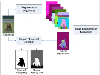
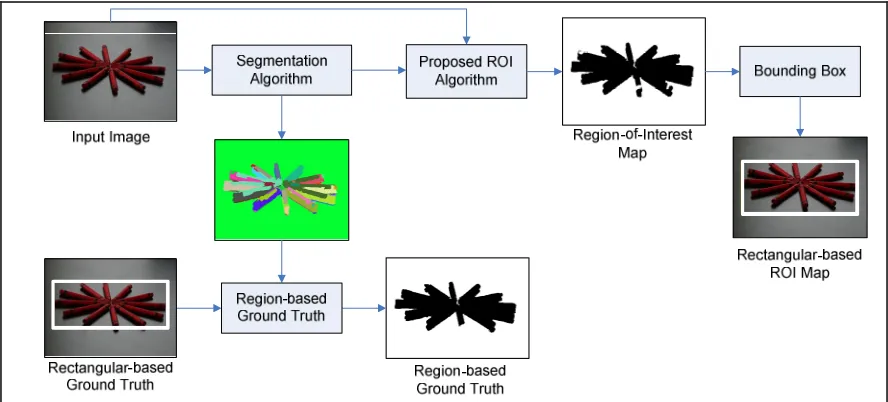
study. Figure 1.2 shows the overall system as it has modules for image segmentation, segmentation

evaluation, and region of interest detection.

3 1.1.1 Region of Interest in Digital Images

Figure 1.3 shows an example of a portrait image from the Berkeley segmentation dataset [2]. The Region

Ranking Map (RRM) for this image is also included in the figure. It is a map that quantifies the visual

significance of a particular image region in relation to other regions. In the RRM, light shades mean high

priority regions while dark shades identify background. In the example image, the face region has the

highest importance level, followed by the lady’s hair, shirt, and finally the background. In this research,

we try to simulate such visual understanding for digital images. Developing a RRM is highly subjective

because one human observer would assign the same priority level for the lady’s face and hair (less

number of significance levels) while another would pick the eyes, nose and lips at the first level of visual

significance and the skin-tone of the face at the second level and so on which would result in more levels

of perceptual importance. Note that the proposed analysis does not classify the semantic meaning of the

gray-levels in the RRM. That is, the RRM does not convey any information about the image semantic

class (skin tone, sky, grass, water, among others) of a given region. It only determines a region’s

perceptual priority. Furthermore, the RRM has multiple levels of priority. The number of these levels

(gray-shades) depends on the image content. Simpler images (one main object and smooth background)

would have few levels of visual significance while complex images may contain several of them.

(a) Color Image (b) Lighter shades signify higher visual priority

Figure 1.3: Region Ranking Map

While generating a RRM as the one given in Figure 1.2 is suitable for use in some computer vision

applications, developing a binary region-of-interest (ROI) map would add more value to other computer

vision/ image processing applications. Hence, a methodology for quantizing the RRM into two levels

(main object and background) is also proposed. Figure 1.4(b) shows an example where the bear (and the

4

(a) Color Image (b) Black shows main object and white stands for background.

Figure 1.4: Region of Interest Binary Map

1.1.2 Image Segmentation Evaluation

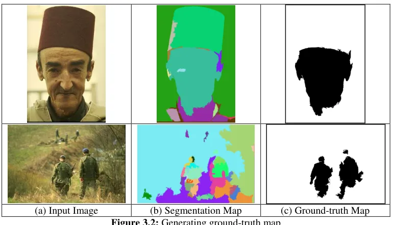
In the psychophysical experiment in [2], several observers have been asked to manually segment each

image (in a set of images) to generate meaningful maps. Their study yielded several valid segmentations

for any target image given the image content is complex “detailed” enough to be grouped at different

level while keeping the segmentation semantically meaningful. This assumption is more suitable for

natural scene imagery such as the ones used in [2]. Figure 1.5 shows a “segmentation spectrum” of a

target image which describes a few of its possible segmentation maps. The extreme over-segmentation is

to categorize each pixel to be an independent segment and thus such a map would look like an image of

random noise. On the other extreme, the ultimate under-segmented map categorizes all image pixels to

one region. If one thinks of any meaningful segmentation as a valid realization that occurs on the

segmentation spectrum, they would take place when a local minimum in the feature space is found. The

goal of this research is to develop an image understanding algorithm for ranking segmentation maps of an

arbitrary image to different levels according to their usefulness and to identify the optimal “most useful”

one. What is useful depends on the specific “target” application.

5 1.2 Research Goals

The goal of this doctoral study is to develop image understanding algorithms for identifying regions of

visual interest and image segmentation evaluation. The goals are detailed as following:

1- Develop in-depth understanding of the machine learning field while focusing on BN and utilize

such knowledge to develop image understanding algorithms.

2- Develop an image understanding algorithm for identifying region of visual interest in digital

images. This includes collecting image sets, developing ground-truth maps, running

psychophysical experiments, testing the algorithm, and evaluating its performance against

state-of-the-art techniques.

3- Develop an image understanding algorithm for image segmentation evaluation. Similar to the

second objective, this includes collecting image sets, developing ground-truth maps, running

psychophysical experiments, testing the algorithm, and evaluating its performance against

State-of-the-art techniques.

4- Utilize the algorithms developed as a part of achieving the second and third objectives to propose

a framework for object–oriented rendering in printing systems. In addition to identifying ROI and

segmentation evaluation modules, this includes modules for document analysis and raster

classification, image stitching, and memory color detection.

1.3 Intellectual Merit and Broader Impacts

The main objective of developing algorithms for image understanding is to add visual intelligence to

systems around us. Two open-problems in computer vision field have been identified; namely: region of

interest detection and image segmentation evaluation. Novel solutions are proposed to address these

issues using machine learning techniques. Furthermore, an imaging system that combines these solutions

is also proposed for real-life application. This research gains its significance from its applicability to

several imaging systems where algorithms for identifying ROI and image segmentation evaluation could

be used at a pre-processing stage for performance enhancement. Developing solutions for computer vision

problems require knowledge from several areas such as psychophysical experiment, mathematical

modeling, and machine learning. Such tools, among others, have been utilized in this research.

Experiments, proposed solutions, and results are published in conference and peer-reviewed journal

papers which will lead to further research in related fields.

The proposed solutions have direct impact of enhancing the performance of imaging systems such as

6 intermediate modules in systems for content-based image retrieval, digital libraries, and mobile imagery.

In summary, applications include but not limited to:

• Image compression [3] where visual quality of salient regions is maintained while high

compression ratio is applied to image background regions.

• Image summarization [4] and retargeting [5] where a smaller but faithful representation of the

original visual content is generated. A good “visual summary” should contain as much as possible

visual information from the input image while introducing as few as possible new visual artifacts,

that it, preserve visual coherence [6].

• Image thumbnailing [7] and cropping [8] where the ROI is cropped and down-sampled to be used

an image thumbnail in digital libraries.

• Picture collage [9] where group of images are automatically arranged on a given canvas, allowing

overlay, while maximizing their visible visual information.

• Variable data printing [10] where saliency maps ensure high quality on-demand prints while

elements such as text, graphics and images may be changed from one printed piece to the next.

• Image watermarking [11] where the system embeds watermark information to the least salient

pixels of the image.

• Assisted content creation [12] where saliency maps are used to retrieve multiple images with

similar content to have them attached to a written document.

In addition, the proposed solutions have broader impacts when used in printing system where resources’

consumption like ink (toner) is reduced while maintaining high quality prints. The proposed solutions also

would save power energy and physical memory space in case they are used in image/video compression

systems while maintaining high quality image and video signals. Furthermore, developing image

understanding algorithms would open doors for new systems such as autonomous navigation which

would turn combat vehicles into autonomous mobile platforms.

1.4 Organization

The rest of this document is organized as follows: Chapter 2 introduces a probabilistic framework for

image understanding. It has subsections on dataset collection, ground-truth generation, and image

processing strategies, feature selection, dimensionality reduction, discretization methods, Bayesian

Networks, and evaluation tools. Chapter 3 describes the proposed algorithm for identifying region of

interest in digital images. It also contains a subsection on background material and literature review on

the topic. Chapter 4 introduces the problem of image segmentation evaluation. The proposed framework

7 page layout classifier, image stitching algorithm, and memory color classifier is also included. In Chapter

6, a summary of the accomplished work is presented and recommendations for future work are also

introduced. It is worth noticing that there is no specific chapter for background and literature review

material as the author found including them in respective chapters is less confusing and ensures the

Chapter 2

Background – General Framework for Image Understanding Using

Bayesian Networks

The field of image understanding using machine learning methods has been developed by scientists’

contributions from different fields such as statistics, mathematics, psychophysics, and computer vision.

The statistical aspect of the problem deals with the collected data and whether or not it is comprehensive

enough to draw sufficient statistics. The mathematical aspect, on the other hand, studies the space

dimensionality of the data and validates the assumptions for generality. Furthermore, psychophysical

researchers’ main objective is to discover the relation between the collected data and the human response

(behavior). Therefore, the computer vision field utilizes the tools (studies) from these various divisions,

among others, to develop algorithms that would behave relationally and make decisions as a human

would do based on visual data (images and video sequences). In this chapter, we introduce a general

framework for image understanding where each section includes a step that contributes to its structure.

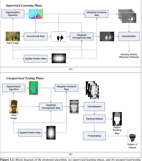
Figure 2.1 shows a block diagram of the discussed framework. Two main modules (training and test) are

shown where the training module utilizes the ground-truth data to train a classifier (based on Bayesian

Networks in our case) and the test module uses that classifier to understand the image. Both modules

share steps of feature extraction and discretization as shown in the figure. Moreover, a pre-processing step

(segmentation algorithm) is included in Figure 2.1 to indicate the necessity for such processing in some

image understanding algorithms for generality purposes.

9 This chapter is organized as follows. Methods for collecting statistically sufficient and comprehensive

data set (set of images in our case) are discussed in the first section. Methodologies for generating

ground-truth data (by human observers) for the collected image-set are also discussed. In section two,

content- and context-driven techniques in image understanding have been introduced in addition to

discussions on feature selection, feature space, and dimensionality reduction. The third section introduces

the discretization problem which converts the continuous space that the proposed features lives in to a

low-computational discrete form. Furthermore, the Bayesian Network (BN) theory is introduced in the

fourth section where topics like optimum network structure, parameter learning, and inference have been

discussed. Next, the fifth section which is entitled “Evaluation Tools”, discusses several methodologies

for evaluating image-understanding algorithms. Finally, a summary of this chapter is presented in the last

section.

2.1 Dataset

The behavior of machine learning based algorithms is highly correlated to the datasets utilized in its

training and testing. Having a comprehensive and unbiased dataset is essential; furthermore, having a

valid ground-truth for that dataset is extremely critical. In this section, questions about the dataset itself

such as how to collect a dataset, and how to validate that it is comprehensive and statistically sufficient

have been addressed. Furthermore, issues related to ground-truth, in terms for building a ground-truth and

validating it, are also discussed.

2.1.1 Image-Set

In image understanding applications, the test target is usually an image, a set of images, or a video

sequence. However, additional metadata, usually stored in an exchangeable image file format, such as

aperture, exposure time, focal length, date and time taken, and location could be used to help in the

understanding process. Geocoded Photography is an example application that associates the image with

its geographical location at the time of capture. In this work, our main objective is to develop a

framework to process images (without any additional metadata) to gather a better understanding of their

content.

Having access to a numerous number of digital images has become relatively easy with the development

of web search engines and the wide spread use of digital cameras (among other resources). Collecting any

number of such images into a set would generate an image-set (issues related to intellectual property and

ownership are not discussed here but must be considered). However, using such an image-set to develop

10 and comprehensive image-set? Does is it have an unbiased ground-truth data (map) associated with each

image? An attempt to answer the first question is included in the following paragraphs. Furthermore, the

issues related to the ground-truth data are significant and thus have been addressed separately in the

following subsection.

Assume that we consider an image understanding system for identifying the main region of visual interest

in a target digital image as an example application. Ideally such system should identify the main

Region-of-Interest (ROI) in any digital image under any capturing and viewing circumstances. However, an ideal

system like this does not exist yet. To this effect, limiting the scope of the algorithm would enhance its

overall performance (maximizing the hits and minimizing the false alarms, for example). Limiting its

scope means defining some assumptions about the type of images used to build and test the algorithm

(vacation, real-life and natural images, medical images, hyperspectral and other remote sensing images, or

infrared images). This specific usage of ROI algorithm would increase its accuracy to acceptable levels.

In other words, one can compromise the completeness of the system (works only on one type of images)

for improved performance. On the other hand, an acceptable framework (an image-set used to train and

test the system) for identifying a ROI in specific type of images should be comprehensive, that is, it

should work fairly in any given image from that type. Comprehensive image-sets should include a large

number of images gathered from different imaging devices under different circumstances. This should

cover variations in images content and context. Finally, another important feature that one should

consider when using an image set is its ability to draw sufficient statistics, that is, no other statistic which

can be calculated from the same sample provides any additional information as to the value of the

estimated parameter.

2.1.2 Ground-truth and Psychophysical Experiments

Having a valid and unbiased human-generated data associated with the image-set is critical to develop

unbiased image understanding algorithms. The ground-truth is any data that could be measured or

generated by human in order to train and validate the performance of image understanding algorithms.

For example, estimating the physical dimension (width and height) of an object from its images could be

compared to the hand-labeled data which is the physical dimensions of the object measured (using a

measuring tape, for example) in the real word. The ground-truth data could be an objective quantity that

could be physically measured (such as height, weight, or distance) or it could be a subjective

understanding that needs to be estimated. Psychophysical experiments and observer studies are usually

used to generate the later type of ground-truth data as the case in identifying the region of visual interest

11 Psychophysical experiments in image understanding field investigate the relationship between physical

stimulus which is usually an image (printed or shown digitally on a monitor) and its effects on the human

observer. The experiment could include eye-tracking devices [13] or could be simply a set of questions

that the subject has to answer [14]. Several factors should be considered when developing a

psychophysical experiment for image understanding purposes [15]. First, the main goal of the experiment

should be clear and all the assumptions should be carefully studied. It is the responsibility of the

researchers who conduct the study to explain the instructions (would be limited to written instruction

without any personal contact) to the human subjects. A pilot study is always helpful to make sure that the

instructions are clear and the experiment is well designed to achieve its objectives. The second factor is

the stimuli or the set of images selected for the experiment. The behavior of the human observers could be

affected (distracted) by the number of the test images used in the experiment, the order of showing them,

or the illumination of the surrounding environment. The third factor essential for having a successful

psychophysical experiment, is the human observers (having enough number of observers is also critical).

Their experience and expectations could bias the experiment. The observers age, gender, education,

ethnic, and background could affect their judgment as well. Another thing should be considered is that the

observers should have normal vision (or corrected to normal) with respect to color and visual acuity in

image understanding experiments. The fourth factor is the environment for conducting the experiment. It

is preferable to have fixed setup that is clean of any distractions. Furthermore, items such as lighting

conditions, eye adaptation time, viewing distance, and angle of view should be controlled in the

environment setup. The overall time that any human observer has to run the experiment or to view any

particular stimuli should be considered while developing the study. The final step utilizes a scientific

method to study the collected data from the human observers and draw the experimental findings.

Additional step, which is recommended to be included while developing observer studies, is the

validation of the experimental design using different setups and observers to ensure consistency in the

results achieved.

2.2 Image Processing Strategy and Feature Space

An overview of the processing strategies that have been utilized for image understanding in the literature

is introduced in this subsection. These methods could be limited to the visual data found in the image as

in the case of content-driven techniques or could be extended to include more contextual information as in

context-driven methods. A further expansion on the content-driven techniques has been included to

12 2.2.1 Content- and Context-Driven Techniques in Image Understanding

Content-based image understanding uses visual information found in the image (or in other words, the

value of pixel count) to extract the features used in the system. These features could be purely

pixel-based, regional information (regions are developed using image segmentation algorithms) or they could

be semantic concepts (discussed later in this section). On the other hand, the context-driven algorithms

utilized information found in the image-file header to help in the understanding process [16]. Context

information is written to the photos by most consumer digital cameras and it varies from camera to

camera. However, most cameras at least provide information like timestamp, ISO, aperture, exposure, and

if a flash was used. Some cameras also provide the focal length, the orientation and even location

information such as a GPS position [17]. Furthermore, hyped combinations of both methods are also

found in the literature.

The focus of this work is to develop image-understanding algorithms based on the visual content of a

target the image. To this effect, features such as histogram generation, edge detection, similarity analysis,

and face detection are extracted from the image. The type of features used in the content-based image

analysis could further separate them into two different categories. The first one utilizes low-level vision

features to draw an understanding of the image content and to describe its content such as skin, sky,

people, and buildings, among others. This type of analysis is known as the bottom-up approach and it

uses spatial and spectral features. The features are used to process all image pixels and the result is then

used to describe the image content. On the other hand, the top-down approach is a more goal-oriented

process where a hypothesis about the image content is proposed and high-level (semantic concepts)

features are used to test that hypothesis. The top-down approach utilizes image classifiers (indoor versus

outdoor scene) and semantic detectors (such as skin detection) as features.

2.2.2 Feature Space and Dimensionality Reduction

Feature is synonymous of input variable or attribute. It represents the image content in a conceptual space

rather than its color and spatial coordinates. Finding a good data representation is very domain specific

and related to available measurements [18]. In image processing field, attribute can be low-level vision

features or high-level features that represent semantic objects in the scene. In digital video signals,

features can be extended to include the temporal dimension. Feature extraction is a challenging problem

because identifying relevant features leads to better, faster, and easier to understand algorithm.

In general, feature extraction includes two major steps, namely, feature construction and feature selection.

13 compatible in terms of scale and values range. On the other hand, feature selection is primarily performed

to select relevant and informative features. It may also include other objectives like data reduction,

performance improvement, and data understanding. A critical aspect of feature selection is to properly

assess the quality of the features selected. Methods from classical statistics and machine learning could be

used to achieve this goal, in particular, hypothesis testing and cross-validation [18].

The processing level in image understanding algorithm is determined by the objective (desired outcome)

of the system, be it pixel, segment, image, or a set of images. In a pixel-based methodology, a classifier is

employed to determine its semantic class. Secondly, a pre-processing module for image segmentation

could be utilized to classify image pixels to different homogeneous regions. Consequently the

understanding technique is carried out at the segment-level (based on the generated segmentation map).

Thirdly, the desired outcome could be to classify a scene captured in the image as either indoor or outdoor

scenery, for example, where the processing level considers the entire target image. Finally, an ultimate

image understanding process could aim to retrieve a set of images from an image library which are

similar to a given test image as the case of contain-based image retrieval [19] and image libraries. For any

level of processing, a set of features have to be selected to build a classifier tool that would help in

making decisions for understanding purposes. The obtained features represent the image content in a

conceptual space rather than its color and spatial coordinates. The feature space is an abstract space where

each pattern sample (be it pixel, segment, image, or a set of images) is represented as a point in

n-dimensional space. Its dimension is determined by the number of features used to describe the patterns

where similar samples are grouped together.

However, one should be careful when selecting image features to avoid data redundancy, otherwise, a

further analysis step of feature extraction, a process of reducing the number of random variables under

consideration, would be required. When a feature selection stage is followed by a feature extraction step,

the entire process is known as dimensionality reduction. Reducing the dimensionality of the feature space

helps improve the performance of learning models by: 1) alleviating the effect of the

curse-of-dimensionality, 2) enhancing generalization capability, 3) providing faster and more cost-effective

learning procedure, and 4) providing a better understanding of the underlying process that generates the

data [20]. The two most widely used linear dimensionality reduction methods are Principal Component

Analysis (PCA) and Factor Analysis, both of which are based on second-order statistics. For normal

variables (with zero mean), the covariance matrix contains all information about the data. Second-order

methods are relatively simple to implement, as they require classical matrix manipulations. However,

14 dimensionality reduction methods, using information not contained in the covariance matrix, are more

appropriate such as projection pursuit which is a linear higher-order method. Independent component

analysis is another higher-order linear method. Non-linear principal component analysis can be

considered as a special case of independent component analysis. It uses non-linear objective functions to

determine the optimal weights, but the resulting components are still linear combinations of the original

variables. Random projections method is another dimension reduction technique. More details about these

dimension reduction techniques could be found in the survey by Guyon and Elisseeff [20].

2.3 Discretization Methods

Given that an attribute is either categorical or numerical where values of a categorical attribute are

discrete and values of a numeric attribute are either discrete or continuous, one can define discretization

as the conversion of a numeric attribute to a categorical one [21]. Note that this is a valid definition

irrespective of whether that numeric attribute is discrete or continuous because a categorical attribute

often takes a small number of values. Even for discrete attributes that have a finite but large number of

values, as there will be very few training instances for any one value, it is often desirable to aggregate a

range of values into a single value utilizing a discretization module. The terms categorical or numeric are

usually used to address the type of the attribute in this research area.

Discretizing numeric attributes is recommended at a pre-processing stage prior to the learning process. It

helps fitting the data with better models and it decreases the computational complexity. Unfortunately, the

number of ways to discretize a numeric attribute is infinite. Discretization is a potentially time-consuming

bottleneck, since the number of possible discretizations is exponential in the number of interval in the

domain [22]. The objective of the ideal discretization process is to minimize the number of cut-points that

partition the range of numeric attribute into a small number of coherent classes. However, in reality, a

compromise must be found between information quality (homogeneous intervals) and statistical quality

(sufficient sample size in every interval to ensure generalization). A typical discretization process broadly

consists of four steps [22]: (1) sorting the continuous values of the feature to be discretized, (2) evaluating

a cut-point for splitting or adjacent intervals for merging, (3) according to some criterion, splitting or

merging intervals of continuous value, and (4) finally enforcing termination criteria at some point.

Table 2.1: Categorization of discretization methods

Discretization

Metric 1 Metric 2 Metric 3 Metric 4 Metric 5

15 Generally, discretization methods can be categorized using different metrics as shown in Table 2.1:

(1) Supervised versus Unsupervised: A distinction can be made dependent on whether the method takes

class information into account to find proper intervals or not. Discretization methods that do not make

use of class membership information are referred to as unsupervised methods (examples include

methods, such as equal width interval binning and equal frequency binning). In contrast,

discretization methods that use class labels for carrying out discretization are referred to as supervised

methods.

(2) Direct versus Incremental: Direct methods divide the range of k intervals simultaneously (i.e.,

equal-width), needing an additional input from the user to determine the number of intervals. Incremental

methods begin with a simple discretization methodology and pass through an improvement process,

needing an additional criterion to know when to stop discretizing.

(3) Global versus Local: Global discretization handles each numeric attribute as a pre-processing step,

that is, before induction of a classifier whereas local methods carry out discretization on-the-fly

(during induction). Empirical results have indicated that global discretization methods often produced

superior results compared to local methods since the former use the entire value domain of a numeric

attribute for discretization, whereas local methods produce intervals that are applied to sub-partitions

of the instance space.

(4) Static versus Dynamic: The distinction between static and dynamic depends on whether the method

takes feature interactions into account. Static methods, such as binning and entropy-based

partitioning, determine the number of partitions for each attribute independent of the other features. In

contrast, dynamic methods conduct a search through the space of possible k partitions for all features

simultaneously, thereby capturing interdependencies in feature discretization.

(5) Top-down versus Bottom-up: Top-down methods consider one big interval containing all known

values of a feature and then partition this interval into smaller and smaller subintervals until a certain

stopping criterion (for example Minimum Description Length) or optimal number of intervals is

achieved. In contrast, bottom-up methods initially consider a number of intervals, determined by the

set of boundary points, to combine these intervals during execution until a certain stopping criterion,

such as a Chi-square (χ2) threshold, or optimal number of intervals is achieved.

As an example, three discretization methods are discussed here, namely: equal width interval binning,

16 determines the minimum and maximum values of the discretized attribute and then divides the range into

a user-defined number of equal width discrete intervals. The equal-frequency algorithm determines the

minimum and maximum values of the discretized attribute, sorts all values in ascending order, and

divides the range into a user-defined number of intervals so that every interval contains the same number

of sorted values. The weakness of the equal-width method is that in cases where the outcome observations

are not distributed evenly, a large amount of important information can be lost after the discretization

process. For equal-frequency, many occurrences of a continuous value could cause the occurrences to be

assigned into different bins. One improvement that can be employed is that after continuous values are

assigned into bins, boundaries of every pair of neighboring bins are adjusted so that all duplicate values

are assigned to a single bin. These methods are dominated by sorting and hence, their complexities are of

order O(n log n).

Both equal-width and equal-frequency discretization algorithms potentially suffer much attribute

information loss since number of intervals is determined without reference to the properties of the training

data. Wrapper based methods overcome this drawback by refining the discretization of the continuous

explanatory attributes by taking feedback from an induction algorithm. Error-based methods evaluate

candidate cut points against an error function and explore a search space of boundary points to minimize

the sum of False Positive (FP) and False Negative (FN) errors on the training set. In other words, given a

fixed number of intervals, error-based discretization aims at finding the best discretization that minimizes

the total number of errors (FP and FN) made by grouping together particular continuous values into an

interval. This methodology is mainly used in the feature selection field. In our research, we used the

wrapper approach to find the optimum number of intervals in an equal-frequency discretization

framework.

2.4 Bayesian Networks

A Bayesian Network (BN) is a directed graphical model for probabilistic relationships among a set of

variables [23]. Graphical models represent the relation between probability theory and graph theory where

a complex system could be built by combining simpler components. Probability theory provides the glue

wherein the parts are combined, ensuring that the system as a whole is consistent, and providing ways to

interface models to data. Furthermore, graph theory provides both an intuitively appealing interface by

which humans can model highly-interacting sets of variables as well as a data structure that lends itself

naturally to the design of efficient general-purpose algorithms [24]. Graphical models have been used to

study classical multivariate probabilistic systems in the fields of statistics, systems engineering,

17 graphical models, belief networks, generative models, and causal models in artificial intelligence and

machine learning communities.

In this section, representation of a BN will be discussed. It aims to show how a graphical model can

compactly represent a joint probability distribution. Second, the inference process in a BN is introduced.

It discusses how to efficiently gather states of a hidden node (variable) in a system, given partial and

possibly noisy observations. Next, a subsection on learning a BN is included where the model’s

parameters and structure are estimated.

2.4.1 Representation

Bayesian networks are graphs in which nodes represent random variables (one node per variable), and

nodes are connected to other nodes using arcs (arrows). The lack of possible arc/connection represents a

conditional independence assumption. For example, if an arrow starts at X and ends into Y, X is parent of

Y and thus X has a direct influence on Y and can be informally interpreted as indicating that X “causes" Y

[24]. Note that any point can have no parent, one parent, or multiple parents; and the same syntax applies

to the child nodes (Y is a child node in the pervious analysis). Furthermore, any node Yi has a conditional

probability distribution given its parents, P(Yi|Parents(Yi)). In the simplest case, if all nodes in the BN are

discrete (categorical) random variables, and further, that the conditional distributions are multinomials,

the conditional probability distributions could be presented as Conditional Probability Tables (CPT)

which are simple to represent, learn and use for inference [24]. Finally, BNs are Directed Acyclic Graphs

(DAG) which means they do not have any directed cycles. Figure 2.2 shows a topology example of a

network that encodes conditional independence assertions where Weather is independent of the other

variables but Toothache and Catch are conditionally independent given Cavity [25]. Note that a DAG

model which includes decision and utility nodes, as well as chance nodes, is known as an influence

(decision) diagram, and can be used for optimal decision making [24].

Figure 2.2: Bayesian network topology.

In summary, a Bayesian network for a set of variables X = {X1, … , Xn} consists of (1) a network

structure S (or a DAG) that encodes a set of conditional independence assertions about variables in X, and

18 define the joint probability distribution for X. Note that the nodes in S are in a one-to-one correspondence

with the variables X. In particular, given structure S, the joint probability distribution for X is given by:

∏

i Parents X

X p p 1 )) ( | ( ) X

( (2.1)

Local probability distributions P are the distributions corresponding to the terms in the product of

Equation 2.1. Consequently, the pair (S, P) encodes the joint distribution P(X) [23]. Note that the

probabilities encoded by a Bayesian network may be Bayesian or physical [23]. The probabilities are

Bayesian when the BN is built from prior knowledge; however, these probabilities are physical (and their

values may be uncertain) when the BN is learned from data as shown in the subsequent sections.

2.4.2 Inference

Inference implies estimating the values of hidden nodes, given the values of the observed nodes. It could

be in the form of a diagnosis, or bottom-up reasoning when we observe the “leaves” of a generative

model, and try to infer the values of the hidden causes. On the other hand, if we observe the “roots” of a

generative model, and try to predict the effects, this is called prediction, or top-down reasoning. BNs can

be used for both of these tasks [24]. The inference process is usually used to determine various

probabilities of interest from the model such as p(X|y). This is given that we have constructed a Bayesian

network from prior knowledge, data, or a combination,

∑

=

(

,

,

)

)

|

(

X

y

p

X

y

k

p

α

where X represents a set of hidden nodes that we are interested in estimating, y is the observed evidence, k

is the set of irrelevant hidden variables, and α is a scaling factor. The posterior probability in Equation 2.2

can be computed using Bayes' rule. Bayes' rule states that:

) ( ) ( ) | ( ) | ( y p X p X y p y X

p = (2.3)

or in words, this formula becomes

evidence prior x likelihood l conditiona

posterior= (2.4)

There are two kinds of inference: exact and approximate. Exact inference can be found by variable

elimination or message passing methodologies while approximate inference can be estimated by

19 Exact Inference

Exact inference is only possible in a very limited set of cases, mostly when all hidden nodes are discrete,

or when all nodes (hidden and observed) have Gaussian distributions. Exact inference could be done by a

variable elimination method or by message passing. The chain-rule decomposition (Equation 2.5) of the

joint probability is utilized to carry out summations right-to-left, storing intermediate results to avoid

recompilation. This essentially would “push sums inside products” to marginalize out the irrelevant

hidden nodes efficiently [25],[24]. The chain rule of probability is given by:

)... , | ( ) | ( ) ( ) X

( p X₁ p X₂ X₁ p X₃ X₁ X₂

p = (2.5)

or in its general form [23]:

) ,..., , | ( ) X

( _{1 2 1}

1

− =

∏

= i i

n i X X X X p

p (2.6)

In message passing algorithm, the general inference process is defined in terms of message passing on a

tree (junction tree). The messages may be passed in parallel or sequentially. Message passing method is

efficient for computing all marginals simultaneously which is necessary for learning [24].

One drawback of exact inference algorithms is that their running time is exponential in the size of the

largest cluster (assuming all hidden nodes are discrete); this size is called the induced width of the graph,

and minimizing it is NP-hard (non-deterministic polynomial-time hard). Furthermore, exact inference is

hard to estimate if some of the nodes represent continuous random variables (even in graphs with low

induced width). That is, implementing the integrals associated with the Bayes' rule cannot be performed

in closed form. Therefore, it is necessary to use approximate inference [24].

Approximate Inference

The basic idea of approximate inference is to draw a number of samples from a sampling distribution and

compute an approximate posterior probability. We need to show that the approximate posterior

probability converges to the true probability. Sampling (Monte Carlo) method, Variational method, and

belief propagation technique are popular approximate inference examples. More information about these

algorithms is found in [24] and [25].

2.4.3 Learning

The term “Learning” in a BN context may refer to the process of estimating the optimal graph topology

(network structure) that represents the causal relationships between parameters in a given dataset, the

process of estimating the joint probability distribution over a set of random variables (network

20 relationships are usually used to help in solving the learning problem. Learning the BN structure is

considered a harder problem than learning the BN parameters. Moreover, another obstacle arises in

situations of partial observability when nodes are hidden or when data is missing. In general, four BN

learning cases are often considered, to which different learning methods are proposed, as seen in Table

2.2 [24].

Table 2.2: Learning categories in a BN

Case BN Model Structure Variable Observability Proposed Learning Method

1 Known Full Maximum-likelihood estimation 2 Known Partial Expectation Maximization, Markov chain Monte

Carlo (MCMC) 3 Unknown Full Search through model space 4 Unknown Partial Expectation Maximization + Search through

model space

The first case is the simplest case where the goal of learning is to find the values of the BN parameters (in

terms of CPT) that maximize the log-likelihood of the training dataset. For example, if we assume that

this dataset contains m cases (that are often assumed to be independent). Given training dataset Σ = {x1,

…, xm}, where xl = (xl1,…, xln) T

, and the parameter set θ = (θ1,…, θn) T

, where θi is the vector of

parameters for the conditional distribution of variable Xi (represented by one node in the graph), the

log-likelihood of the training dataset is a sum of terms, one for each node [26]:

) , | ( log )

| (

log _{li i i}

m n

x P

L Θ ∑ =

∑∑

π

θ

where the contribution of each node to the log-likelihood can be maximized independently. Note that π is

the set of parents of Xi.

Furthermore, cases 2, 3, and 4 in Table 2.2 are computationally intractable in general. In case 2 where the

BN structure is known and the parameters are partially observed, Expectation Maximization (EM)

algorithm could be used to find a locally optimal maximum-likelihood estimate of the parameters [23].

An alternative approach is to use Markov Chain Monte Carlo (MCMC) to estimate the parameters of the

BN model. In the third case where the parameters are fully available but the structure is unknown, the

goal is to learn the optimal DAG that best explains the data. Note that the number of DAGs on N

variables is super-exponential in N (NP-hard problem). Some assumptions could be utilized to simplify

the problem and thus to limit the search space. One approach is to assume that the variables are

conditionally independent given a class, which is represented by a single common parent node to all the

variable nodes. This structure corresponds to the naive BN, which surprisingly is found to provide

21 to determine the order of the nodes as in K2 algorithm [27]. The last case is the hardest where one has to

marginalize out the hidden nodes as well as the parameters. Since this is usually intractable, it is common

to use an asymptotic approximation to the posterior called the Minimum Description Length (MDL)

approach where a trade-off between the likelihood term and a penalty term associated with the model

complexity is utilized. An alternative approach based on EM algorithm could be used as well [23] [25].

Figure 2.3: Categorization of evaluation methods

2.5 Evaluation Tools

The outcome of an image-understanding framework can be well-defined as the case in object recognition

(e.g. car, house, animal, airplane, etc.) or ill-defined as the case of image segmentation and

region-of-interest identification. Evaluating algorithms from the former type is easier to perform using subjective

tools; however, assessing algorithms based on ill-defined problems is not an easy task. An interesting

hierarchy of image-segmentation-evaluation methods is found in [28]; however, the hierarchy can be

generalized to any image understanding algorithm. The evaluation methods are fundamentally very

different, and can be partitioned based on four distinct methodologies as shown in Figure 2.3:

(1) Subjective versus Objective: This category indicates the enrollment of a human observer in the

subjective evaluation by judging an outcome image or by any other means. A scientific subjective

evaluation process could utilize a number of observers in a psychophysical experiment framework

(discussed in Section 2.1.2). On the other hand, an objective methodology uses measured features and

calculated metric for evaluation. Subjective evaluation technique could be biased, very tedious and

time-consuming process. Furthermore, such methods cannot be used in a real-time system.

(2) System-level versus Direct Evaluation: Both techniques are objective evaluation methods. The

system-level process indicates that the image-segmentation module serves as one (or multiple)

component of a larger system, and the evaluation is carried on all parts of the system. This could be

when a segmentation algorithm is used at a pre-processing stage in an imaging system, and the

Subjective

Objective Evaluation

Methods System-level

Direct

Analytical

Empirical

Unsupervised

22 evaluation process aims to evaluate the segmentation maps generated. Unfortunately, this evaluation

method is indirect. On the other hand, the direct evaluation is performed when the

image-understanding system is independent.

(3) Analytical versus Empirical Methods: Both methods belong to the direct objective evaluation process.

Analytical evaluation means the method itself has been validated while the empirical method

indicates that the results generated by the understanding algorithm are being examined. In an

analytical process, the algorithms are evaluated based on certain properties such as processing

strategy (parallel, sequential, iterative, or mixed), processing complexity, and resource efficiency.

These properties are generally independent of the quality of an algorithm’s outcome, so analytical

methods are not considered effective at characterizing the image understanding performance.

(4) Unsupervised versus Supervised Methods: Both methods are empirical, direct, and objective

evaluation methods. They are divided on whether the method requires a ground-truth reference image

or not. Supervised evaluation methods, also known as relative evaluation methods or empirical

discrepancy methods [28], requires a ground-truth map (gold standard) to compare the algorithm’s

result against. The degree of similarity between the human and machine generated images determines

the quality of the image understanding technique. However, the process of generating a reference

image is a difficult, highly subjective, and time-consuming task. On the other hand, unsupervised

evaluation methods, also known as stand-alone evaluation methods or empirical goodness methods

[28] do not require a reference image, but instead evaluate an image understanding outcome based on

how well it matches a broad set of characteristics as desired by humans.

2.6 Summary

An approach of image understanding has been introduced in this chapter where essential concepts/steps

for building a computer vision system are discussed. The framework uses machine learning technique

where the system is trained and evaluated using collected data in the form of ground-truth maps. Methods

for feature selection, dimensionality reduction, and discretization methods are discussed. Furthermore,

Bayesian Networks has been introduced as a probabilistic framework that uses a dataset to learn its

structure and to further use that structure in evaluating a test target. Evaluation techniques are also

introduced. Understanding each section of this chapter is essential for building a framework for image

understanding. In the following chapters, two computer vision problems will be introduced and

corresponding solution will be proposed utilizing the general image understanding framework discussed

Chapter 3

Bayesian Network-Based Approach for Identifying Regions of

Interest in Digital Images

In this chapter, an image understanding algorithm for identifying and ranking regions of perceptually

relevant content in digital images is proposed. Global features that characterize relations between image

regions are fused in a probabilistic framework to generate a Region Ranking Map (RRM) of an arbitrary

image. Features are introduced as maps for spatial position, weighted similarity, and weighted

homogeneity for image regions. Further analysis of the RRM, based on the Receiver Operating

Characteristic (ROC) curve, has been utilized to generate a binary map that signifies Region-of-Interest

(ROI) in the test image. The algorithm includes modules for image segmentation, feature extraction, and

probabilistic reasoning. It differs from prior art by using machine learning techniques to discover the

optimum Bayesian Network structure and probabilistic inference. It also eliminates the necessity for

semantic understanding at intermediate stages. Experimental results indicate an accuracy rate of ~80% on

a set of ~20,000 color images which are publicly available and compare favorably with the state-of-the-art

techniques.

3.1 Background and Literature Review

The primary objective in developing algorithms for identifying regions of visual interest in digital images

is to improve the sophistication of subsequent image processing applications. Different terminologies for

Regions-of-Interest (ROI) such as Main Subject Detection (MSD), Object-of-Interest (OOI), Importance

Map (IM) and Region Ranking Map (RRM) are found to be used interchangeably in the literature. These

algorithms can be utilized by printing companies, for example, to develop smart document rendering

where different regions could be rendered according to their visual significance and content. Furthermore,

ROI algorithms can be employed at a pre-processing stage in adaptive compression and coding systems

where the compression quality of perceptually important regions should be higher than other regions

(background) of the image [29] [30]. Other applications include content-based image retrieval [19] [31]

[32], image indexing [33], automatic image annotation [34], region classification [35], medical imaging

[36], and digital photo cropping [37].

Several techniques have been proposed in the literature to identify ROI, including human Visual

Attention (VA) modeling and saliency maps generation. Algorithms for extracting main objects in low

Depth-of-Field (DOF) images were proposed in [38], [39], and [40]. Low DOF imaging primarily focuses

24 human VA to the object in focus [38], [39]. Methods for detecting ROI in low DOF images employ tools

such as frequency-band filters and wavelet analysis. However, their performance is affected when

background (blurred) regions have high-frequency texture such as grass in outdoor images in which case

background regions could be classified as parts of the OOI. Furthermore, such algorithms ignore the

significance of other low-level vision features such as color and spatial position. In [38], wavelet

transform and statistical analysis have been used to perform context-dependent classification of individual

blocks of the image to background and foreground. A set of 100 low DOF images has been used to

evaluate the algorithm’s performance. The algorithm has been developed with and 3D microscopic image

analysis and biomedical image segmentation in mind. In general, algorithms for automatic object

segmentation in images with low DOF apply thresholding methods in feature space to separate focused

objects and defocused background. T