This is a repository copy of
Positivity-preserving scheme for two-dimensional
advection-diffusion equations including mixed derivatives
.
White Rose Research Online URL for this paper:
http://eprints.whiterose.ac.uk/128656/
Version: Submitted Version
Article:
Du Toit, Erasmus J., O'Brien, Martin R. and Vann, Roderick G L
orcid.org/0000-0002-3105-2546 (2018) Positivity-preserving scheme for two-dimensional
advection-diffusion equations including mixed derivatives. Computer Physics
Communications. ISSN 0010-4655
https://doi.org/10.1016/j.cpc.2018.03.004
[email protected] https://eprints.whiterose.ac.uk/ Reuse
Items deposited in White Rose Research Online are protected by copyright, with all rights reserved unless indicated otherwise. They may be downloaded and/or printed for private study, or other acts as permitted by national copyright laws. The publisher or other rights holders may allow further reproduction and re-use of the full text version. This is indicated by the licence information on the White Rose Research Online record for the item.
Takedown
If you consider content in White Rose Research Online to be in breach of UK law, please notify us by
Positivity-preserving scheme for two-dimensional advection-diffusion equations
including mixed derivatives
E.J. du Toita,b,∗, M.R. O’Brienb, R.G.L. Vanna
a
York Plasma Institute, Department of Physics, University of York, York, YO10 5DD, UK b
Culham Centre for Fusion Energy, Abingdon, OX14 3DB, UK
Abstract
In this work, we propose a positivity-preserving scheme for solving two-dimensional advection-diffusion equations including mixed derivative terms, in order to improve the accuracy of lower-order methods. The solution to these equations, in the absence of mixed derivatives, has been studied in detail, while positivity-preserving solutions to mixed derivative terms have received much less attention. A two-dimensional diffusion equation, for which the analytical solution is known, is solved numerically to show the applicability of the scheme. It is further applied to the Fokker-Planck collision operator in two-dimensional cylindrical coordinates under the assumption of local thermal equilibrium. For a thermal equilibration problem, it is shown that the scheme conserves particle number and energy, while the preservation of positivity is ensured and the steady-state solution is the Maxwellian distribution. Keywords: Advection-diffusion, Fokker-Planck equation, low-order positivity-preserving scheme
1. Introduction
Two dimensional advection-diffusion equations have widespread applications in physics, engineering and finance, and can generally be written as
ut=Auxx+Buxy+Cuyy+Dux+Euy+F u (1)
whereu=u(x, y, t). As these equations are often too difficult to solve analytically, numerical solutions are required. ForF = 0, these equations can be written in a two-dimensional advection-diffusion form,
∂u ∂t =∇ ·
−~au+ ˆk· ∇u (2)
where u = u(x, y, t) is advected by the 2D vector ~a(x, y, t) and diffused by the tensor ˆk(x, y, t). A particular application of two-dimensional advection-diffusion equations is the Fokker-Planck collision operator, which can typically be written in the form (2) and has a wide range of applications in plasmas in the laboratory (e.g. magnetic and inertial thermonuclear fusion), space (e.g. Earth’s magnetosphere), and astrophysics (e.g. solar coronal mass ejections) [1].
If the initial conditionu(x, y,0)≥0 holds for all (x, y), then the solution must always be positive, i.e. u(x, y, t)≥ 0 for all (x, y, t). Moreover, a good numerical method has to preserve the monotonicity of the initial condition. The conservation of such properties poses a particular challenge if a change of coordinates, adopted to eliminate the mixed derivative terms uxy throughout (x, y) space, is not possible.
Positivity-preserving schemes to two-dimensional advection-diffusion equations, in the absence of mixed deriva-tive terms, have been studied in detail [2, 3], but solutions of problems where mixed derivaderiva-tive terms are present have received much less attention. Recent research have therefore focused on developing improved and refined higher-order methods for solving advection-diffusion equations, as higher-order methods are typically more accu-rate, but also more complex, than lower-order methods, which are more reliable and robust [4].
In this paper, we propose a scheme for improving the accuracy of lower-order methods, in particular with respect to the preservation of positivity, when solving two-dimensional advection-diffusion equations in the presence of mixed derivatives. In our proposed scheme, in order to preserve positivity, the mixed derivative term is rewritten as an advective equation, for which many positivity-preserving approximations exist [2, 3, 4, 5, 6, 7]. We show, at
the hand of an example, that this scheme exhibits the same order of accuracy of central-finite difference methods, while ensuring the preservation of positivity. It is then applied to the Fokker-Planck collision operator in cylindrical coordinates.
One-dimensional solutions to the Fokker-Planck collision operator have been studied for decades, but detailed numerical discretizations in two-dimensions, particularly in cylindrical coordinates where mixed derivative terms are present, have only recently been studied. A numerical approximation to the Fokker-Planck collision operator should ensure the conservation of particle number, momentum and energy, the preservation of positivity and a steady-state Maxwellian distribution under thermal equilibration. The most successful approaches consist of an extension of the one-dimensional Chang and Cooper scheme [8] to two-dimensions, but this method does not guarantee the preservation of positivity if the solution is far from equilibrium [9]. A fully implicit finite element algorithm, using appropriate flux limiters to ensure the preservation of positivity, the conservation of particle number, momentum, and energy, has also been developed, but is intensive [1]. A good review of other numerical methods can also be found in [1].
Here, we present an alternative approach to the Fokker-Planck collision operator in two-dimensional cylindrical coordinates. The solution is based on the proposed positivity-preserving scheme and extends the Chang and Cooper scheme, based on the assumption of local thermal equilibrium, to ensure an accurate steady-state solution is obtained. We approximate the collision operators by assuming the distribution collides with a background Maxwellian distribution, and it is shown that, if this approximation holds, thermal equilibration occurs at the theoretically predicted rate. The proposed scheme conserves particle number and energy, while the preservation of positivity is ensured.
The paper is structured as follows: Section 2 introduces our proposed positivity-preserving scheme for solving two-dimensional diffusion equations, including the treatment of mixed derivative terms. Section 3 discusses the Fokker-Planck collision operator in cylindrical coordinates, including the assumption of local thermal equilibrium and thermal equilibration tests, and is followed by a short summary in Section 4.
2. 2D diffusion with mixed derivatives
Positivity-preserving schemes to two-dimensional advection-diffusion equations have been studied in detail [2, 3], but solving problems with mixed derivative terms have received much less attention. The reason for this is that typically a change of coordinate system can be performed in order to eliminate the mixed derivative terms, or the mixed derivative terms are weak compared to the advection-diffusion terms and can therefore be neglected. If this is not possible, however, a positivity-preserving scheme is required for the unmodified equation.
Consider, as an example, the two-dimensional diffusion equation
ut=uxx+uxy+uyx+uyy (3)
with initial condition
u(x, y, t= 0) = exp [−x2
−y2]
and open boundary conditions, such that the discretized domain on which we solve the problem must be large enough to ensureu= 0 at the boundaries always. Typically, this equation will be solved by performing a change of coordinates in order to eliminate the mixed derivative terms uxy anduyx. In this way, an analytical solution can
be obtained,
U(x, y, t) = √ 1
1 + 8texp
−
1
2x 2+1
2y 2
−xy
−1 + 81 t
1
2x 2+1
2y 2+xy
(4)
The aim of this section is to introduce a lower-order positivity-preserving scheme for solving problems with mixed derivative terms, thereby solving equation (3) without a change of coordinate system. The numerical approximation
ui,j is then compared to the analytical solution through an RMS error given by
Erms= s
1
N2 X
i,j
(ui,j−Ui,j)2 (5)
where N is the number of grid points in both the x- andy-directions and the labelsi, j refers to theith node in thex-direction and thejth node in they-direction.
improves the accuracy of lower-order methods, especially by ensuring the preservation of positivity. For this reason, we only consider two second-order accurate finite-difference methods. The diffusion terms uxx and uyy
are straightforward to approximate by employing central finite differences, which are second-order accurate and preserve positivity. For instance, the derivativeuxxis discretized as,
uxx= ∂
∂x ∂u ∂x =
ui+1,j−2ui,j+ui−1,j
∆x2 +O(∆x
2) (6)
and is second-order accurate and preserves positivity.
The mixed derivatives can be discretized with a similar central finite-difference method, where the boundary values are determined as an average, i.e.
ui+1/2= 1 2
ui+ui+1
(7)
but, although such a method is second-order accurate, it does not guarantee positivity.
Positivity-preserving schemes exist for linear advection equations, and we therefore aim to rewrite the mixed derivative terms as advection equations in order to employ these schemes and preserve positivity.
2.1. Positivity-preserving scheme for the advection equation
Positivity-preserving schemes for linear advection equations have been studied in detail and various schemes for approximating these equations exist [2, 3, 5, 6, 7], but in this work the approach of Hundsdorfer [3], which results in a second-order positivity-preserving approximation to the linear advection equation, will be used.
To illustrate this positivity-preserving scheme, consider the linear advection equation,
ut+ (au)x= 0 (8)
which can be discretized,
(au)x= 1
∆x(Fi+1/2−Fi−1/2)
whereFi±1/2= (au)i±1/2and the valuesai±1/2is assumed known. The values of the functionuis therefore required at the node boundariesi±1/2. In a central finite-difference scheme, the boundary values can be determined as an average of neighbouring nodes (7), but this scheme does not preserve positivity in two-dimensions.
An alternative scheme is the donor-cell-upwind (DCU) scheme, which is a first-order flux-conserving scheme. Consider the discretized linear advection equation witha >0,
ut=− 1
∆x(Fi+1/2−Fi−1/2)
such that the first term on the right-hand side describes a flow across the boundaryi+ 1/2 out of nodei, while the second-term describes a flow across the boundaryi−1/2 into nodei. To first-order, this flow can be approximated with
ut=− 1
∆x
ai+1/2ui−ai−1/2ui−1
+O(∆x) (9)
where the first term on the right-hand side describes the decrease in the amount of fluid at nodei, and the second term describes the increase in the amount of fluid at nodeidue to the inflow from nodei−1. This scheme, known as the DCU scheme, is first-order accurate and preserves positivity, while having the added advantage of keeping the solution monotonically varying in regions where it should be monotone, even though the accuracy is not very good [2].
The idea is therefore to find a second-order approximation to the flux functionFi±1/2, as second-order methods
give much better accuracy on smooth oscillations. However, second-order methods often fail near discontinuities, where oscillations may appear due to their dispersive nature. The best approach would therefore be to combine the favourable qualities of both first- and second-order methods, such that the second-order method ensures better accuracy in regions where the solution is smooth, while the first-order method ensures the preservation of mono-tonicity in regions where the solution is discontinuous [2]. This is done by introducing the flux limiterφi±1/2, and
writing the flux functions Fi±1/2, fora >0, as
Fi+1/2=ai+1/2
ui+1
2φi+1/2(ui−ui−1)
Fi−1/2=ai−1/2
ui−1+ 1
2φi−1/2(ui−1−ui−2)
If φ= 0, the DCU scheme (9) is recovered, and the scheme is first-order accurate. For φ= 1, the scheme is second-order accurate, but does not conserve extrema [2]. The flux limiter therefore ensures that we get the best of both second- and first-order methods. There exists a number of flux limiter functions (see, for example [2]), but in this work we use the flux limiter introduced by Hundsdorfer [3], which gives
φi+1/2= max(0,min(2r,min(2, K(r)))) (11)
where
ri+1/2=
ui+1−ui
ui−ui−1
(12)
and
K(r) =1 + 2r
3 (13)
which provides a second-order accurate approximation to the advection equation (8) that preserves positivity in two dimensions, while also preserving extrema in regions where the solution is discontinuous.
2.2. Positivity-preserving scheme for mixed derivative terms
Positivity-preserving schemes for linear advection equations have been studied in detail [2, 3, 5, 6, 7], while such approximations for problems with mixed derivative terms have received much less attention. As central finite-difference methods for equations including mixed derivatives do not preserve positivity, we rewrite these terms as advection equations, and then apply a positivity-preserving approximation. In order to rewrite the mixed derivative terms as advection equations, we define the function
v= 1
u ∂u
∂y (14)
so that we can write
uxy =
∂ ∂x
∂u ∂y =
∂
∂xv·u (15)
where v = v(x, y, u). In this way, the mixed derivative terms can be written as non-linear advection equations, which can be discretized using positivity-preserving schemes, such as the second-order scheme of Hundsdorfer [3], introduced in Section 2.1. Higher-order methods exist, but as these methods are more complicated and less robust than lower-order methods, and as we aim to compare our numerical approximation to a second-order central finite-difference method, we use a second-order positivity-preserving scheme.
The non-linearity can be resolved through Picard iteration, discussed later. A more straightforward solution is through Picard linearizing, where the function v is determined from the known values of un in order to find the
solutionun+1 at the next time step.
Further, the function v contains singularities, as the function 1/u→ ∞as u→0. In order to deal with these singularities, it is assumed that the grid is fine enough and the function smooth enough such that the difference between neighbouring nodes is small,uj+1−uj−1≪uj, and the function
v= 1
u ∂u ∂y =
1 2∆y
uj+1−uj−1
uj ≈
0
ifuj < ǫ, whereǫ≪1. The value ofǫwill depend on the particular problem, as well as the relative values ofuand
the coarseness of the grid. In the problems we consider, the solutions approach zero exponentially and ǫ= 10−16 is sufficiently small.
2.3. Time evolution
The time evolution will be discretized implicitly. For example, the one-dimensional diffusion equationut=uxx
is discretized as
ut=
1 ∆t
un+1
−un
= 1
∆x2
un+1
i+1,j−2u n+1
i,j +u n+1
i−1,j
+O(∆t) (16)
2.4. Numerical results
We approximate equation (3) on a uniform grid withx, y∈(−10,10) and ∆x= ∆y= 20/N, with ∆t= 0.1 for 20 timesteps. We use only a single Picard iteration, in which the coefficients v are calculated from the known un
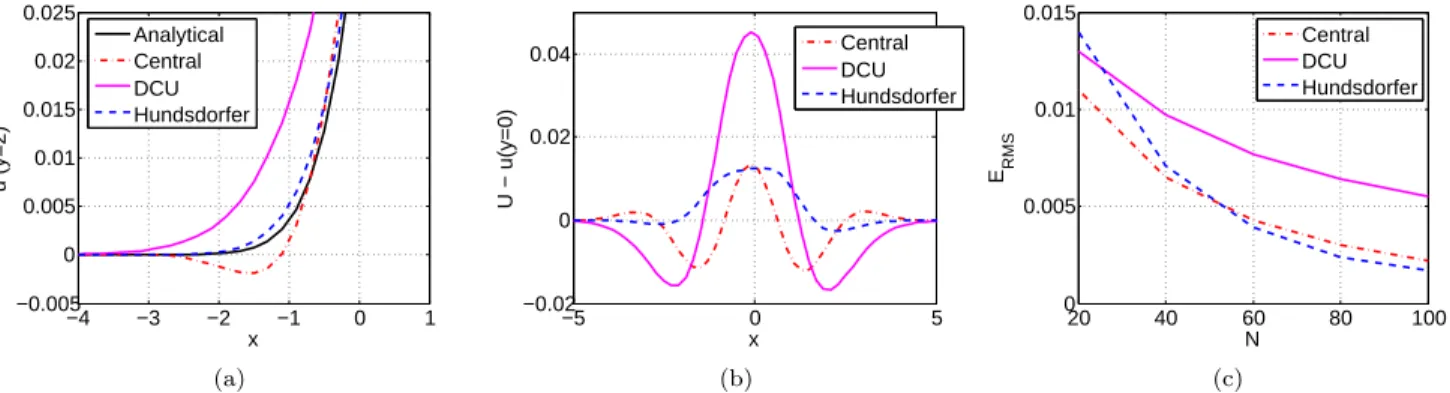
to obtainun+1. Comparisons between the analytical and numerical solutions are shown in figure 1.
As expected, the central finite-difference scheme does not preserve positivity, while both the first-order DCU scheme (9) and second-order Hundsdorfer scheme (11 - 13) preserve positivity. The central finite-difference sceme is second-order accurate, while the DCU scheme is first-order accurate. The Hundsdorfer scheme transitions from first-order to second-order accuracy as the number of grid pointsN increase. For smallN the grid is very coarse, such that the flux limiter φ≈0 due to large variations between neighbouring nodes and the Hundsdorfer scheme reduces to the first-order DCU scheme. As the number of grid points increase, the variation between neighbouring nodes decreases, the function becomes smoother, and φ→1, such that the Hundsdorfer scheme becomes second-order accurate.
−4 −3 −2 −1 0 1
−0.005 0 0.005 0.01 0.015 0.02 0.025
x
u (y=2)
Analytical Central DCU Hundsdorfer
(a)
−5 0 5
−0.02 0 0.02 0.04
x
U − u(y=0)
Central DCU Hundsdorfer
(b)
20 40 60 80 100
0 0.005 0.01 0.015
N ERMS
Central DCU Hundsdorfer
(c)
Figure 1: (a) The comparison of the analytical solution to numerical approximations shows that the central finite-difference scheme does not preserve positivity, while the other schemes do. (b) The difference between the analytical solution and numerical approximations fory= 0, withN= 100 grid points, shows that the second-order central finite-difference and Hundsdorfer schemes are more accurate than the first-order DCU scheme, a fact further illustrated by (c) the comparison of ERMS for the various numerical methods as a
function of the number of grid pointsN.
3. Fokker-Planck collision operator in cylindrical coordinates
The Fokker-Planck collision operator describes the local collisional relaxation process of distribution functions in plasmas under the assumption of binary, small-angle collisions [11, 12, 13] and is regarded, along with Vlasov and Maxwell’s equations, as the basis for weakly-coupled plasmas in all collisionality regimes. It conserves particle number, momentum and energy, preserves positivity of the distribution function, and satisfies the Boltzmann H-theorem, such that the steady-state solution is given by the Maxwellian distribution function. Despite this, however, it is a stiff advection-diffusion operator in velocity space, and nonlinear when solving the collision operators using the Landau integral [12] or the Rosenbluth potentials [11], which leads to several difficulties in dealing with it numerically [1].
In the presence of a strong magnetic field, the gyrofrequency exceeds all frequencies of interest, such that the dependence of the distribution function on the gyroangle can be neglected. The Fokker-Planck collision operator is normally solved in spherical coordinates (v, θ) where it contains no mixed derivative terms. In some cases, however, the distribution function must be solved under multiple effects, some of which may be best described in cylindrical coordinates (vk, v⊥), such as radiofrequency current drive [14, 15, 16], and an approximation to the collision operator in cylindrical coordinates is therefore required. The Fokker-Planck collision operator in cylindrical coordinates is therefore considered,
∂f ∂t =
1
v⊥ ∂ ∂v⊥v⊥
D⊥⊥ ∂f
∂v⊥ +D⊥k ∂f
∂vk −F⊥f
+ ∂
∂vk
Dkk ∂f
∂vk +Dk⊥ ∂f ∂v⊥ −Fkf
(17)
isotropic, background Maxwellian [15]. This assumption implies that energy will only be conserved if the distribution collides with a background Maxwellian; otherwise only particle number will be conserved, while the preservation of positivity is ensured by the numerical scheme. In general, the collision operators could be determined from the Landau integral [12] or the Rosenbluth potentials [11], but this is not considered in this work.
The solution to the Fokker-Planck equation (17) is obtained using the positivity-preserving scheme discussed earlier, but using the first-order DCU scheme for solving the advective equations. This simplifies the extension of the Chang and Cooper scheme, which ensures the correct equilibrium solution under the assumption of local thermal equilibrium. The result is a first-order solution that always conserves particle number and preserves positivity, while energy is conserved if the assumptions in calculating the collision operator are satisfied.
3.1. δ-splitting
The equilibrium solution to the collision operator is a Maxwellian distribution function, which is a strongly (ex-ponentially) varying function ofv. Central finite-difference schemes require a very fine grid in order to accurately resolve this strongly varying nature of the Maxwellian distribution, therefore Chang and Cooper [8] introduced a weighted averaging scheme which ensures the preservation of positivity and the conservation of particle num-ber. This scheme has been extended to two-dimensions, but the resulting approximation does not guarantee the preservation of positivity [9].
Here, we employ a similar weighted averaging scheme, but, as we employ a flux-conserving scheme for discretizing the advection-diffusion equation, particle number is conserved by construction. In this case, the assumption of local thermal equilibrium ensures the correct steady-state distribution and greatly improves the accuracy of the time evolution of the distribution function.
In general, the time evolution of the distribution function can be solved under multiple effects, such as collisions, electric fields and plasma-wave interactions [14, 15, 16], and this method could easily be extended to include these additional terms. Here, we only consider the effect of collisions, for which the Fokker-Planck equation can be written as the divergence of a flux,
∂f
∂t =∇ ·S~c
where the flux S~c will approach zero if the distribution is in steady-state. If the numerical scheme used for
approximating the time evolution of the distribution function does not guarantee the conservation of particle number under the divergence of a flux, then the assumptionS~c= 0 will ensure the conservation of particle number.
If the numerical scheme ensures the conservation of particle number by construction, however, as the flux-conserving scheme used in ths work, then the assumptionS~c= 0 will improve the accuracy of the numerical approximation to
the distribution function, as will be shown later.
The scheme introduced by Chang and Cooper therefore assumes local thermal equilibrium andS~c= 0, in order
to ensure the conservation of particle number. This condition can be used to derive a weighting parameter for the advective terms of the two-dimensional collision operator in cylindrical coordinates,Fk andF⊥.
First, consider thev⊥ part of the collision operator (17),
∂f ∂t =
1
v⊥ ∂ ∂v⊥v⊥
D⊥⊥ ∂f
∂v⊥ +D⊥k ∂f
∂vk −F⊥f
for which the flux,
D⊥⊥ ∂f
∂v⊥ +D⊥k ∂f
∂vk −F⊥f (18)
will equal zero if the distribution is in local thermal equilibrium. Under this assumption, the flux can be rewritten as
∂f ∂v⊥ =
1
D⊥⊥
F⊥−D⊥k·g
f (19)
where
g= 1
f ∂f
∂vk (20)
is equivalent to equation (14). Equation (19) can be discretized to obtain the solution
fi,j+1∼fi,jexp
F⊥
−D⊥k·g D⊥⊥ ∆v⊥
=fi,jexp
Ag−Bg
where the labels (i, j) refers to theith node in the parallel direction and thejthnode in the perpendicular direction. The functions Ag andBg are defined as
Ag=
F⊥
D⊥⊥∆v⊥ ; Bg=
D⊥k·g
D⊥⊥ ∆v⊥ (22)
The aim is to write the discretized form of theF⊥-term (forF⊥<0), using the first-order DCU scheme, as
∂f ∂t =
1 ∆v
v⊥−∆v/2
v⊥
F⊥
vk, v⊥−∆v
2
δ⊥fi,j
−
v⊥+ ∆v/2
v⊥
F⊥
vk, v⊥+∆v 2
δ⊥fi,j+1
by introducing, and solving, for δ⊥. The discretized form of the flux in the v⊥-direction (18), after rewriting the mixed derivative as an advective equation using (20) and the first-order DCU scheme for discretizing the advection equations, gives
1
∆pD⊥⊥,j+1/2(fi,j+1−fi,j) +D⊥k,j+1/2·gj+1/2·fi,j+1−F⊥,j+1/2·fi,j+1·δ⊥= 0
⇒fijeAge−Bg−fij+BgfijeAge−Bg−AgeAge−Bgfijδ⊥= 0
at the (v⊥+ ∆v/2)-boundary, forD⊥k·g >0. It equals zero under the assumption of local thermal equilibrium, and therefore,
δ⊥= 1
Ag
1 +Bg−e−AgeBg
(23)
with the same result obtained at the (v⊥−∆v/2)-boundary. ForD⊥k·g <0 (andF⊥<0), the solution toδ⊥ is given by
δ⊥= 1
Ag
1 +Bge−AgeBg−e−AgeBg
(24)
withAgandBggiven by (22). A similar approach is used for the flux in thevk-direction in order to obtain solutions
forδk, but in this case there are four possibilities,
Fk Dk⊥·h δk
>0 >0 1
Ah
eAh−Bh+B
heAh−Bh−1
<0 >0 1
Ah
1 +Bh−eBh−Ah
>0 <0 1
Ah
eAh−Bh−1 +B
h
<0 <0 1
Ah
1−eBh−Ah+B
heBh−Ah
with the functions Ah andBh defined as
Ah=
Fk
Dkk∆vk ; Bh=
Dk⊥·h Dkk ∆vk
and
h(vk, v⊥) = 1
f ∂f ∂v⊥
which is equivalent to equation (14).
3.2. Numerical stability
The δ-splitting method has been introduced to ensure the steady-state solution of the electron distribution function under the effect of only the Fokker-Planck collision operator is a Maxwellian distribution, due to the distribution being a strongly (exponentially) varying function of v. The introduction of δ, however, leads to a stability issue. Consider, for example, iff is a Maxwellian,
f ∼exp (−v2)
and therefore
g∼ −v
In the limitv→ ∞, we have A→0, but B→ ∓∞, such thatδ→ ∞. Numerically, this introduces problems, as large terms lead to instabilities by creating ill-conditioned matrices. The value of δ must therefore be limited to some maximumδmax. Fortunately there is the competing effect thatδ→1 for increasingN, such that, ifN is large enough, the value ofδmaxis irrelevant asδis always small enough for a stable solution, while the cutoff value
δmax only comes into effect at largev where there are very few particles.
As an example, consider the case of an initial Maxwellian distribution with Te= 20 eV colliding with a fixed
background distribution at Tb = 10 eV with densityne = 1014m−3. The number of grid points (N = 150 such
that vt= 10∆v) is chosen in order to demonstrate the effect ofδmax, as increasing the number of grid points can
eliminate the need for δmax.
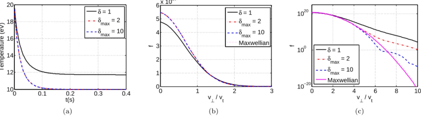
The temperature evolution reaches equilibrium att= 0.4 s. However, as electrons at largevcollide infrequently, the distribution functions only reach equilibrium at t = 1 s. As there are very few electrons at large v, the temperature does not change markedly after the bulk electrons reach equilibrium at t = 0.4 s. The temperature evolution up tot= 0.4 s and the distribution functions att= 1 s are therefore compared in figure 2 for three cases. Without δ-splitting (δ= 1), the wrong equilibrium temperature is reached, while for δmax = 2 and forδmax= 10 there are no differences in the temperature evolution, and the correct equilibrium temperature is reached, as expected, sinceδ-splitting ensures that the solution is a Maxwellian.
Comparing the distribution functions to the background distribution shows the effect ofδmax. Firstly, forδ= 1 the final distribution is different from the background distribution, due to the wrong equilibrium temperature being reached. Comparing theδmax= 2 andδmax= 10 distributions to the background distribution, it is clear that there are only small differences forv⊥<4vt, where the majority of electrons are, and therefore the correct temperature
is obtained. The differences are in the high v tail, with δmax = 2 underestimating the relaxation, and δmax = 10 overestimating the relaxation.
Larger values of δmax lead to ill-conditioned matrices as equilibrium is approached, so for numerical stability, the value ofδmax must be relatively small (δ≥1 always). Of course, asN→ ∞the value ofδ→1, and there will be no need for δmax. In practice, however, the grid will hardly ever be large enough to allow for this to happen, so it will be necessary to specify a value for δmax. Fortunately, this value will only impact regions of largev, where there are very few electrons which does not influence the low-order moments, such as temperature, and a relatively small value forδmaxsuffices.
0 0.1 0.2 0.3 0.4
10 12 14 16 18 20
t(s)
Temperature (eV)
δ = 1 δmax = 2 δ
max = 10
(a)
0 1 2 3
0 1 2 3 4 5 6x 10
20
v⊥ / v t
f
δ = 1 δmax = 2 δmax = 10 Maxwellian
(b)
0 2 4 6 8 10
10−20 100 1020
v⊥ / v t
f
δ = 1 δ
max = 2
δmax = 10 Maxwellian
(c)
Figure 2: (a) The time evolution of the temperature of an electron distribution function colliding with a fixed, background Maxwellian at Te = 10 eV andne = 10
14
m−3, for different choices ofδand δmax. There is no difference between the temperature curves for
δmax= 2 andδmax= 10. (b) The comparison of the steady-state distribution functions obtained shows no difference betweenδmax= 2,
3.3. Temperature equilibration
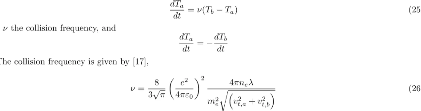
Consider two electron distributions of equal density colliding with each other. The distributions will equilibrate according to
dTa
dt =ν(Tb−Ta) (25)
withν the collision frequency, and
dTa
dt =− dTb
dt
The collision frequency is given by [17],
ν= 8 3√π
e2 4πε0
2
4πneλ
m2
e
r
v2
t,a+v2t,b
(26)
where v2
t,a= 2Ta/me is the thermal velocity of distributiona, and the Coulomb logarithm is taken to be constant
λ= 15.
Consider two distributions, with temperatures Ta = 20 eV andTb = 10 eV and densities na =nb = 1014m−3
colliding with each other. The resultant temperature evolution, when using δ-splitting, is shown in figure 3. Of course, the assumption that both distributions collide with a background Maxwellian is not always true; cold electrons undergo more collisions than warm electrons, such that cold electrons gain energy faster than warm electrons lose energy, and the distribution is not always Maxwellian, resulting in the wrong equilibrium temperature, as energy is not conserved.
By constraining both distributions to always be Maxwellian (by replacing each distribution with a Maxwellian of the same temperature at each time step), the assumption of collisions with a background Maxwellian remains true, and the correct equilibrium temperature is reached at the predicted rate, while energy is conserved.
If the collision operators are calculated through the Rosenbluth potentials [11] or the Landau integrals [12], it will no longer be necessary to constrain the distributions to be Maxwellian, as this constraint is only necessary to ensure the assumption of background Maxwellians is satisfied. The calculation of the collision operators from the distribution functions, however, adds additional numerical evaluations, and therefore is not considered here.
0 20 40 60 80 100
10 12 14 16 18 20
t(ms)
Temperature (eV)
Analytical
Numerical (Maxwellian) Numerical
(a)
0 20 40 60 80 100
−600 −400 −200 0 200 400 600
t(ms)
dTe / dt (eV.s
−1
)
Analytical
Numerical (Maxwellian) Numerical
(b)
Figure 3: The time evolution of (a) the temperature and (b) the temperature gradient for two Maxwellian distributions of density ne= 10
14
m−3colliding with each other, compared to the analytical temperature evolution. By constraining the distribution functions
to be Maxwellian, agreement with the analytical temperature is found, while the wrong equilibrium temperature is found otherwise.
3.4. Time evolution
number of grid points is N = 150, such that vt = 10∆v, while the densityne = 1014m−3 and the collision time
τ ≈20 ms.
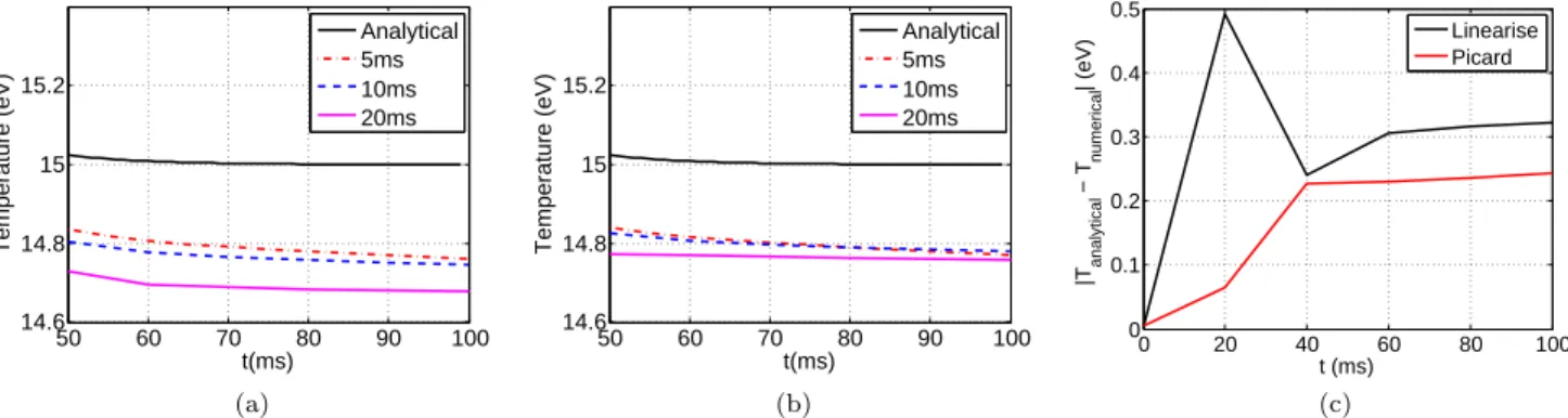
The time evolution of the temperature for different values of ∆tis shown in figure 4. As expected, convergence is achieved for larger time steps when approximating the time evolution of the distribution function through Picard iteration as compared to Picard linearizing. However, obtaining a solution through Picard iteration is computationally more expensive as we have to iterate over the solution fn+1.
50 60 70 80 90 100
14.6 14.8 15 15.2
t(ms)
Temperature (eV)
Analytical 5ms 10ms 20ms
(a)
50 60 70 80 90 100
14.6 14.8 15 15.2
t(ms)
Temperature (eV)
Analytical 5ms 10ms 20ms
(b)
0 20 40 60 80 100
0 0.1 0.2 0.3 0.4 0.5
t (ms)
|Tanalytical
− T
numerical
| (eV)
Linearise Picard
(c)
Figure 4: The time evolution of the temperature of a distribution function atTa= 20 eV colliding with a distribution atTe= 10 eV, both with densityne= 10
14m−3, for different choices of ∆twhen solving the distribution through (a) Picard linearizing and (b) Picard
iterating. (c) The comparison of the difference between the analytical and numerical temperatures for the two methods for ∆t= 20 ms, shows that Picard linearizing leads to more accurate approximations.
4. Conclusion
Lower-order numerical methods are less accurate, but generally more robust and reliable, than higher-order methods, which tend to be more complicated. In this paper we propose a scheme that focuses on improving the accuracy of lower-order methods, in particular with respect to the preservation of positivity, for solving two-dimensional advection-diffusion equations of the form
∂u ∂t =∇ ·
−~au+ ˆk· ∇u
whereu=u(x, y, t) is advected by the vector~a(x, y, t) and diffused by the tensor ˆk(x, y, t). Numerical solutions to these equations, in the absence of mixed derivatives, have been studied in detail [2, 3], but solutions of problems where mixed derivative terms are present have received much less attention. The scheme proposed in this paper allows the mixed derivative terms to be written as advection-type equations, after which a lower-order positivity-preserving scheme can be applied. It was discussed by using an example and then applied to the Fokker-Planck collision operator in cylindrical coordinates. Compared to central finite-difference methods, the proposed scheme obtains the same order of accuracy, with the added advantage of the solution being non-negative.
In our text core, the Fokker-Planck collision operator is approximated under the assumption of local thermal equilibrium, which introduces an averaging parameter to ensure an accurate steady-state distribution. The solution is tested with the thermal equilibration of two colliding Maxwellian distributions and compares well with the theoretically predicted rate. The scheme conserves particle number and preserves positivity, but only conserves energy and agrees with the theoretical equilibration rate if the distributions are constrained to be Maxwellian, as the collision operators are calculated under the assumption of a background Maxwellian.
The treatment of the mixed derivatives introduces a non-linearity, which can be solved through Picard iteration. This iteration allows for larger time steps to be taken, but also increases the computational time. For the considered example of studying the thermal equilibration of two electron distribution functions under the Fokker-Planck collision operator, Picard linearizing provides an accurate approximation to the time evolution when the time-step is shorter than the collision time.
which is less complicated than higher-order methods. The δ-splitting method can, in general, be applied to any advection-diffusion problem to ensure the correct steady-state solution. We show that, for equilibration under the Fokker-Planck collision operator, the scheme ensures the correct equilibrium distribution while conserving particle number and preserving positivity, while energy can be conserved by calculating the collision operators from the Rosenbluth potentials [11] or the Landau integral [12].
Acknowledgements
This work was funded by the RCUK Energy Programme under grant EP/P012450/1, and the University of York, through the Department of Physics and the WW Smith Fund. This work made use of the York Advanced Research Computing Cluster (YARCC) at the University of York.
References
[1] W.T. Taitano, L. Chac´on, A.N. Simakov and K. Molvig,J. Comput. Phys.297(2015) 357-380.
[2] R. Fazio and A. Jannelli,IAENG Int. J. Appl. Math. 39(2009) 1-11.
[3] W. Hundsdorfer, B. Koren, M. van Loon and J.G. Verwer, J. Comp. Phys.117(1995) 35-46.
[4] H.T. Huynh,18th AIAA Conference Paper 2007-4079 (2007) 1-42.
[5] T.D. Arber and R.G.L. Vann,J. Comp. Phys.180(2002) 339-357.
[6] E. Fijalkow,Comp. Phys. Comm.116(1999), 319-328.
[7] C.B. Laney, Computational Gasdynamics (Cambridge University Press, 1998).
[8] J.S. Chang and G. Cooper, J. Comp. Phys.6(1970) 1-16.
[9] E.S. Yoon and C.S. Chang,Phys. Plasma 21, 032503 (2014) 1-14.
[10] R. Courant, K. Friedrichs and H. Lewy Math. Ann.100(1928) 32-74.
[11] M.N. Rosenbluth, W.M. MacDonald and D.L. Judd,Phys. Rev.107(1957) 1-6.
[12] L.D. Landau,Zh. Eksper. i Theoret. Fiz. 7(1937) 203-209.
[13] S. Chandrasekhar,Rev. Modern Phys. 15(1943) 1-89.
[14] M.R. O’Brien, M. Cox and D.F.H. Start,Nucl. Fusion 26(1986) 1625-1640.
[15] C.F.F. Karney, Comput. Phys. Rep.4(1986) 183-244.
[16] T. Maekawa, T. Yoshinaga, M. Uchida, F. Watanabe and H. Tanaka, Nucl. Fusion 52, 083008 (2012) 1-19.
[17] J. Callen, Fundamentals of Plasma Physics (2006) [ebook]