A numerical technique based on integrated RBFs for the system evolution in molecular dynamics

A numerical technique based on integrated RBFs for

the system evolution in molecular dynamics

N. Mai-Duy

_{, T. Tran-Cong}

_{and N. Phan-Thien}

1

_{Computational Engineering and Science Research Centre}

Faculty of Engineering and Surveying,

University of Southern Queensland, Toowoomba, QLD 4350, Australia

2

_{Department of Mechanical Engineering}

Faculty of Engineering

National University of Singapore, Singapore

∗_{Corresponding author: E-mail [email protected], Telephone +61 7 4631 1332, Fax +61 7}

Abstract This paper presents a new numerical technique for solving the evolution

equa-tions in molecular dynamics (MD). The variation of the MD system is represented by

radial-basis-function (RBF) equations which are constructed using integrated multiquadric

basis functions and point collocation. The proposed technique requires the evaluation of

forces once per time step. Several examples are given to demonstrate the attractiveness

of the present implementation.

Key words: molecular dynamics, time evolution equation, numerical solver, radial basis

functions

1

Introduction

Based on the criterion of timescale, fluid simulations can be categorised into three regions:

atomistic (of the order of nanoseconds), mesoscopic (microseconds) and macroscopic

(sec-onds). On a macroscopic scale, a fluid can be modelled as a continuum and its motion

is adequately described by the Navier-Stokes equations which can be solved by

tradi-tional discretisation techniques such as finite-difference and finite-volume methods (e.g.

Roache, 1980). On a microscopic scale, one can employ molecular dynamics (MD)

simu-lation methods, which allow all of the actual atoms to be represented explicitly, thus to

have the ability to provide very detailed information about the behaviour of complex fluid

systems (e.g. Haile, 1992; Leach, 2001; Rapapport, 2004). On a mesoscopic scale,

simu-lations can be conducted using dissipative particle dynamics (DPD), where each particle

is regarded as a group of molecules (e.g. Espanol and Warren, 1995; Marsh, 1980).

In MD and DPD, a large number of particles are usually required. The time evolution of

particles is described by the Newton’s equations of motion which can be solved

numeri-cally. The essential idea of numerical methods is that the time domain is represented by

has been made to derive effective and efficient numerical schemes for the evolution of the

particle system.

Radial basis function networks (RBFNs) have emerged as a powerful numerical tool for the

solution of differential equations (e.g. Fasshauer, 2007). These approximators are able

to work well (i.e. providing fast convergence) with gridded and scattered data points.

The RBF approximations can be constructed through differentiation (DRBFNs) (e.g.

Kansa, 1990) or integration (IRBFNs) (e.g. Mai-Duy and Tran-Cong, 2001; Mai-Duy and

Tran-Cong, 2003; Mai-Duy, 2005). The latter has the ability to avoid the reduction in

convergence rate caused by differentiation and to provide an effective way of implementing

derivative boundary values.

This study is concerned with the application of IRBFNs for solving the evolution equations

in MD. The paper is organised as follows. A brief review of traditional numerical solvers

is given in Section 2. The proposed IRBF method is described in Section 3 and then

verified numerically in Section 4. Section 5 concludes the paper.

2

Traditional numerical solvers

The equations of motion of particles can be simply written in the form

¨

φ(t) =F(φ(t)) (1)

where φ is the field variable representing a component of the position vector; t the time;

F a known function; and dots represent derivatives with respect to time. In solving (1),

the evaluation ofF (force) is known to dominate the computational time. Any numerical

solver for the MD equations should be designed to keep the number of force evaluations

require the evaluation of forces once per time step, have been widely used in MD.

2.1

Verlet-based methods

The original Verlet algorithm (Verlet, 1967) can be described as

φ(t+h) = 2φ(t)−φ(t−h) +h2

F(φ(t)) (2)

where h denotes the size of the time step used for the numerical integration.

Implementation of (2) is straightforward. However, its RHS is the sum of a term of

order h2

and terms of order h0

. As a result, only a few significant figures of F(φ(t)) are

actually utilised, which may lead to a loss of precision. There is also the lack of an explicit

velocity term in the equation and one thus has to face difficulties in certain applications.

The velocity can be evaluated using the following approximation

˙

φ(t) = φ(t+h)−φ(t−h)

2h (3)

which is only carried out after the position at the next time step is obtained. The following

modified Verlet algorithms eliminate these types of problems.

Leap-frog algorithm: (Hockney, 1970)

˙

φ(t+h/2) = ˙φ(t−h/2) +hF(φ(t)) (4)

Velocity Verlet algorithm: (Swope et al., 1982)

φ(t+h) =φ(t) +hφ˙(t) + (h2

/2)F(φ(t)) (6)

˙

φ(t+h) = ˙φ(t) + (h/2) [F(φ(t)) +F(φ(t+h))] (7)

2.2

Predictor-corrector integration methods

The predictor-corrector methods typically involve three basic steps (Gear, 1971). First,

new positions, velocities, etc., are predicted using the values of the past

φ(t+h) = φ(t) +hφ˙(t) +h2

k−1

X

i=1

αiF(φ(t+ [1−i]h)) (8)

hφ˙(t+h) = φ(t+h)−φ(t) +h2

k−1

X

i=1

α′_iF(φ(t+ [1−i]h)) (9)

Second, the forces are evaluated at the new positions to give accelerations F(φ(t+h)).

Third, by taking into account the difference between the predicted and computed

accel-erations, the positions, velocities, etc., are corrected through

φ(t+h) = φ(t) +hφ˙(t) +h2

k−1

X

i=1

βiF(φ(t+ [2−i]h)) (10)

hφ˙(t+h) = φ(t+h)−φ(t) +h2

k−1

X

i=1

In (8)-(11), αi, α

′

i, βi and β

′

i are the coefficients that satisfy

k−1

X

i=1

(1−i)qαi =

1

(q+ 1)(q+ 2), q = 0,1,· · · , k−2 (12)

k−1

X

i=1

(1−i)qα′_i = 1

q+ 2 (13)

k−1

X

i=1

(2−i)qβi =

1

(q+ 1)(q+ 2) (14)

k−1

X

i=1

(2−i)qβ_i′ = 1

q+ 2 (15)

In the case of k = 4, {αi}

3

i=1 = 1/24× {19,−10,3}, {α ′

i}

3

i=1 = 1/24× {27,−22,7},

{βi}

3

i=1 = 1/24× {3,10,−1} and {β ′

i}

3

i=1 = 1/24× {7,6,−1}. It is noted that the force

function F is evaluated using the results of the predictor step rather than the corrected

values. Variations of this method include applying the corrector more than once.

3

Proposed IRBF technique

In this section, a numerical procedure based on IRBFNs and point collocation for the

solution of (1) on a set of points is presented. Integration constants arising from the

RBF construction process allow more preceding information to be incorporated into the

discrete system for the solution at the next time level.

3.1

Constructing the approximations

Second-order derivative of φ is decomposed into RBFs

¨

φ(t) =

n

X

i=1

where {wi}n_i=1 is the set of network weights and {gi(t)}

n

i=1 the set of RBFs. Expressions

for the first-order derivative and function itself are then obtained through integration

˙

φ(t) =

n

X

i=1

wiHi(t) +c1 (17)

φ(t) =

n

X

i=1

wiH¯i(t) +c1t+c2 (18)

where Hi(t) =

R

gi(t)dt, H¯i(t) =

R

Hi(t)dt and (c1, c2) are the constants of integration.

A distinguishing feature here is that the present coefficient vector, (w1,· · · , w_n, c1, c2)T,

is larger than that, (w1,· · · , w_n)T, of the conventional/differential approach.

3.2

Discretising the equations of motion

We implement two IRBFN versions, namely 2-point and 4-point schemes, which

cor-respond to, in terms of nodes, Verlet-based and predictor-corrector (k = 4) methods,

respectively. It can be seen that the values ofφ, ˙φand ¨φatt,t−h, t−2h, etc., are given.

Our objective here is to find the values of φ, ˙φ and ¨φ at t+h.

3.2.1 Two-point IRBFN scheme

The IRBFN approximations are constructed over two points (n= 2), t and t+h. Owing

to the presence of the integration constants, one can incorporate not only φ(t) and ¨φ(t)

but also ˙φ(t) into the IRBFN system in an exact manner



    

φ(t)

¨

φ(t)

˙

φ(t)



    

=A1



       

w1

w2

c1

c2



       

where A1 is defined as

A1 =

      ¯

H1(t), H¯2(t), t, 1

g1(t), g2(t), 0, 0

H1(t), H2(t), 1, 0

      (20)

Solving (19) gives

         w1 w2 c1 c2         

=A−1

1      

φ(t)

¨

φ(t)

˙

φ(t)

      (21)

The new position is then obtained

φ(t+h) = [ ¯H1(t+h),H¯2(t+h), t+h,1]A− 1 1      

φ(t)

¨

φ(t)

˙

φ(t)

      (22)

from which one can calculate the new acceleration ¨φ(t+h) using (1).

To compute ˙φ(t+h), an IRBFN system is constructed as follows

        

φ(t+h)

¨

φ(t+h)

¨

φ(t)

˙

φ(t)

        

=A2

         w1 w2 c1 c2          (23)

where A2 is defined as

A2 =

         ¯

H1(t+h), H¯2(t+h), t+h, 1

g1(t+h), g2(t+h), 0, 0

g1(t), g2(t), 0, 0

H1(t), H2(t), 1, 0

In (23), there are four values included instead of the usual two. These values are imposed

exactly owing to the presence of c1 and c2.

The value of the new velocity is then determined through

˙

φ(t+h) = [H1(t+h), H2(t+h),1,0]A− 1 2         

φ(t+h)

¨

φ(t+h)

¨

φ(t)

˙

φ(t)

         (25)

3.2.2 Four-point IRBFN scheme

The IRBFN approximations are constructed over four points (n = 4),{t−2h, t−h, t, t+h}.

The solution procedure is similar to that of the 2-point IRBFN scheme. The IRBFN

approximations for the position and velocity are of the forms

           

φ(t−2h)

¨

φ(t−2h)

¨

φ(t−h)

¨

φ(t)

˙

φ(t)

           

=A1

                w1 w2 w3 w4 c1 c2                 (26)                

φ(t+h)

¨

φ(t+h)

¨

φ(t)

¨

φ(t−h)

¨

φ(t−2h)

˙

φ(t)

               

=A2

where

A1 =

            ¯

H1(t−2h), H¯2(t−2h), H¯3(t−2h), H¯4(t−2h), t−2h, 1

g1(t−2h), g2(t−2h), g3(t−2h), g4(t−2h), 0, 0

g1(t−h), g2(t−h), g3(t−h), g4(t−h), 0, 0

g1(t), g2(t), g3(t), g4(t), 0, 0

H1(t), H2(t), H3(t), H4(t), 1, 0

            (28) and

A2 =

                ¯

H1(t+h), H¯2(t+h), , H¯3(t+h), H¯4(t+h) t+h, 1

g1(t+h), g2(t+h), g3(t+h), g4(t+h), 0, 0

g1(t), g2(t), g3(t), g4(t), 0, 0

g1(t−h), g2(t−h), g3(t−h), g4(t−h), 0, 0

g1(t−2h), g2(t−2h), g3(t−2h), g4(t−2h), 0, 0

H1(t), H2(t), H3(t), H4(t), 1, 0

                (29)

The IRBFN formulas for computing the new position and velocity thus become

φ(t+h) = [ ¯H1(t+h),H¯2(t+h),H¯3(t+h),H¯4(t+h), t+h,1]A− 1 1            

φ(t−2h)

¨

φ(t−2h)

¨

φ(t−h)

¨

φ(t)

˙

φ(t)

            (30) ˙

φ(t+h) = [H1(t+h), H2(t+h), H3(t+h), H4(t+h),1,0]A− 1 2                

φ(t+h)

¨

φ(t+h)

¨

φ(t)

¨

φ(t−h)

¨

φ(t−2h)

˙

φ(t)

One common feature in the two present IRBFN schemes is that information about the

governing equation (1) is used as much as possible. For example, in (23) and (27), (1) is

collocated at every interpolation point.

With (18), (17) and (16), one is also able to observe the variation ofφ and its derivatives

between t and t+h. In the proposed technique, the approximations are of high order

and one is able to incorporate more preceding information into the discrete system in a

proper manner. Unlike the predictor-corrector method, the present value of φ at t+h is

unique. Since the values of φ, ˙φ and ¨φ at t+h are imposed at the same time ((23) and

(27)), their relations, i.e. ˙φ =dφ/dt and ¨φ=d2

φ/dt2

, are satisfied exactly.

It can be seen that the process of constructing the IRBFN approximations needs be done

only once. The resultant IRBF approximations can be used for every time step and for

every particle in the system. At each time step, the present technique requires one force

evaluation and the multiplication of matrices and vectors whose sizes are quite small.

4

Numerical Results

The present IRBFN schemes are implemented with the multiquadric (MQ) function whose

form is

gi(t) =

q

(t−ti)2+a2i (32)

where ti and ai are the centre and width of the ith MQ-RBF, respectively. The latter is

simply chosen according to the relation

ai =βh (33)

where β is a positive number. The RBF width can be used to influence the accuracy of

the other hand, the matrix condition number grows as the number of RBF centres and

the RBF width increase. This inter-dependence is known as the uncertainty or trade-off

principle. Fortunately, the number of MQ centres in the present schemes are relatively

low (only two and four) which allow larger values ofβ to be used here.

4.1

Example 1

Consider the following ODE of motion for a one-dimensional harmonic oscillator

¨

φ(t) = −(2π)2

φ(t) (34)

This problem was suggested as a simple exact test for molecular dynamics algorithms

(Venneri and Hoover, 1987). The analytic solution can be verified to beφe(t) = cos(2πt).

Calculations are carried out over 0≤t≤1 with various time steps

{1/10,1/14,1/18,1/22,· · · ,1/102}.

Tables 1 and 2 present the relative L2 error, denoted by N_e(φ), of the computed solution

obtained by different techniques.

Results by the 2-point IRBFN scheme (β = 16) are compared with those predicted by

the Verlet, leap-frog and velocity Verlet algorithms (Table 1).

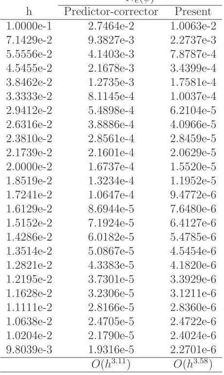
Results by the 4-point IRBFN scheme (β = 31) are compared with those obtained by

the predictor-corrector integration method with k = 4 (Table 2). Effect of β on the

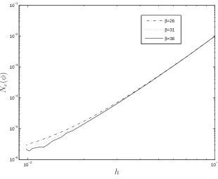
solution accuracy is investigated in Figure 1, showing that the IRBFN results are not

much different for various large values of β.

It can be seen that the present schemes gives superior accuracy and faster convergence

4.2

Example 2

Consider a three-dimensional system of MD particles which is allowed to evolve to

equi-librium. We adopt the Weeks-Chandler-Anderson (WCA) potential, i.e. a modification

of the Lennard-Jones potential,

u(rij) = 4ε

"

σ rij

12

−

σ rij

6#

+ε, rij < rc = 2

1_/6

σ (35)

whererij =krijk, in whichrij =ri−rj and ri and rj are the position vectors of particles

i and j, respectively, ε is a parameter characterising the strength of the interaction, σ

the molecular length scale and rc the cut-off distance, i.e. u(rij) = 0 when rij ≥ rc.

Parameters used here are the same as those in Problem 1 (Chapter 3) (Rapaport, 2004).

We employ an array of 5×5×5 unit cells and the density of 0.8. The initial state is a

simple cubic lattice so that the system involves 125 particles. Simulations are carried out

with several time steps. For comparison purposes, the leap-frog and predictor-corrector

(k = 4) methods are also employed.

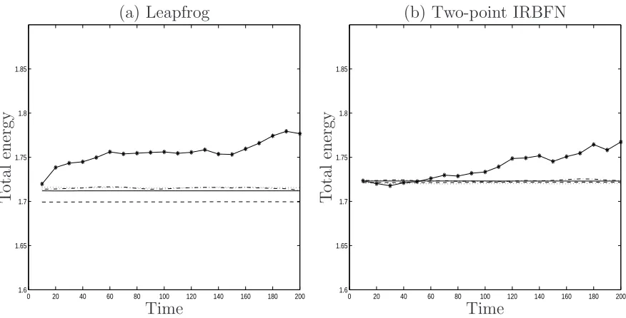
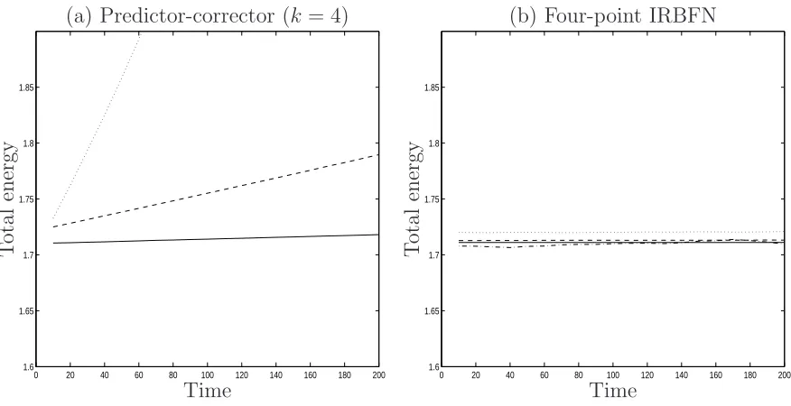
Results concerning energy conservation are presented in Figures 2 and 3. A total run

involves 200 time units and results are stored at every ten time units. In the case of

two-point discretisations (Figure 2a), the two-point IRBFN scheme (β = 16) and the

leap-frog method both perform well. The total energy is well conserved with time for a

wide range of time step from 0.00125 to 0.01 and slightly increases for a large time step

of 0.02. In the case of four-point discretisations (Figure 2b), for a given degree of energy

conservation, large time steps can be used with the proposed scheme. For the

predictor-corrector method, there are noticeable increases in the total energy with time for time

steps of 0.0025 and 0.005. In contrast, the 4-point IRBFN scheme (β = 31) works well

5

Concluding remarks

In this paper, a new numerical technique for solving the evolution equations in molecular

dynamics is presented. The proposed technique is based on high-order integrated RBFs

and point collocation. For a given number of interpolation points, the proposed technique

has the ability to incorporate more preceding information owing to the presence of the

constants of integration. Numerical examples show that the proposed technique is more

accurate and stabler than traditional techniques.

Acknowledgement

This work is supported by the Australian Research Council.

References

1. P. Espanol and P.B. Warren, Statistical mechanics of dissipative particle dynamics,

Europhysics Letters, 30(4): 191-196 (1995)

2. Fasshauer, G.E. (2007). Meshfree Approximation Methods With Matlab

(Interdisci-plinary Mathematical Sciences - Vol. 6). World Scientific Publishers, Singapore.

3. Gear C W (1971) Numerical Initial Value Problems in Ordinary Differential

Equa-tions. Englewood Cliffs, NJ, Prentice Hall

4. J. M. Haile (1992) Molecular Dynamics Simulation: Elementary Methods. New

York: John Wiley & Sons

5. R. W. Hockney (1970) The potential calculation and some applications. Methods

6. Kansa, E.J. (1990). Multiquadrics- A scattered data approximation scheme with

applications to computational fluid-dynamics-II. Solutions to parabolic, hyperbolic

and elliptic partial differential equations. Computers and Mathematics with

Appli-cations, 19(8/9), 147–161

7. Leach, A.R. (2001)Molecular Modelling Principles and Applications. Harlow :

Pren-tice Hall

8. Mai-Duy, N. and Tran-Cong, T. (2001). Numerical solution of differential equations

using multiquadric radial basis function networks. Neural Networks, 14(2), 185–199.

9. Mai-Duy, N. and Tran-Cong, T. (2003). Approximation of function and its

deriva-tives using radial basis function networks. Applied Mathematical Modelling, 27,

197–220.

10. Mai-Duy N (2005) Solving high order ordinary differential equations with radial

ba-sis function networks. International Journal for Numerical Methods in Engineering,

62, 824–852

11. D.C. Rapapport (2004) Art of Molecular Dynamics Simulation. New York:

Cam-bridge University Press.

12. C. Marsh, Theoretical aspect of dissipative particle dynamics, PhD Thesis,

Univer-sity of Oxford, 1998

13. Roache, P.J. (1980). Computational Fluid Dynamics. Albuquerque: Hermosa

Pub-lishers.

14. W.C. Swope, H.C. Andersen, P.H. Berens and K.R. Wilson (1982) A computer

simulation method for the calculation of equilibrium constants for the formation of

physical clusters of molecules: Application to small water clusters. Journal Chemical

15. G.D. Venneri and W.G. Hoover (1987) Simple exact test for well-known molecular

dynamics algorithms, Journal of Computational Physics, 73(2), 468–475

16. L. Verlet (1967) Computer“experiments” on classical fluids. I. Thermodynamical

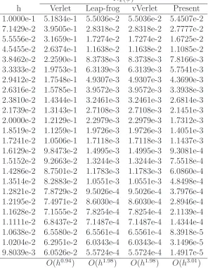
Table 1: 1D Harmonic oscillator, two interpolation points: discrete relativeL2 error

Ne(φ)

h Verlet Leap-frog vVerlet Present

1.0000e-1 5.1834e-1 5.5036e-2 5.5036e-2 5.4507e-2 7.1429e-2 3.9505e-1 2.8318e-2 2.8318e-2 2.7777e-2 5.5556e-2 3.1659e-1 1.7274e-2 1.7274e-2 1.6725e-2 4.5455e-2 2.6374e-1 1.1638e-2 1.1638e-2 1.1085e-2 3.8462e-2 2.2590e-1 8.3738e-3 8.3738e-3 7.8166e-3 3.3333e-2 1.9753e-1 6.3139e-3 6.3139e-3 5.7541e-3 2.9412e-2 1.7548e-1 4.9307e-3 4.9307e-3 4.3690e-3 2.6316e-2 1.5785e-1 3.9572e-3 3.9572e-3 3.3938e-3 2.3810e-2 1.4344e-1 3.2461e-3 3.2461e-3 2.6814e-3 2.1739e-2 1.3143e-1 2.7108e-3 2.7108e-3 2.1451e-3 2.0000e-2 1.2129e-1 2.2979e-3 2.2979e-3 1.7312e-3 1.8519e-2 1.1259e-1 1.9726e-3 1.9726e-3 1.4051e-3 1.7241e-2 1.0506e-1 1.7118e-3 1.7118e-3 1.1437e-3 1.6129e-2 9.8473e-2 1.4995e-3 1.4995e-3 9.3081e-4 1.5152e-2 9.2663e-2 1.3244e-3 1.3244e-3 7.5518e-4 1.4286e-2 8.7501e-2 1.1783e-3 1.1783e-3 6.0860e-4 1.3514e-2 8.2883e-2 1.0551e-3 1.0551e-3 4.8498e-4 1.2821e-2 7.8729e-2 9.5026e-4 9.5026e-4 3.7976e-4 1.2195e-2 7.4971e-2 8.6030e-4 8.6030e-4 2.8946e-4 1.1628e-2 7.1555e-2 7.8254e-4 7.8254e-4 2.1139e-4 1.1111e-2 6.8437e-2 7.1487e-4 7.1487e-4 1.4344e-4 1.0638e-2 6.5580e-2 6.5561e-4 6.5561e-4 8.3918e-5 1.0204e-2 6.2951e-2 6.0343e-4 6.0343e-4 3.1496e-5 9.8039e-3 6.0526e-2 5.5724e-4 5.5724e-4 1.4917e-5

O(h0_.94

) O(h1_.98

) O(h1_.98

Table 2: 1D Harmonic oscillator, four interpolation points: discrete relative L2 error

Ne(φ)

h Predictor-corrector Present

1.0000e-1 2.7464e-2 1.0063e-2

7.1429e-2 9.3827e-3 2.2737e-3

5.5556e-2 4.1403e-3 7.8787e-4

4.5455e-2 2.1678e-3 3.4399e-4

3.8462e-2 1.2735e-3 1.7581e-4

3.3333e-2 8.1145e-4 1.0037e-4

2.9412e-2 5.4898e-4 6.2104e-5

2.6316e-2 3.8886e-4 4.0966e-5

2.3810e-2 2.8561e-4 2.8459e-5

2.1739e-2 2.1601e-4 2.0629e-5

2.0000e-2 1.6737e-4 1.5520e-5

1.8519e-2 1.3234e-4 1.1952e-5

1.7241e-2 1.0647e-4 9.4772e-6

1.6129e-2 8.6944e-5 7.6480e-6

1.5152e-2 7.1924e-5 6.4127e-6

1.4286e-2 6.0182e-5 5.4785e-6

1.3514e-2 5.0867e-5 4.5454e-6

1.2821e-2 4.3383e-5 4.1820e-6

1.2195e-2 3.7301e-5 3.3929e-6

1.1628e-2 3.2306e-5 3.1211e-6

1.1111e-2 2.8166e-5 2.8360e-6

1.0638e-2 2.4705e-5 2.4722e-6

1.0204e-2 2.1790e-5 2.4024e-6

9.8039e-3 1.9316e-5 2.2701e-6

O(h3_.11

10−2 10−1 10−6

10−5 10−4 10−3 10−2 10−1

β=26 β=31 β=36

h Ne

(

φ

)

0 20 40 60 80 100 120 140 160 180 200 1.6

1.65 1.7 1.75 1.8 1.85

(a) Leapfrog

Time

T

ot

al

en

er

gy

0 20 40 60 80 100 120 140 160 180 200

1.6 1.65 1.7 1.75 1.8 1.85

(b) Two-point IRBFN

Time

T

ot

al

en

er

gy

0 20 40 60 80 100 120 140 160 180 200 1.6

1.65 1.7 1.75 1.8 1.85

(a) Predictor-corrector (k= 4)

Time

T

ot

al

en

er

gy

0 20 40 60 80 100 120 140 160 180 200

1.6 1.65 1.7 1.75 1.8 1.85

(b) Four-point IRBFN

Time

T

ot

al

en

er

gy