Stationary solution of the ring-spinning balloon in zero air drag using a RBFN based mesh-free method

Stationary Solution of the Ring-spinning Balloon in Zero Air

Drag using a RBFN based mesh-free Method

Canh-Dung Tran1, David G. Phillips2 and W. Barrie Fraser3 1,2 _{CSIRO Textile and Fibre Technology, Geelong, VIC 3216, Australia.} 3 _{School of Mathematics and Statistics, University of Sydney, NSW 2006, Australia.}

Abstract:A technique for numerical analysis of the dynamics of the ring-spinning balloon based on the Radial Basis Function Networks (RBFNs) is presented in this paper. This method uses a “universal approximator” based on neural network methodology to solve the differential governing equations which are derived from the conditions of the dynamic equilibrium of the yarn to determine the shape of balloon yarn. The method needs only a coarse finite collocation points without any finite element-type discretisation of the domain and its boundary for numerical solution of the governing differential equations. This paper will report a first assessment of the validity and efficiency of the present mesh-less method in predicting the balloon shape across a wide range of spinning conditions.

Keywords: Ring-Spinning balloon, Differential Governing Equations, Neural Networks, Radial Basis Function Networks (RBFNs).

1. Introduction

The theory of ring spinning has undergone development and refinement for several decades (Hannah, 1952, 1955; Mack, 1953; De Barr, 1958; Padfield, 1958; Kothari and Leaf, 1979; Batra et al., 1989a,b; Fraser, 1993; Fraser and Stump, 1998) with the modelling and analysis of the yarn balloon of special interest. The yarn balloon is generated by the rotation of the yarn loop from the guide eye and the traveller around a fixed axis of bobbin (Figure 1 and 5) and the dynamics of the whirling yarn has been studied extensively: Mack (1953) and Fraser (1993) studied theoretically the spinning balloon curve; Turteltaub and Bejar (1976) focussed on the stability of the yarn balloon; Batra et al. (1989a,b) gave the stationary numerical solutions of yarn balloon with and without air drag forces using a non-dimensional formulation. Fraser and his co-workers (Clark et al., 1998; Stump and Fraser, 1996) considered the dynamic response and the transient solutions of the spinning yarn balloon.

method does not require any fixed connectivity to satisfy a predetermined topology (i.e. a mesh in which the elements are constrained by some geometrical regularity conditions) but only a set of unstructured discrete collocation nodes in the analysis domain and on its boundary.

This paper describes the use of the Integral RBFN based mesh-free method to study the dynamics of ring-spinning balloon and organized as follows. In sections 2, the governing equation of the yarn balloon profile is represented based on the dynamics of yarn in ring-spinning balloon. The non-dimensional form is introduced to express the differential governing equation together with the boundary conditions of the problem. In section 3, the RBFN based numerical method for approximation of a function and the derivatives, is outlined. Especially the Integral RBFN based integration of the equation of motion of the balloon is represented. The algorithm of the method in solving the nonlinear governing equation of balloon is described. The results and evaluation are then discussed in section 5 with a brief conclusion in section 6.

2. Mathematical formulation of ring spinning

The dynamics of yarn spinning have been detailed in many studies (Hannah, 1952, 1955, Mack, 1953; Turteltaub and Bejar, 1976; Fraser, 1993; Batra et al. 1989a, b). The details of the engineering approach used in this work are given as follows.

2.1. Governing Equation of the Yarn Balloon

.

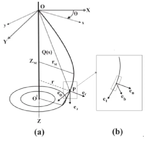
[image:2.612.183.431.334.578.2]

Considering the flexible and inextensible ring-spinning balloon in a fixed coordinated frame (0,X,Y,Z), let (0,x,y,z) be the moving coordinate frame where z coincides with the bobbin axis. Alternatively, a cylindrical polar coordinate system is also defined via unit vector er (radial outward), eθ (circumferential), and ez (parallel to the bobbin axis), Figure 1(a). Also, using the principal triad, each point of the yarn balloon can be expressed by a three component unit vector: the tangent to the yarn path (et), principal normal (en, normal to the yarn path) and bi-normal (eb), Figure 1(b).

Consider a small yarn segment of length ds (at the point P) in the moving frame with position Q(s) where s is the arc-length OP, see Figure 1(a). Neglecting the air drag and gravitational forces, the general equation of motion of this segment is given in the triad system by (Batra et al., 1989a)

(

2

)

n r

ds v r ds d

ρ = ω − ω ρ =

γ e e T (1)

where dT (T = Tet) is the tension of yarn balloon; ρ is the mass per unit length of the yarn; ωisthe constant angular velocity of the yarn balloon; r is the balloon radius at P, γ is the acceleration of the segment consisting of the centripetal acceleration

(

−ω2rer

)

and the Coriolis acceleration

(

ωven

)

in

which v is the input velocity of the yarn in the fixed coordinates. This Coriolis component is neglected because the rotational velocity of traveller is much higher than the input velocity v. By projecting equation (1) on et gives the equation describing the tension of balloon:

2

dT= −ω ρrdr (2)

The development of the equation of motion (1) in the cylindrical coordinates yields the governing equation of balloon shape as follows (Batra et al. 1989a, De Barr and Catling, 1965)

2

2 2

2 z

d r r dr

1 0

dz T dz

ρω  

+ +_{ } =

  (3)

where Tz is the component of T along the direction ez in the cylindrical coordinates. Furthermore, with zero air drag, Tz is constant along the yarn in the balloon and the balloon in the zero air drag case is a planar curve contained in an rz-plane. Let To be the tension of yarn balloon at the guide eye (z = 0; r = 0) (see Figure 1). Integrating equation (2) yields

2 2

o

T= − ω ρ +0.5 r T (4)

Thus, from (4) the yarn tension is dependent on the position of yarn balloon and the tension of yarn balloon is a maximum at the guide-eye (To).

2.2 Non-dimensionalisation

In this section, the variables are scaled and the above equations are rewritten in non-dimensional form. As well as the advantages mentioned in Fraser (1993), the dimensionless presentation also advantages the training process of the RBF based networks by reducing the round-off error as shown in Tran and Phillips, 2006). Here, the variables z, r and T are scaled by h, ro andρω2 2ro ,

respectively and the dimensionless variables are given by (Batra et al., 1989a; Padfield, 1958 and Fraser, 1993)

z Z

h = ;

o

r R

r = ; *

2 2 o

T T

r =

ρω (5)

Where h, ro are the balloon height and the ring radius, respectively; ρ is the mass per unit length of the yarn; ω is angular velocity of the traveller.

In order to consider the effect of the ratio of the ring radius (ro) to the balloon height (h) on the yarn balloon shape, the length variables r and z are scaled by two different values (Batra et al., 1989a). Three dimensionless parameter groups L = ro/h, P= ρω2 2r / To o and k = Tz/To are introduced and

2 2 2

2 2

d R P R dR

1 L 0

dZ L k dZ

   

+_{ } + _{ } =

    (6)

(

2 2

)

o

T

1 0.5P R

T = − (7)

2.3. Boundary Conditions in Stationary Ring-spinning

Since the balloon under consideration is uncontrolled (i.e., a free balloon), as a result of the stationary condition, the solution of the differential governing equation of balloon is obtained subject to the following boundary conditions in non-dimensional form

At the guide eye: R = 0 at Z = 0 (8)

At the traveller: R = 1 at Z = 1 (9)

Furthermore, if the balloon reaches a radius larger than that of the ring (R > 1) then there exists a maximum value RM between the guide eye and bottom position of balloon and an additional condition is also imposed that

M

dR

0 at Z Z

dZ = = (10)

where M M 0 r R r

= , and rM is the maximum value of balloon radius and considered as the radius of balloon at the first critical point (Batra et al., 1989a), Figure1(a). The tension Tz at the unknown location (ZM, RM) is the tension of the balloon. Equation (7) yields the ratio (k)

(

2 2

)

z

M o

T

k 1 0.5P R

T

= = − (11)

In the analysis, the tension To is assumed to be known. Tz depends on the tension To , related to the traveller mass, yarn linear density and operating conditions, and determines the shape of the balloon. From Equation (11), Equation (6) is rewritten by

(

)

2 2

2

2

2 2 2

M

d R P R dR

1 L 0

dZ L 1 0.5P R dZ

   

+_{ } + _{ } =

−

    (12)

3. RBFN based mesh-free method for solving the governing equation of balloon.

The application of RBFN’s in numerical solution of PDE's has brought interesting results (Kansa, 1990; Zerroukat et al., 1998; Tran-Canh and Tran-Cong, 2002b, 2004). After comparing many available interpolation methods for the analysis of scattered data, Franke (1982) ranked the Multi-quadric RBF (MQ-RBF) as superior in accuracy and this RBF is employed in the present work.

3.1 Review of the RBFN method

The present work uses the linear RBF based networks with one hidden layer where an arbitrary function f(x) can be decomposed into m fixed Radial Basis Functions as follows

( )

m j j

( )

j 1

f x w h x

=

where wj _{is the synaptic weight and h}j _{is the chosen radial basis function corresponding to the j}th neuron. Usually m ≤ n (Haykin, 1999) where n is the number of input data points (xi,y)i); xi is the coordinate of the ith collocation point and y)i is the desired value of function f(x) at the collocation point xi. In this work the multi quadric RBF is employed and given by

( )

(

)

( )j 2

j j j 2

h r =h x c− = r −a ₍₁₄₎

where r =(x -cj_{) and r=}

(

_x−cj

)

_{is the Euclidean norm of r; {c}j_{}is a set of centres that can be} chosen from among the data points; aj _{> 0 is the width of the j}th _{RBF. The accuracy of the} MQ-RBF approximation is dependent on the width of the MQ-RBF (Kansa, 1990a; Carlson and Foley, 1991), whose choice is still an open question. In the present work, the set of centres is chosen as same as the set of training collocation points. The width aj is computed as follows

j j _d

a =ς (15)

where dj _{is the distance from the j}th _{centre to the nearest centre; ς is a chosen coefficient. In the} conventional RBFN method (Hardy, 1971), after obtaining the RBFN based approximated function, its derivatives are determined by differentiating directly as follows

( )

( )

m j j m

j 1 j j

j 1

i i

m j j

2 _m

j 1 j j

j 1

i j j

w h ( ) f

w g ( )

x x

w g ( ) f

w k ( )

x x x

= = = = ∂ ∂ = = ∂ ∂ ∂ ∂ = = ∂ ∂ ∂

∑

∑

∑

∑

x x x x x

x ₍₁₆₎

where gj(x) and kj(x) are the first and second derivatives of the RBF hj(x).

3.2 The Integral RBFN method

In this method, the highest order derivative is expressed in terms of the RBFNs, and then the lower order derivatives and finally the function are determined by the successive integrations (Mai-Duy and Tran-Cong, 2001). In this work, the second derivative d R2₂

dZ of the balloon function R = f(Z) in Equation (12) is approximated by the RBFNs and then the first derivatives f / Z∂ ∂ and root function R = f(Z) can be calculated, respectively as follows

( )

( )

( )

( )

( )

( )

( )

2 _m j j 2 j 1 m m

j j j j

o

j 1 j 1

m j j

o 1

j 1

d f Z

w h Z , dZ

df Z

w h Z dZ w g Z C ,

dZ

R(Z) f Z w g Z dZ C Z C .

= = = = = = = + ≈ = + +

∑

∑

∫

∑

∑ ∫

(17a,b,c)

WhereCoandC1are integral constants and g

( )

( )

(

)

( )

( )

( )

( )

1

( )

( )

2 _{m m}

2

j j i j (i)2

2

j 1 i 1

m m

j j j j

o

j 1 j 1

m t m

j j j j

o 0 i 1

k 1 j 1

d f Z

w h Z w Z c a

dZ df Z

w h Z dZ w g Z C

dZ

R f Z w g Z C dZ w l Z C Z C

= = = = + = = = = − +   = _{ } = +     = = _ + _ = + +  

∑

∑

∑

∑

∫

∑

∑

∫

(18a,b,c)

where gj and lj are integrated directly from the MQ_RBF as follows successively

( )

( )

(

) (

)

(

) (

)

( )

( )

(

(

)

)

(

) (

)

(

)

j j ( j) _{( j)}

j j j j ( j)

.

j ( j)

( j)

j j j j ( j)

( j)

j ( j)

Z c Z c a _a

g Z h Z dZ ln Z c Z c a Z c a _a

l Z g Z dZ Zln Z c Z c a a

Z c a

− − + _{ } = = + _ − + − + _   − + _{ } = = + _ − + − + _   − − +

∫

∫

2 ₂ 2 ₂ 2 1 5 2 ₂ 2 2 ₂ 2 ₂ 2 2 2 6 2 2

3.3 Integrating the Governing Equation using the Integral RBFN method

This section describes the Integral RBFN-based numerical technique employed to solve the governing equations of the balloon shape (12) subject to the boundary conditions (8) and (9) which are repeated here

(

)

2 2

2

2

2 2 2

M

d R P R dR

1 L 0 dZ L 1 0.5P R dZ

   

+_{ } + _{ } =

−

    (12)

R = 0 at Z = 0 (8)

R = 1 at Z = 1 (9)

With a chosen set of collocation points (including the points in the analysis volume from the guide eye O to the ring centre O’, see Figure1(a), and on the boundaries), the substitution of the closed forms of Equations (18a,b,c) into the Equations (12), (8)-(9) gives the sum of the square error in the sense of the linear least square principle as follows

( )

(

)

( )

(

) (

)

max 2 2 2 2 2 2 1

i _{2 2} i i

i

d R dR

SSE Z R(Z ) 1 L Z R(0) 0 R(1) 1

dZ 1 P R dZ

∈Ω

 _{ρ  } 

 

= + + _{ } + − + −

 −   

 

∑

(22)

Where i denotes the ith collocation points Zi;

2

1

P L

 

ρ =  _{ } and Ω is set of collocation points included the boundary in this work. Note that there exists the nonlinear term _{1 L}2 dR 2

( )

_Z

dZ

 

+ _{ }

  and the

maximum value (Rmax) of the unknown function R which need to be processed using a special numerical treatment.

(a) The initial derivative values

( )

i

dR Z

dZ are guessed at the set of collocation points (zero values in

this work) and the maximum value of the function is attained at the traveller point (the boundary condition R(1) = 1).

(b) The nonlinear term in the second term of Equation (12) is linearised by using the current estimation of derivative function and maximum functional value but keeping the function R as unknown, i.e. at the tth iteration

( )

1/ 2 2 2

i

dR 1 L Z

dZ

 _{ } 

+

 _{ } 

 _{ } 

  is represented by

( )

1/ 2 2,t 1 i dR 1 Z dZ −  _{ }  +  _{ }   _{ } 

  and the

maximum value Rmax by Rt 1max

− _.

(c) Equation (22) is solved using the general linear least square principle to obtain a new estimation the function of the balloon profile and its derivative.

(d) The convergence measure (CM1) for the shape function at the tth iteration is calculated as defined as follows

(

)

( )

2 n _{t t 1}

i i 1 2 n _t i i 1 R R CM1 , R − = − =

∑

≤

∑

tol1 (23)

where n is the number of collocation points; tol1 is a preset tolerance of CM; Ri is the value of the shape function at a node i, and t means the t th iteration of the procedure;

(e) If not yet converged (CM1 > tol1) , return to step (b);

(f) Check the reliability of value Rmax obtained from step (c), defined as follows

t t 1 max max t max R R CM2 , R − −

= ≤tol2 (24)

where t max

R and t 1 max

R− _{are the values R}

max of the shape function at two adjacent iterations t-1 and t; tol2 is a preset tolerance of CM2;

(h) If not yet converged (CM2 > tol2), return to step (b);

(i) Stop.

4. Computational results and discussion

This section reports the verification of the present method with two approaches: (i) By identifying various balloon shapes using the present method for a range of spinning parameters and then comparing the obtained profiles with those from other numerical methods (ii) Investigating the reliability of balloon profiles obtained from the present method by comparison with the real balloon shapes obtained using a high speed camera.

Parameters Case 1 Case 2 Case 3

Yarn linear density ρ (10-4_{g/cm) 2 4 1}

Operating Tension To (cN) 24 48 12

Ring radius ro (cm) 2.5 2.5 2.5

Angular velocity ω (rad/s) 1257 838 1676

Non-dimensional term 2 2

o o

P= ρωr / T 0.287 0.191 0.383

[image:8.612.129.483.59.192.2]

CM1 2.2x10-7 _4.6x10-8 _2.6x10-8

Table I. Typical data for yarn and machine parameters (from Batra et al,1989a)

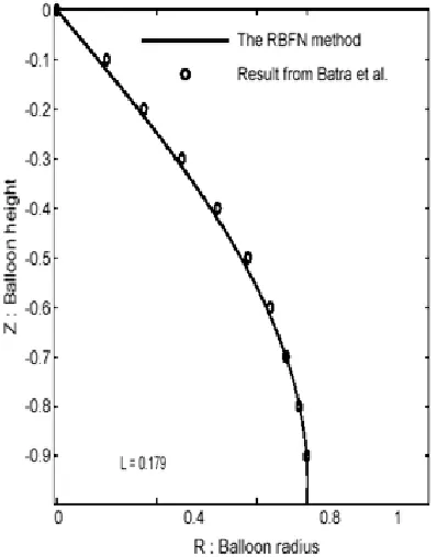
A set of 21 collocation points distributed regularly on the balloon height was employed for the present method. Figure 2 shows the profiles in the non-dimensional values of the balloon for a value of P = 0.287 and ratio L = 0.179 for the Integral RBFN method and the Runge-Kutta-Fehlberg method (Batra et al., 1989a). The difference of the two methods is quite small for these examples when the CM1 (Equation (23)) of the present method reaches 10-7.

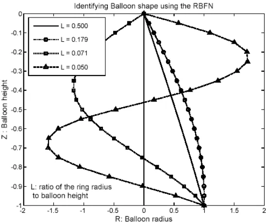
The profiles of the balloon are obtained from the Integral RBFN method for a value of P = 0.287 with a range of different ratios of the ring radius to the balloon height (L) 0.5, 0.179, 0.071, 0.05 as used by Batra et al. (1989a) are plotted in Figure 3. The results are in good agreement with those from the Runge-Kutta Fehlberg method (see Figure 5, Batra et al., 1989a) and show examples of the unstable collapsed balloon, i.e., when the yarn intersects the bobbin axis before reaching the traveller, for the smaller ratios L = 0.050 and, 0.071 while the balloon shape is stable for L = 0.5 and 0.179.

[image:8.612.206.405.288.542.2]

The convergence measurement, CM1 from Equation (23), can reach at 10-7_{, specifically 2.2x10}-7_, 4.6x10-8 and 2.6x10-8 for the three cases in Figure 3. In practice the computer time of the method was insignificant and the implementation straightforward.

[image:9.612.169.443.107.337.2]

The influence of yarn tension on the balloon profile using a range of values for P of 0.191, 0.287, 0.383, 0.40, 0.44, 0.455, at the constant ratio of ring radius to balloon height L of 0.179 is shown in Figure 4 in their real dimensions. In general, the balloon radius increases as the balloon tension decreases, i.e., increasing P. The results show that the balloon tends to collapse for the cases P = 0.44 and 0.455.

Figure 3. The profile of the yarn balloon for different ratios of the ring radius to balloon height of 0.5, 0.179, 0.071 and 0.05, ( 2 2

o o

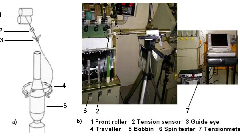
(ii) Investigating the reliability of the RBFN based predicted balloon using experimental results The analysis of the balloon shape using integral RBFN based predictions in the absence of the air drag force have been compared with experimental results obtained at CSIRO. The experiments were made using the SERMATES 82KA spin-tester machine with a 50mm inner ring diameter (Figure 5b). In order to limit the effect of the air drag force on the tension, a low angular velocity (8300 rpm or 870 radian/sec) was applied to spin 28 Tex single yarns. The balloon profiles were obtained using a high speed camera ‘Motion-Scope’ triggered by a sensor positioned close to the ring that monitored the traveller position. The traveller sensor was synchronised to a flash light to illuminate the profile of the fine yarn and this allowed individual balloon profiles to be recorded for analysis using the graphical software ImageJ.

In the analysis, the tension To was measured directly on the spin-tester during spinning by a tension-meter (Figure 5a&b). A tension sensor located between the front rollers and guide eye and the signals of balloon tension are processed at unit 7, Figure 5b. Then the tension was analysed by EDAS software and averaged over 15 seconds.

The range of the non-dimensional parameter P in which the difference of the balloon profiles between with and without air drag cases is insignificant as mentioned in Batra et al. (1989a&b) are considered in this sections. As for Figure 4, the experimental balloon profiles in this subsection (ii) are shown with their real dimensions in mm.

[image:10.612.176.440.62.318.2]

The pictures reproduced in Figures 6, 7, 8 and 9 of balloon profiles were obtained for different balloon heights and with various tensions obtained using travellers of different mass. The parameters are detailed in Table II.

In order to evaluate the accuracy of the method, a measure of the norm error of the predicted solution, Ne, is defined as

( )

( )

(

)

( )

2 n

mea i pre i i 1

e n ₂

mea i i 1

r z r z

N

r z

=

=

−

=

∑

∑

where rmea(zi) and rpre(zi) are the radius of the measured and predicted balloon shapes respectively at the position zi from the root 0 (guide eye) of balloon and n is the number of check points.

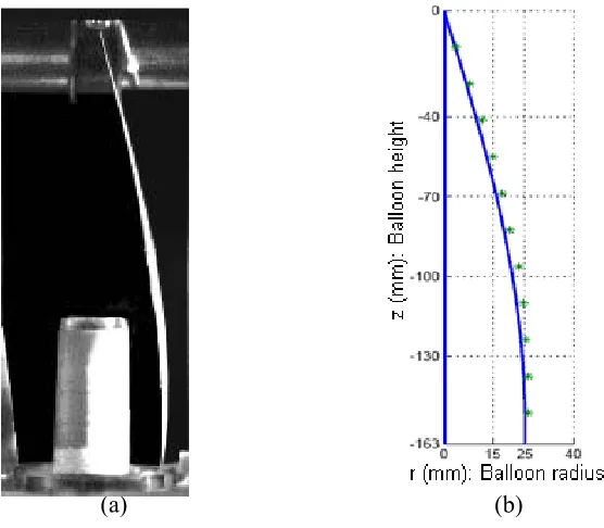
Figure 6(a) shows a balloon profile for ‘Case 1’ in Table II when the yarn is located near to the base of the bobbin. The measured tension and the balloon height are shown in Table II together with the other operating parameters for the spinning process. Figure 6(b) compares the experimental profile (* line) with the predicted shape (solid line) and Table III shows the measured and predicted values of the balloon shape which gives the associated norm error Ne of 0.082. Figures 7(a,b) and 8(a,b) show the measured shape and the predicted shape when the yarn was positioned near to the top (Case 2) and the middle (Case 3) of the bobbin, respectively.

Generally, the predicted shapes show reasonable agreement with the experimental data for balloons with a stable shape and the differences are probably linked to the influence of the air drag force in the measured data which curves and distorts the plane of the balloon. The differences between the predicted and the measured shapes increase (as shown by Ne) when the ratio of the ring radius to the balloon height decreases (c.f. Figures 6, 8(b) with Figure 7(b)) or the tension To decreases (c.f. Figure 9(b) with Figure 6(b)). In both instances the effect of the air drag force would increase.

[image:11.612.94.514.61.299.2]

Parameters Case 1 Case 2 Case 3 Case 4 Yarn linear density ρ (10-4_{g/cm) (28 Tex) 2.8 2.8 2.8 2.8}

Operating Tension To (cN) 23.4 23.0 22.4 17.0

Ring radius ro (cm) 2.5 2.5 2.5 2.5

Balloon height (cm) 25.7 16.3 20.0 28.7 Angular velocity ω (rad/s) 870 870 870 870 L = ro / h 0.097 0.153 0.125 0.087

Non-dimensional term 2 2

o o

P= ρωr / T 0.237 0.240 0.243 0.280

[image:12.612.139.474.58.235.2]

Balloon profiles are shown in Figures 6 7 8 9

Table II: Typical data for yarn and machine parameters

i zi(mm) rmea(mm) rpre(mm) i zi(mm) rmea(mm) rpre(mm) i zi(mm) rmea(mm) rpre(mm)

1 0 0 0 8 96.25 34.72 31.60 15 192.50 41.23 38.10

2 27.50 5.79 5.24 9 110.00 37.62 34.50 16 206.25 38.34 36.38 3 13.75 9.40 10.35 10 123.75 41.23 36.65 17 220.00 33.28 34.06 4 41.25 17.36 15.31 11 137.50 42.68 38.30 18 233.75 29.66 31.15 5 55.00 21.70 20.00 12 151.25 43.40 39.23 19 247.50 26.04 27.68 6 68.75 25.32 24.31 13 165.00 43.55 39.52 20 257.00 25.00 25.00 7 82.50 30.38 28.20 14 178.75 42.68 39.13

Table III. Typical data for measured (rmea) and predicted (rpre) balloon profile positions (i = 1-20) for Case 1

(a) (b)

[image:13.612.167.455.60.338.2]

(a) (b)

[image:13.612.171.449.423.666.2]

(a) (b)

[image:14.612.175.428.72.346.2]

(a) (b)

Figure 8. Case 3. (a) Balloon shape from the high speed camera; (b) Comparison of the balloon shape (solid line) from (a) and the predicted balloon shape (*). The parameters are given in Table II and the norm error Ne is 0.08.

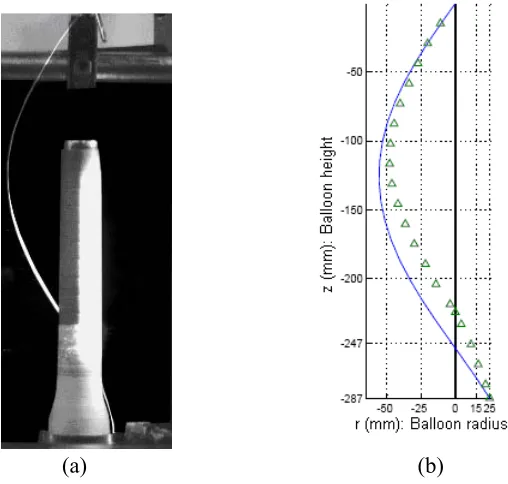
[image:14.612.188.442.416.658.2]

When the tension To was reduced by using travellers of lighter mass the profile of a collapsed balloon was obtained at the tension To = 17.0cN as shown in Figure 9 (a) with the other parameters as shown for Case 4 (Table II). The difference between the predicted shape (solid line) and the measured shape is significant (Ne = 0.2) but in this case the real shape is no longer planar and is affected where the yarn balloon touches the bobbin compared with the predicted shape which is assumed to be planar. Nevertheless the broad features of the experimental profile are shown by the theoretical curve.

5. Concluding remarks

The Integral RBFN method was used to solve the uncontrolled yarn balloon shape as described by a non-linear differential governing equation. A key feature of the method has been the solution of the non-linear equation without any of the simplifying assumptions used by previous researchers. The results show the method is reliable in determining the profile of the balloon with a simple analysis using a coarse number of collocation points, i.e., the accuracy is high with an insignificant computation time, when the balloon shape is stable. The dimensionless technique benefits the training process of the RBFN method and increases significantly the accuracy of results. This theoretical analysis compared very well with other studies by identifying the key features of ring-spinning. Comparison of the theoretical balloon profiles was consistent with the experimental balloon shapes across a wide range of spinning conditions. The differences between the theoretical and experimental data may be due to the presence of air drag and the Integral RBFN method provides a basis for further analysis allowing for the effect of air drag and time dependent effects.

Acknowledgements

Canh-Dung Tran is supported by a CSIRO Postdoctoral Research Fellowship and a grant of computing time from Australia Partnership for Advanced Computing (APAC) National Facility. The authors note the assistance of Phil Henry (TFT, CSIRO) in the preparation of the spin-tester machine SERMATES for measuring the tension and determining the profile of yarn balloons. All of this support is gratefully acknowledged.

References

Batra, S.K., Ghosh, T.K. and Zeidman, M.I., 1989a. An Integrated Approach to Dynamic Analysis of the Ring Spinning Process: Part I: Without Air Drag and Coriolis Acceleration, Text Res. J., 59, 309-317.

Batra, S.K., Ghosh, T.K. and Zeidman, M.I., 1989b. An Integrated Approach to Dynamic Analysis of the Ring Spinning Process: Part II: With Air Drag, Text. Res. J, 59, 416-424.

Behera, B.K. and Muttigi, S.B., 2004. Performance of error back propagation vis a vis Radial Basis Function Neural Network. Part I: Prediction of Properties for Design Engineering of Woven Suiting Fabrics, J. Text. Inst., 95, 284-300.

Cheng, L. and Adams, D., 1995. Yarn strength prediction using Neural Networks, Part I: Fiber properties and yarn strength relationship, Text. Res. J. 65(9), 495-500.

Clark, J.D., Fraser, W.B, Sharma, R. and Rahn, C.D., 1998. The dynamic response of a balloon yarn: Theory and experiment, Proc. R. Soc. Lond. A, 454, 2767-2789.

De Barr, A.E.., 1961. The role of air drag in Ring Spinning, J. Text. Inst. 52, T126-T139.

De Barr, A.E. and Catling, H. 1965, The principles and theory of ring spinning. Manchester, Butterworths.

Fan, J. and Hunter, L., 1998. A worsted Fabric Expert System, Part II: An Artificial Neural Network model for predicting the properties of Worsted Fabrics, Text. Res. J. 68(10), 763-771. Franke, R., 1982. Scattered data interpolation: test of some methods, Math. Comput. 48, 181-200. Fraser, W.B., 1993. On the theory of ring spinning, Phil. Trans. R. Soc. Lond. A, 342, 439-468. Fraser, W.B. and Stump, D.M., 1998. Yarn twist in the ring-spinning balloon, Proc. R. Soc. Lond. A 454, 707-723.

Hannah, M., 1952, Applications of a theory of the spinning balloon. Part I, J. Text. Inst. 43, T519-T535.

Hannah, M., 1955, Applications of a theory of the spinning balloon. Part II, J. Text. Inst. 46, T1-T16.

Hardy, R.L., 1971. Multi-quadric equations for topography and other irregular surfaces, J. Geophys. Res., 176, 1095-1915.

Haykin, S., 1999. Neural networks: A comprehensive foundation. New Jersey: Prentice Hall. He, J.H., 2004. Accurate Identification of the Shape of the Yarn Balloon, J. Text. Inst., 95, 187-191.

Kansa, E.J., 1990a. Multi-quadrics - A scattered data approximation scheme with applications to computational fluid dynamics-I: Surface approximations and partial derivatives estimates. Comput. Math. Appl., 19(8-9), 127-145.

Kansa, E.J., 1990b. Multi-quadrics - A scattered data approximation scheme with applications to computational fluid dynamics-II: Solutions to Parabolic, Hyperbolic and Elliptic Partial Differential Equations, Computers Math. Applic. 19(8-9), 147-161.

Lisini, G.G., Nerli, G. and Rissone P., 1981. Determination of balloon surface in textile machines. A finite segment approach, J. of Engineering for Industry, Transaction of the ASME, 103, 424-430. Lisini, G.G., Giusti, R., Toni, P., D. and Quilghini, D., 1994. A Mathematical model of ring spinning process, Meccanica, 29, 81-93.

Mack, C., 1953. Theoretical study of ring and cap spinning balloon curves (with and without air drag), J. Text. Inst., 44(11), T483-T497.

Mai-Duy, N. and Tran-Cong, T., 2001. Numerical solution of Navier-Stokes equations using multi-quadric radial basis function networks, Neural Networks, 14, 185-199.

Padfield, D.G., 1958. The motion and tension of an Unwinding Thread, I, Proc. R. Soc. London A, 245, 382-407.

Pynckels, F., Kiekens, P., Sette, S., Van Langenhove, P. and Impe, K., 1997. Use Neural Nets to simulate the spinning process. J. Text. Inst. 88(4), 440-447.

Sette, S. and Bouliart, L., 1996. Fault Detection and Quality Assessment in textile, Int. J. Clothing Sci. Technol., 8(1/2), 73-83.

Stump, D.M. and Fraser, W.B., 1996. Transient solutions of the ring-spinning balloon equations, J. Applied Mech. 63, 523-528.

Tran-Canh, D. and Tran-Cong T., 2002a. BEM-NN computation of Generalised Newtonian Flows, J. Eng. Anal. with Boundary Elements, 26, 15-28.

Tran-Canh, D. and Tran-Cong, T. 2002b. Computation of visco-elastic flow using Neural Networks and Stochastic Simulation, KARJ, 14(2), 161-174.

Tran-Canh, D. and Tran-Cong, T., 2004. Mesh-less simulation of dilute polymeric flows using Brownian Configuration Fields, KARJ, 16(1), 1-15.

Tran, C.D. and Phillips, D.G., 2006. Predicting Torque of worsted singles yarn using an efficient RBFN based method, J. Text. Inst., Vol. 98 (5), 387-396.

Turteltaub, M.J. and Bejar, M.A., 1976. Balloon collapse in ring spinning, J. of Engineering for Industry, Transaction of the ASME, 658-663.