Magnetohydrodynamics of Wind-Cloud Interactions: Filament Formation in the Interstellar Medium

(1)

Magnetohydrodynamics of Wind-Cloud

Interactions: Filament Formation in the

Interstellar Medium

Wladimir Eduardo Banda Barrag´an

A thesis submitted for the degree of

Doctor of Philosophy

of The Australian National University

Research School of Astronomy & Astrophysics

(2)

(3)

NOTES ON THE DIGITAL COPY

This thesis makes extensive use of the hyperlinking features of LATEX. References to

chapters, sections, subsections, figures, tables, and the literature can be navigated from within the PDF by clicking on the respective links. Internet addresses will be displayed in a browser.

(4)

(5)

(6)

(7)

Disclaimer

I hereby declare that the work in this thesis is that of the candidate alone, except where indicated below or where appropriately acknowledged in the text of the thesis. The work was undertaken between March 2012 and December 2015 at the Australian National University (ANU) in Canberra. It has not been submitted in whole or in part for any other degree at this or any other university.

This thesis is based on three manuscripts of my authorship: 1)Banda-Barragán et al.(2016), published in MNRAS;Banda-Barragán et al.(2017a), submitted to MNRAS; and 3)Banda-Barragán et al.(2017b), in preparation. These papers have been re-formatted to maintain consistency with the ANU thesis style. The chapters in this thesis contain updated and expanded information fromBanda-Barragán et al.(2016) and preliminary results fromBanda-Barragán et al.(2017a,b).

All the work presented in the above papers and the chapters of this thesis was performed solely by the candidate, who also wrote the text in its entirety. I also acknowledge helpful discussions and critical feedback provided by my supervisors, by the co-authors of my papers, as well as by the three expert examiners of this thesis. This panel of examiners and the Dean of the College of Physical and Mathematical Sciences at ANU accepted this thesis on 30th March 2016.

The original version of this thesis was submitted on 17th December 2015. This revised copy contains several improvements, additions, and minor corrections, which were suggested by the panel of examiners.

(8)

(9)

Acknowledgments

I would like to thank the academic staff at the Research School of Astronomy and Astrophysics (also known as Mount Stromlo Observatory) of The Australian National University for providing great assistance for the completion of my PhD. In particular, I thank my supervisors, Dr. Roland Crocker, Dr. Christoph Federrath, Prof. GeoffBicknell, Dr. Ross Parkin, and Dr. Ralph Sutherland for their guidance and support throughout my PhD.

Some of the analyses reported in this thesis required specific inputs from my supervisors, so I would like to thank: Dr. Roland Crocker for sharing with me first-hand information on the new findings in Galactic Centre phenomena, which I use in Chapter8; Dr. Christoph Federrath for allowing me to use his turbulence simulations as inputs for the turbulent cloud models presented in Chapter7; Dr. Ross Parkin for allowing me to modify his C code and adapt it to my data analysis needs; Prof. Geoff Bicknell for sharing his lecture notes on Astrophysical Gas Dynamics and High-Energy Astrophysics upon which some of the equations in this thesis are based; and Dr. Ralph Sutherland for allowing me to use his cloud-generating code for the fractal cloud models reported in Chapter4and for providing me with a tabulated, atomic cooling function for my calculations in Chapter8.

I also thank the Information Technology support (sysman) at both Mount Stromlo Observatory and the National Computational Infrastructure for helping me with technical advice at various stages during my studies. Additionally, I thank Prof. Mark Morris for hosting me during a visit to The University of California - Los Angeles, as well as Prof. Cornelia Lang at The University of Iowa and Prof. Naomi McClure-Griffiths at The Australian National University for insightful discussions on the potential applications of the simulations presented here.

(10)

On the technical side I would like to thank the developers of the VisIt visualisa-tion software (seeChilds et al. 2012), the Interactive Data Language (IDL,http: //www.exelisvis.com/ProductsServices/IDL.aspx), and the ’gnuplot’ graphing utility (http://www.gnuplot.info/), with which I have analysed the data obtained from my numerical work. The 2D slices, 3D plots, and movies reported in this thesis were generated using VisIt scripts, while the curves were created embedding gnuplot commands in bash scripts. This research has also made use of the SIMBAD database, operated at CDS, Strasbourg, France (seeWenger et al. 2000).

On the personal side I would like to thank my family in Ecuador (Ruth, Sheila, Vanessa, Alice, Hugo and all my relatives), my partner Helga (who kindly provided me with very helpful feedback on my thesis and papers), and all my Stromlo friends and Downer soccer fellows for their friendship and support during my PhD at Mount Stromlo.

(11)

Abstract

Filaments are ubiquitous in the interstellar medium, yet their formation, internal structure, magnetic properties, and longevity have not been analysed in detail. In this thesis I report the results from a comprehensive numerical study that investig-ates the characteristics, formation, dynamics, and global evolution of filamentary structures arising from (magneto)hydrodynamic interactions between supersonic winds and interstellar clouds. Here I improve on previous wind-cloud simulations by utilising higher numerical resolutions, sharper density contrasts, more complex magnetic field configurations, and more realistic systems with turbulent clouds. I use gas multi-tracking algorithms and state-of-the-art visualisation techniques to study the physical mechanisms acting upon wind-swept clouds. I find that material originally in the envelopes of the clouds is removed and transported downstream to form filamentary tails, while the cores of the clouds serve as footpoints and late-stage outer layers of these low-density tails. The evolution of filaments comprises four phases: 1) tail formation, 2) tail erosion, 3) footpoint dispersion, and 4) filament free floating. Overall, wind-cloud interactions produce filaments with aspect ratios & 10, lateral expansions _⇠ 1 3 of the core radius, mixing fractions _⇠

10 30%, velocity dispersions⇠0.02 0.05of the wind speed, and magnetic field

amplifications by factors of⇠10 100.

I find that the strength of magnetic fields regulates vorticity production: sinuous filamentary towers arise in non-magnetic environments, while strong magnetic fields inhibit small-scale Kelvin-Helmholtz perturbations at boundary layers mak-ing tails less turbulent. The orientation of magnetic fields also influences the morphology of filaments: magnetic field components aligned with the direction of the wind favour the formation of pressure-confined flux ropes inside the tails, whilst transverse components tend to form current sheets and favour the growth of Rayleigh-Taylor perturbations at the leading edge of the clouds.

(12)

their tails. In all models the magnetic energy enhancement saturates when the ratio of turbulent kinetic to turbulent magnetic energy densities is⇠5 10. At the end of this thesis I discuss the relevance of this work for the study of clouds and filaments in the Galactic centre and provide my perspectives on potential future research in this field. Using ray-tracing techniques I create synthetic emission maps of wind-swept clouds and compare them with radio observations of high-latitude

H clouds and non-thermal filaments in this region of the Galaxy. I interpret these structures as remains of the interplay between outflows driven by localised star formation and dense clouds in the surrounding medium. The simulated morphology, lifespan, magnetic properties, and kinematics are consistent with those inferred from observations of these clouds and non-thermal filaments.

(13)

LIST OF FIGURES

1.1 Sketch of the wind-cloud interaction problem. . . 5

3.1 Sketch of the tracers of cloud, core, and envelope material. . . 19

4.1 Simulation set-up for 2D cylindrical clouds with smoothed density profiles. . . 31

4.2 2D plots showing the time evolution of three models with uniform and fractal (adiabatic and isothermal) clouds. . . 34

4.3 Time evolution of the velocity dispersions and mixing fractions in 2D models with uniform and fractal clouds. . . 36

4.4 2D plots showing the time evolution of the plasma beta ( =Pth/Pmag, i.e., the ratio of thermal to magnetic pressure), in different 2D MHD models. . . 39

4.5 Sketch showing the transverse field effect in 2D simulations. . . 40

4.6 Evolution of the plasma beta in 2D wind-cloud models with different initial magnetic field topologies. . . 41

4.7 Comparison of the lateral elongations and mass fluxes in 2D HD models with different resolutions. . . 43

4.8 2D snapshots of model 2dHDu at different resolutions. . . 44

(18)

5.2 Density profile along the radial direction of the spherical clouds presented in this chapter. The profile is obtained from Equation (4.5) withN=10. . . 51 5.3 3D volume renderings of the logarithm of the mass density of

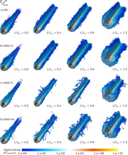
clouds/filaments in models with uniform clouds. . . 54

5.4 Density structure of the cloud and tail along the X2 direction in different models with uniform clouds. . . 55

5.5 Time evolution of the average core density, the elongation of the cloud core in theX1direction, and the mass flux of stripped material flowing through the back surface of the simulation domain. . . 56

5.6 2D slices atX3 = 0showing the logarithmic mass density in both cloud and wind material in models HD (Panel A) and MHD-Ob (Panel B). . . 58

5.7 2D slices atX1 =0of model MHD-Ob at different resolutions. . . . 64 5.8 Resolution study of some of the diagnostics used in this and

sub-sequent chapters for the study of 3D wind-cloud models. . . 66

6.1 2D slices atX3 = 0showing the evolution of the logarithm of the mass density in cloud/filament, envelope/tail, and core/footpoint material. . . 74

6.2 Time evolution of the filaments’ aspect ratios, transverse velocity dispersions, and mixing fractions. . . 76

6.3 3D volume renderings of the logarithm of the magnetic energy density of filaments in models with uniform clouds. . . 84

6.4 Time evolution of the plasma beta and the magnetic energy enhance-ment in the filaenhance-ments’ tails and footpoints.. . . 86

6.5 2D slices at X3 = 0 showing the evolution of plasma betas at 7 different times.. . . 88

6.6 Comparison of 3D volume renderings of the logarithmic mass dens-ity and magnetic energy in adiabatic ( =1.67) and quasi-isothermal

( =1.10) models. . . 93

6.7 Time evolution of the transverse velocity dispersions and elong-ations along theX1 direction of filaments in adiabatic and quasi-isothermal models. . . 94

(19)

6.8 Displacement of the centre of mass in the direction of streaming and bulk velocity of the filaments entrained in the wind. . . 96

6.9 Comparison between the time evolution of the quantities shown in Figures 6.2 and 6.7 for two models with oblique magnetic fields (MHD-Ob) at the same resolution (R64), but different domain sizes. 98 6.10 Comparison between the time evolution of the quantities shown in

Figure 6.4 for two models with oblique magnetic fields (MHD-Ob) at the same resolution (R64), but different domain sizes. . . 100 6.11 Comparison between the time evolution of the quantities shown in

Figure 6.8 for two models with oblique magnetic fields (MHD-Ob) at the same resolution (R64), but different domain sizes. . . 100

7.1 Initial density profiles of 3D uniform and turbulent clouds. . . 108

7.2 PDF of the gas density in turbulent cloud models. . . 110

7.3 3D volume renderings of the logarithm of the mass density in tur-bulent filaments.. . . 115

7.4 2D slices atX3 = 0showing the evolution of the logarithm of the mass density in different layers of the turbulent filament in model MHD-Tu. . . 117

7.5 3D renderings of the logarithm of the magnetic energy density in turbulent filaments. . . 119

7.6 3D streamline plots showing the topology of the magnetic field lines in the entire simulation domains of models MHD-Ob, MHD-Tu, and MHD-Tu-S. . . 122

7.7 Time evolution of the aspect ratios and lateral expansions of turbu-lent filaments. . . 124

7.8 Time evolution of the transverse velocity dispersions and mixing fractions in turbulent filaments. . . 125

7.9 Time evolution of the components of the energy density in turbulent filaments. . . 127

7.10 Illustration of the mechanism that leads to the saturation of magnetic energy in turbulent clouds. . . 128

(20)

7.12 3D volume renderings of the logarithm of the mass density in a model with a supersonically-turbulent cloud. . . 131

7.13 Comparison between the time evolution of the quantities shown in Figure 7.7 (Panels A1,2 and B1,2) and Figure 7.8 (Panels C1,2 and D1,2) for two models with turbulent magnetic fields (MHD-Tu-S) at the same resolution (R64), but different domain sizes. . . 133 7.14 Comparison between the time evolution of the quantities shown in

Figure 7.9 for two models with turbulent magnetic fields (MHD-Tu-S) at the same resolution (R64), but different domain sizes.. . . 134 7.15 Comparison between the time evolution of the quantities shown in

Figure 7.11 for two models with turbulent magnetic fields (MHD-Tu-S) at the same resolution (R64), but different domain sizes. . . 135

8.1 Preliminary maps at t/tcc = 0.4 of the synchrotron emission as-sociated with quasi-isothermal wind-swept clouds immersed in different magnetic fields. . . 149

8.2 Distance travelled by adiabatic (Tu-Ad) and isothermal (Tu-Is) clouds entrained in winds with different speeds. . . 153

8.3 Evolution of the bulk speed of adiabatic (Tu-Ad) and isothermal (Tu-Is) clouds entrained in winds with different speeds. . . 154

8.4 Time evolution of the line-of-sight velocity dispersions of adiabatic (Tu-Ad) and isothermal (Tu-Is) clouds entrained in a global wind of different speeds. . . 156

8.5 Preliminary syntheticHIand H↵emission maps of an isothermal wind-swept cloud. . . 159

A1.1 2D snapshots att/tcc =0.2(Panel A) andt/tcc=0.4(Panel B) of quasi-isothermal wind-cloud models with different viscosity coefficients. 200

A1.2 Same as Figure A1.1 fort/tcc =0.6(Panel C) andt/tcc=1.0(Panel D).201 A2.1 2D slices atX3 =0showing the divergence of the magnetic field in

model MHD-Tu-S at three different times: t=0,t=0.1, andt=0.4. 206

A2.2 Curves showing the cleaning process of the divergence errors in the initial magnetic fields prescribed for models MHD-Tu-W (double-dot-dashed line) and MHD-Tu-S (solid line) in Chapter 7. . . 207

(21)

LIST OF TABLES

2.1 The wind-cloud problem in the literature. . . 11

2.2 The shock-cloud problem in the literature. . . 14

4.1 Simulation parameters for different 2D models with uniform and fractal clouds. . . 32

4.2 Simulation parameters for different 2D MHD models with uniform clouds. . . 37

4.3 Simulation parameters for the 2D HD models with uniform clouds, employed in a resolution study. . . 42

5.1 Simulation parameters for different 3D models with uniform clouds. 52

5.2 Simulation parameters for the MHD models with uniform clouds employed in a 3D resolution study. . . 63

6.1 3D models of uniform clouds interacting with winds. . . 72

6.2 Growth times of the Kelvin-Helmholtz and Rayleigh-Taylor instabil-ities in different models. . . 82

7.1 Simulation parameters for different turbulent cloud models. . . 111

8.1 Initial conditions for the wind-cloud models (Ob, Tr, and Al) of the NTFs in the GC. . . 145

(22)

8.3 Initial conditions for the wind-cloud models (Tu-Ad and Tu-ls) of the high-velocityHIclouds in the GC. . . 151

(23)

CHAPTER 1 INTRODUCTION

F

are ubiquitous in the Universe. They can arise from a variety of dynamic processes occurring in both the interstellar medium (here-after ISM) and the intergalactic medium (here(here-after IGM). Shock waves, gravita-tional forces, turbulence, and magnetically-driven events can together or separately be involved in the formation of filaments (seeBiermann, Brosowski & Schmidt 1967;Schneider & Elmegreen 1979;Alfven 1981;Alfvén 1986;Rosner & Bodo 1996;

Wada, Spaans & Kim 2000;Bicknell & Li 2001a;Rodríguez-González et al. 2008;

Ntormousi et al. 2011;Pittard & Goldsmith 2016, and references therein for dis-cussions on cosmic filaments formed in different environments). In this thesis, nonetheless, I focus my analysis exclusively on filamentary structures that arise from the interplay between winds and clumps in the ISM of galaxies.

1.1. Filaments in the interstellar medium

Filamentary structures have been observed at all scales in the ISM and range from the relatively small cometary tails found in the Solar System (see e.g.,Brandt & Snow 2000;Buffington et al. 2008;Mendis & Horányi 2013), through the optical,

X-ray, and infrared filamentary shells observed in supernova remnants (see e.g.,

Hester et al. 1996;Koo et al. 2007;Shinn et al. 2009;Patnaude & Fesen 2009;Dopita et al. 2010;Vogt & Dopita 2011;McEntaffer et al. 2013;Nynka et al. 2015), the pillars and trunks in molecular complexes (see e.g.,Carlqvist, Gahm & Kristen 2003;Sahai et al. 2012a,b;Wright et al. 2012;Torii et al. 2014;Enokiya et al. 2014;

(24)

CHAPTER 1. INTRODUCTION

(see e.g.,Yusef-Zadeh, Morris & Chance 1984,Morris & Yusef-Zadeh 1985; Yusef-Zadeh et al. 1986;Bally & Yusef-Zadeh 1989,Lang et al. 1999a,LaRosa et al. 2000,

2004,Yusef-Zadeh, Hewitt & Cotton 2004,Morris, Zhao & Goss 2014), to the large-scaleH↵- andH -emitting filaments detected in star-forming galaxies (e.g.,Bland & Tully 1988; Shopbell & Bland-Hawthorn 1998; Lehnert, Heckman & Weaver 1999;Martin, Kobulnicky & Heckman 2002;Cecil, Bland-Hawthorn & Veilleux 2002;Ohyama et al. 2002;Strickland et al. 2004;Hoopes et al. 2005;Veilleux, Cecil & Bland-Hawthorn 2005for a comprehensive review; Matsubayashi et al. 2009;

Westmoquette, Smith & Gallagher 2011;McClure-Griffiths et al. 2012,2013;Bolatto et al. 2013).

Outside the Milky Way boundaries, it is also possible to observe filaments emerging when galaxies are being ram-pressure stripped as they move through the IGM in gravitationally-bound galactic aggregations (see e.g.,Conselice, Gallagher & Wyse 2001;Crawford et al. 2005;Forman et al. 2007;Yoshida et al. 2008;Canning et al. 2011;Abramson & Kenney 2014;Yoshida et al. 2012;Kenney, Abramson & Bravo-Alfaro 2015).

Despite having different sizes and being observed at various wavelengths, all of these structures are believed to share a common origin, namely the interaction of fast-moving, low-density winds with ISM inhomogeneities (i.e., clumps). Both thermal and non-thermal emissions are expected from these interactions as both are connected with the emergence of shock waves and instabilities in cosmic plasmas (see Bell 1978a,b;Draine & McKee 1993;Jones, Kang & Tregillis 1994;Mac Low et al. 1994;Bocchino et al. 2000;Bell 2004;Miceli et al. 2005;Orlando et al. 2006,

2010;Helder et al. 2012;Vink 2012for discussions on emission processes involving winds/shocks and clumps).

1.2. Filaments in simulations

On the theoretical and numerical side, filamentary structures have been predicted by and/or reported in models of supernova ejecta (e.g., Stone & Norman 1992;

Melioli, de Gouveia dal Pino & Raga 2005;Melioli et al. 2006;Orlando et al. 2005,

2006, 2008; Leão et al. 2009), H regions (e.g., Mellema et al. 2006; Mac Low et al. 2007;Mackey & Lim 2010), tidally-disrupted clouds (e.g.,Burkert et al. 2012;

Schartmann et al. 2012;Ballone et al. 2013;Schartmann et al. 2015;Ballone et al. 2016), and the Galactic centre magnetosphere (e.g.,Shore & LaRosa 1999,Dahlburg et al. 2002,Sofue, Kigure & Shibata 2005), among others.

(25)

1.3. WINDS AND CLOUDS IN THE INTERSTELLAR MEDIUM

In simulations of large-scale structures, filaments are also common features. For instance, in galactic winds and fountains (e.g.,Strickland & Stevens 2000;Melioli et al. 2008,2009;Fujita et al. 2009;Cooper et al. 2008,2009;Melioli, de Gouveia Dal Pino & Geraissate 2013), galaxy clusters (e.g.,Marcolini, Brighenti & D’Ercole 2003;

Recchi & Hensler 2007;Kronberger et al. 2008;Dursi & Pfrommer 2008;Pfrommer & Dursi 2010;Vijayaraghavan & Ricker 2015), and more specialised numerical studies of wind/shock-cloud systems (e.g.,Klein, McKee & Colella 1994,Mac Low et al. 1994;Xu & Stone 1995;Jones, Ryu & Tregillis 1996;Gregori et al. 1999,2000;

Fragile et al. 2005;Nakamura et al. 2006;Shin et al. 2008;Pittard et al. 2009;Yirak, Frank & Cunningham 2010;Pittard, Hartquist & Falle 2010; Pittard et al. 2011;

Pittard 2011;Li et al. 2013b;McCourt et al. 2015) and shock-bubble systems (e.g.,

Cowperthwaite 1989;Quirk & Karni 1996;Bagabir & Drikakis 2001;Levy et al. 2003;

Niederhaus 2007;Niederhaus et al. 2008;Ranjan et al. 2008a,b;Ranjan, Oakley & Bonazza 2011).

Further contributions and recent reviews of the literature on wind-cloud and shock-cloud interactions can be found in Section 2 ofBanda-Barragán et al.(2016) and Section 1 of Pittard & Parkin (2016), respectively. Similarly, a study of the interplay between shocks and filaments (as opposed to clouds) with different orientations with respect to the shock normal has also been recently studied by

Pittard & Goldsmith(2016);Goldsmith & Pittard(2016).

1.3. Winds and clouds in the interstellar medium

(26)

CHAPTER 1. INTRODUCTION

Typical interstellar clumps include collections of solid bodies, conglomerates of stars, or entire regions permeated with gas and/or dust clouds. Both the winds and the surrounding inhomogeneities undergo dramatic physical and chemical changes when they interact. For example, solid objects sublimate when immersed in stellar winds (e.g., Mendis & Horányi 2014), stars lose mass and magnetic energy from their outer atmospheres to a prevailing external wind (e.g., Yusef-Zadeh 2003;Ballone et al. 2013), and atomic and dense clouds are disrupted by the ram pressure exerted by outflowing material (e.g.,Bally 1986;Jones, Ryu & Tregillis 1996). Another effect that has been seen in simulations of wind-swept clouds is that they can be accelerated by the net force resulting from the momentum transfer of wind material to the cloud, which acts upon the upstream side of the cloud pushing dense material downstream (e.g.,McKee, Cowie & Ostriker 1978;Gregori et al. 2000;Marcolini et al. 2005).

On the other hand, the wind itself can also be altered during these interactions and it often evolves from purely adiabatic to radiative expansion phases (e.g.,Castor, McCray & Weaver 1975;Weaver et al. 1978;Chevalier & Clegg 1985;Cioffi, McKee & Bertschinger 1988;Hartquist, Dyson & Ruffle 2004;Reynolds 2008). The transition into a highly-efficient cooling regime occurs when lateral and reverse shocks inject additional kinetic energy into the wind and excite atomic and molecular species as a result (e.g.,Dyson & Williams 1997;Koo & Moon 1997a,b;Hartquist & Williams 1998;Draine 2011). Some significant effects observed in winds when they encounter clouds in their trajectories also include ageing, deceleration, and (de)magnetisation (see e.g.,Bregman 1980;Raymond 1984;Klein, McKee & Colella 1994;Kivelson & Russell 1995;Kwak, Shelton & Raley 2009;Al ¯uzas et al. 2014).

1.4. Investigating wind-cloud systems

The importance of studying wind-cloud systems in the context of this work lies in three main points: a) the wind-swept clouds may be distorted into tail-shaped structures (i.e., filaments) by disruptive processes and magnetohydrodynamic instabilities; b) winds encountering clumpy regions in the ISM can trigger shocks that may produce detectable thermal and non-thermal emission in these filaments; and c) advective and compressive processes combined with turbulence can radically change the topology and strength of magnetic fields and ultimately lead to the appearance of magnetohydrodynamic waves and the occurrence of highly energetic processes, such as magnetic reconnection (see e.g.,Jones et al. 1996,Miniati, Jones & Ryu 1999b;Lazarian & Vishniac 1999;Lazarian et al. 2015).

(27)

1.4. INVESTIGATING WIND-CLOUD SYSTEMS

Figure 1.1 Sketch of the wind-cloud interaction problem, in which a cosmic source launches a wind of density⇢wand velocityvwthat travels through the ambient ISM and strikes a dense cloud with certain density⇢cand magnetic fieldB, to form a filamentary structure. My thesis aims at determining the properties of these filaments in different native environments.

In this thesis I systematically investigate these three aspects in detail with the help of numerical models of wind-cloud systems in which the supersonic motion of a hot wind produces filaments as it interacts with clouds of either uniform or turbulent nature. The central part of my thesis is, therefore, to study the so-called wind-cloud interaction problem (see an illustration in Figure1.1).

The remainder of this thesis is organised as follows. In Chapter2 I review the current literature on the wind-cloud problem and contextualise the present work. In Chapter3I include a description of the numerical methods, initial and boundary conditions, time-scales, and diagnostics that I employ for the study of filaments. In Chapter4I present the results of two-dimensional simulations of cylindrical clouds in hydrodynamic and magnetohydrodynamic scenarios. In Chapter5 I discuss the cloud disruption process in models with spherical clouds. In Chapter

6 I present the results of three-dimensional simulations of spherical clouds in hydrodynamic and magnetohydrodynamic models (with uniform magnetic fields). In Chapter7I present the results of three dimensional simulations of turbulent clouds in purely hydrodynamic and magnetohydrodynamic models (with non-uniform, tangled magnetic fields).

(28)

(29)

CHAPTER 2 THE WIND-CLOUD PROBLEM

A

- constitutes an idealised scenario in which an initially static, isolated cloud or a collection of clouds interact with a wind velocity field inside the boundaries of a finite volume. An alternative approach is to consider that the wind is actually static ambient gas and the cloud is a bullet moving through it with a certain velocity, e.g., ballistically. Because of the intrinsically non-linear character of the equations describing the evolution of wind-cloud interactions, these systems can only be studied analytically in simplified cases (see the pioneering work byMcKee & Cowie 1975;McKee & Ostriker 1977), and, in general, they need to be studied with the help of numerical simulations (see e.g.,Cowie et al. 1981, who presented the first numerical work of supernova ejecta interacting with a clumpy environment).

2.1. Definitions

In purely hydrodynamic studies, where source terms (e.g., radiative cooling, thermal conduction, or gravity) are neglected, a wind-cloud system is often char-acterised by three dimensionless quantities:

1) The adiabatic index of the gas:

= cp

cv, (2.1)

(30)

CHAPTER 2. THE WIND-CLOUD PROBLEM

2) The Mach number of the wind:

Mw = |v_cw|

w , (2.2)

where_|vw|⌘vw andcw =

q Pth

⇢w are the speed and adiabatic sound speed of the

wind, respectively. 3) The density contrast:

= ⇢c

⇢w (2.3)

between the cloud, ⇢c, and wind material, ⇢w (Jones et al. 1996). Note that in

Equations (2.2) and (2.3): a) I utilise normalised quantities in code units, and b) I assume an ideal single-fluid approximation characterised by a constant polytropic index, , and a uniform mean molecular weight,µ¯.

The thermal pressure of the gas, defined as Pth, can be obtained from the gas

temperature using thermodynamic relations (i.e., the equation of state of the gas). Also, if the Mach number of the wind is much higher than unity,Klein et al.(1994) andNakamura et al.(2006) demonstrated that Mach scaling is applicable. This means that the evolution of a purely hydrodynamic wind-cloud system would solely depend upon the density contrast in high-Mach-number problems.

The above parametrisation also indicates that adiabatic simulations are scale-free and therefore independent of any absolute dimensions or primitive parameters. When additional source terms, e.g., cooling or heating, are appended to the basic hydrodynamic model, the scaling of the simulations is restricted to a one-parameter scaling (see the discussion on scaling in Section 3.2 ofSutherland & Bicknell 2007a). In such cases, however, simulations are specifically designed for a pre-defined problem, and results are generally not transferable to other situations.

In magnetohydrodynamic models, i.e., in numerical simulations where magnetic fields are incorporated, a fourth parameter is included to the above list:

4) The so-called plasma beta:

= Pth

Pmag =

Pth 1 2|B|2

, (2.4)

a dimensionless number that relates the thermal pressure,Pth, to the magnetic

pres-sure,Pmag = 1₂|B|2, in a medium, needs to be specified for the system. Sometimes,

the Alfvénic Mach number,

(31)

2.2. A REVIEW OF THE LITERATURE

MA= vw

vA = vw

|B|

p_⇢w , (2.5)

is used instead. Here,vAis the Alfvén speed in the wind. The Alfvén speed is the characteristic speed at which Alfvén waves propagate through a conducting fluid (see Chapter 3 inCowling 1976). This kind of hydromagnetic waves propagate in the direction of the magnetic field lines, i.e., along them: Bkk, and they emerge when a magnetic tension force tries to restore (straighten) a disturbed magnetic field line. This is akin to the restoring force acting on a vibrating string that has been plucked (see e.g., Figures 22.1 and 22.2 in Chapter 22 ofShu 1992). Note that in Equations (2.4) and (2.5), the factor _p1

4⇡ has been subsumed into the definition

of magnetic field. Henceforth, I apply the same normalisation for the magnetic field.

Additionally, if the magnetic field is uniformly distributed in the simulation domain (as in Chapters4-6), a set of additional parameters describing the topology of the field needs to be added as an input to the simulation set-ups. In two-dimensional models a direction angle for the magnetic field is reported. This is defined as the angle between the magnetic field vectors and the wind velocity vectors. In three-dimensional models, on the other hand, two direction angles are reported. These are defined as the angles between the magnetic field vectors and the two planes on which they are projected.

If more complex magnetic fields are implemented, e.g., tangled and turbulent magnetic fields, alternative quantities, such as the maximum field strength, the average plasma beta, or parameters associated with magnetic turbulent cascades are often used as problem descriptors. These parameters are relevant, for instance, for the simulations presented in Chapter7, in which I provide a more detailed explanation.

2.2. A review of the literature

(32)

2.2.1. Review of the wind-cloud problem

Murray et al.(1993) studied how dynamic instabilities affect pressure-bound and gravitationally-bound clouds as they move subsonically through a background gas in a two-phase medium. Jones et al.(1994) employed a two-fluid numerical model to identify particle acceleration sites in cosmic bullets and showed that they can be radio sources. Schiano, Christiansen & Knerr(1995) studied wind-accelerated, radiating clouds and found that radiation losses enhance the ablation of small-scale perturbations and prolong cloud lifetimes.

Later, Jones et al. (1996) modelled cylindrical clouds threaded by aligned and transverse magnetic fields with different Alfvénic Mach numbers and found that stretching, folding, and compression of field lines are the dominant effects for field amplification. Miniati et al.(1999b) studied the exchange of kinetic and magnetic energy in two-dimensional wind-cloud interactions and showed that the magnetic pressure at the leading edge of the cloud can exceed the wind ram pressure and become dynamically important in clouds with high density contrasts with respect to the wind.

Additionally, Gregori et al.(1999,2000) explored 3D scenarios of a single cloud immersed in a magnetised wind in which the field was oriented perpendicular to the wind velocity. They showed that the growth of dynamical instabilities at the leading edge of the cloud is increased, owing to an enhanced magnetic pressure caused by the effective trapping of field lines in surface deformations. Poludnenko, Frank & Mitran (2004) described the propagation of a radiative bullet moving hypersonically through a hot ambient gas, thus forming long and thin strings, akin to those observed in⌘-Carinae nebula (seeMeaburn et al. 1996).Raga, Steffen &

González(2005) explored the effects of photoionisation on wind-swept clouds and reported that strong ionising fields can radically reduce the fragmentation of clouds by creating an interposing layer of photo-evaporated gas around them. Later, the same authors (Raga et al. 2007) carried out a comparison study between 2.5D and 3D simulations, finding that the axisymmetric models produce an artificial condensation at the head of a wind-swept bullet, which is not seen in 3D models. Later,Pittard et al.(2005) analysed the case of non-magnetised winds interacting with multiple embedded sources of mass injection in 2D and concluded that a collection of such clouds can act as a barrier for the wind if the mass injection rate in them is higher than the wind mass flux.

Marcolini et al. (2005) showed that the inclusion of thermally-conductive gas clouds in models of super-winds is essential to reproduce the observedOVI toX

(33)

[image:33.595.115.540.263.518.2]

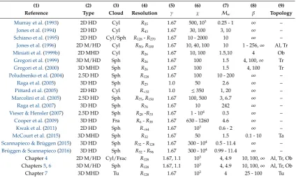
Table 2.1 Comparison between the parameter space explored by previous authors and the present work (in Chapters 4,5, and 6). Column 1 contains the references. Column 2 provides the number of dimensions considered in their simulations and whether the models reported are purely hydrodynamic (HD), magnetohydrodynamic (MHD), or both (M/HD). Column 3 indicates the type of geometry employed to describe clouds, i.e., spherical (Sph), cylindrical (Cyl), fractal (Fra), or turbulent (Tu). Column 4 indicates the resolutions (Rx) used for the simulations in terms of the number of cells (x) per cloud radius. Columns 5, 6, 7, and 8 summarise the polytropic indices ( ), density contrasts ( ), Mach numbers (Mw), and initial plasma betas ( ) reported in the references. Finally, column 9 indicates the topological structure of the magnetic field (when relevant), which could be tangled (Ta), turbulent (Tu), or aligned (Al), transverse (Tr), and oblique (Ob) with respect to the direction of the wind velocity.

(1) (2) (3) (4) (5) (6) (7) (8) (9)

Reference Type Cloud Resolution Mw Topology

Murray et al.(1993) 2D HD Cyl R25 1.67 500,103 0.25-1 1 – Jones et al.(1994) 2D HD Cyl R43 1.67 30,100 3,10 1 – Schiano et al.(1995) 2D HD Cyl/Sph R128-R270 1.67 10-2000 10 1 – Jones et al.(1996) 2D M/HD Cyl R50,R100 1.67 10,40,100 10 1-256,1 Al, Tr Miniati et al.(1999b) 2D MHD Cyl R26 1.67 10,100 1.5,10 4 Ob

Gregori et al.(1999) 3D M/HD Sph R26 1.67 100 1.5 4,100,1 Tr Gregori et al.(2000) 3D MHD Sph R26 1.67 100 1.5 4,100 Tr Poludnenko et al.(2004) 2.5D HD Sph R128 1.67 100 10-200 1 –

Raga et al.(2005) 3D HD Sph R25 1.0 50 2.6 1 –

Pittard et al.(2005) 2D HD Cyl R<32 1.0 350 1,20 1 – Marcolini et al.(2005) 2.5D HD Sph R75,R150 1.67 100,500 3,6.7 1 –

Raga et al.(2007) 3D HD Sph R76 1.67 10 242 1 –

Vieser & Hensler(2007) 2.5D HD Sph R28-R33 1.67 1-104 0.3 1 – Cooper et al.(2009) 3D HD Fra R6-R38 1.67 630-1260 4.6 1 – Kwak et al.(2011) 2D HD Sph R<64 1.67 103 0.6-2 1 – McCourt et al.(2015) 3D MHD Sph R32 1.67 50 1.5 0.1-10 Ta Scannapieco & Brüggen(2015) 3D HD Sph R32-R128 1.67 300-104 0.5-11.4 1 – Brüggen & Scannapieco(2016) 3D HD Sph R32-R96 1.67 300-104 0.99-11.4 1 –

Chapter4 2D M/HD Cyl/Frac R128 1.67,1.1 103 4,4.9 10,100,1 Al, Tr, Ob

Chapters5,6 3D M/HD Sph R128 1.67,1.1 103 4,4.9 10,100,1 Al, Tr, Ob

Chapter7 3D MHD Tu R128 1.67 103 4 25-100 Tu

ray luminosity arising from wind-swept clumps. Later,Vieser & Hensler(2007) also studied the effects of adding heat conduction to wind-swept, self-gravitating gas clouds. They found that thermal conduction can slow down the disruptive effects of instabilities arising at the wind-cloud boundaries, thus prolonging the lifetime of a cloud embedded in a hot wind. On the other hand,Brüggen & Scannapieco

(2016) showed that thermal conduction can lead to strong cloud compression by evaporation in models of multiphase galactic winds, thus opening new frontiers for further investigation on the effects of thermal conduction in wind-swept clouds.

(34)

ionisation calculations of cooling to study the hydrodynamics of high-velocity clouds (hereafter HVCs) and the processes resulting from cloud ablation, such as turbulent mixing and the production of high-velocity ions. More recently, Scan-napieco & Brüggen(2015) andBrüggen & Scannapieco(2016) presented a thorough study in 3D of the hydrodynamics of multiphase galactic outflows with cold clouds embedded in it, including radiative cooling and thermal conduction, respectively. They reported fits for the cloud disruption time-scales, cloud velocities, and the distances they travel when immersed in a wind. A resolution of64cells per cloud radius was reported as appropriate to capture the evolution of radiative clouds.

McCourt et al.(2015) performed another set of 3D simulations adding a constant magnetic field to the wind and a tangled, force-free magnetic field to the cloud. Their results suggested that an internal tangled field can suppress the disruption of the cloud and lead to fragments co-moving with their surroundings. A list of publications related to wind-cloud interactions is provided in Table2.1.

Additional publications that are relevant to the study of filaments arising from wind-cloud systems include those related to the study of shock-cloud interactions in which a shock, injected from one side of the simulation volume, impacts a cloud (or clouds) immersed in a pre-shocked medium initially at rest. The wind-cloud problem may actually be seen as a particular case of the shock-cloud problem in which the clumpy gas (i.e., a cloud) interacts with the flow behind a blast wave shock rather than with the shock itself (see Section 9 in Klein et al. 1994 for a thorough discussion).

Wind-cloud systems, however, may also be found in other scenarios in which an initial shock-driven crush is not necessarily involved, such as clouds forming and falling through thermally-unstable outflows and gaseous disks immersed in accelerating winds (see Section 5 of Schiano et al. 1995 for further details). Despite foreseeable differences in the time-scales involved in the evolution of wind-cloud and shock-cloud systems, the main aspects of the physics entailed in the cloud disruption and gas entrainment in both problems are similar. Thus, a brief summary of the literature on shock-cloud interactions is warranted. I will compare the contributions of each author with my conclusions in Section5.2, so in this section I limit myself to solely providing details of their configurations and highlights of their work.

(35)

2.2.2. Review of the shock-cloud problem

Early semi-analytical studies of shock-cloud interactions include the works by

Chevalier & Theys(1975);Woodward (1976);Nittmann et al. (1982);Heathcote & Brand(1983); andHamilton(1985). Later, the advent of novel computational algorithms and advanced tools allowed more sophisticated numerical models.

Stone & Norman(1992);Klein et al.(1994); andXu & Stone(1995), for example, described the adiabatic evolution, in 2D and 3D, of an interstellar cloud being impacted by a planar shock. Different cloud geometries and orientations were tested, but only non-radiative clouds with uniform density profiles were considered in these studies. In particular, Klein et al. (1994) showed that convergence in adiabatic HD simulations is achieved at resolutions of120cells per cloud radius. Later, Nakamura et al. (2006) introduced a mathematical function to prescribe smoothed density profiles in the clouds. Other HD simulations reported in the literature include studies of the propagation of a shock wave in the presence of multiple clouds (seePoludnenko, Frank & Blackman 2002;Melioli, de Gouveia dal Pino & Raga 2005;Al ¯uzas et al. 2012). Although less frequent than HD models, MHD simulations have also been reported in the past. Mac Low et al. (1994) introduced the first adiabatic, axisymmetric shock-cloud simulations including magnetic fields. Later,Fragile et al.(2005);Orlando et al.(2006);Shin et al.(2008);

Vaidya et al.(2013) studied the dynamic evolution of shocked clouds inserted in uniform fields in 2D, 2.5D, and 3D simulations, respectively. The formation of magnetically-dominated molecular clouds via shocks propagating through atomic clouds has also been reported in the literature (seevan Loo et al. 2007andvan Loo, Falle & Hartquist 2010).

Simulations in 2D and 2.5D have historically been used as simplifications of other-wise computationally-expensive 3D models. Nonetheless, 2D models constrain the cloud geometries and magnetic field topologies that can be employed, and this reduces the number of scenarios that can be tested computationally. For instance, turbulent flows can only be studied in 3D. More recently,Li, Frank & Blackman

(2013a,b) simulated 3D cases where the magnetic field was self-contained within the clouds, andAl ¯uzas et al.(2014) reported 2D adiabatic simulations of a shock interacting with multiple magnetised clouds.

Several shock-cloud and wind-cloud simulations reported in the literature have incorporated source terms into their mathematical description of the systems. The effects of optically-thin radiative cooling (seeMellema, Kurk & Röttgering 2002;

(36)

[image:36.595.59.481.263.552.2]

Table 2.2 Same as Table2.1, but here I present a summary of the parameter space explored in simulations of shock-cloud interactions. Column 1 contains the references. Column 2 provides the number of dimensions considered in their simulations and whether the models reported are purely hydrodynamic (HD), magnetohydrodynamic (MHD), or both (M/HD). Column 3 indicates the type of geometry employed to describe clouds, i.e., spherical (Sph), cylindrical (Cyl) or fractal (Fra). Column 4 indicates the resolutions (Rx) used for the simulations in terms of the number of cells (x) per cloud radius. Columns 5, 6, 7, and 8 summarise the polytropic indices ( ), density contrasts ( ), Mach numbers (Mw), and initial plasma betas ( ) reported in the references. Finally, column 9 indicates the topological structure of the field (when relevant), which could be tangled (Ta), turbulent (Tu), self-contained (Se); or aligned (Al), transverse (Tr), and oblique (Ob) with respect to the direction of the shock normal.

(1) (2) (3) (4) (5) (6) (7) (8) (9)

Reference Type Cloud Resolution Mw Topology

Stone & Norman(1992) 3D HD Sph R60 1.67 10 10 1 –

Klein et al.(1994) 2.5D HD Sph R60-R240 1.67,1.1 3-400 10-103 ₁ _– Mac Low et al.(1994) 2.5D MHD Cyl, Sph R25-R240 1.67 10 10-100 0.01,1 Al, Tr

Xu & Stone(1995) 3D HD Sph R11-R64 1.67 10 10 1 –

Poludnenko et al.(2002) 2D HD Cyl R32 1.67 500 10 1 –

Fragile et al.(2004) 2D HD Cyl R200 1.67 103 ₅_-₄₀ ₁ _–

Fragile et al.(2005) 2D MHD Cyl R100,R200 1.67 103 ₁₀ ₁_-₁₀₀ _{Al, Tr}

Melioli et al.(2005) 3D HD Sph R32 1.67 100,500 7 1 –

Nakamura et al.(2006) 2.5/3D HD Sph R30-R960 1.67,1.1 10,100 1.5-103 ₁ _–

Orlando et al.(2006) 2/3D HD Sph R105,R132 1.67 10 30,50 1 –

van Loo et al.(2007) 2.5D MHD Sph R640 1.67 45 1.5-5 1 Al

Orlando et al.(2008) 2.5D M/HD Sph R132-R528 1.67 10 50 1-100 Al, Tr

Shin et al.(2008) 3D MHD Sph R120 1.67 10 10 0.5-10 Al, Tr, Ob

Pittard et al.(2009) 2.5D HD Sph R16-R256 1.67 10-103 ₁₀ ₁ _–

Pittard et al.(2010) 2.5D HD Sph R128 1.67 10-103 ₁_.₅_-₁₀ ₁ _–

Yirak et al.(2010) 2.5D HD Sph R12-R1536 1.67 100 50 1 –

Pittard et al.(2011) 2.5D HD Sph R128 1.67 103 ₁_.₅_,₃ ₁ _–

Al ¯uzas et al.(2012) 2/3D HD Cyl, Sph R8-R256 1.67 10-103 ₁_.₅_-₁₀ ₁ _– Johansson & Ziegler(2013) 3D MHD Sph R100 1.67 100 30 1-103 _{Al, Tr}

Li et al.(2013b) 3D MHD Sph R54 1.67 100 10 0.25,1 Se

Al ¯uzas et al.(2014) 2D HD Cyl R32,R128 1.67 100 3 0.5-5 Al, Tr, Ob Pittard & Parkin(2016) 2.5/3D HD Sph R8-R128 1.67 10-103 ₁_.₅_-₁₀ ₁ _–

et al. 2010;Li et al. 2013b;Johansson & Ziegler 2013), thermal conduction (Marcolini et al.,2005;Orlando et al.,2006,2008;Miceli et al.,2013), photo-evaporation (Melioli et al. 2005;Tenorio-Tagle et al. 2006), and self-gravity (Fragile et al.,2004) have been considered in the past. The turbulent destruction in 2D shock-cloud interactions has also been studied byPittard et al.(2009);Pittard, Hartquist & Falle(2010); and

Pittard et al.(2011) using a non-Eulerian, sub-grid compressible turbulence model. The same model is also presented in a more recent manuscript,Pittard & Parkin

(2016), in which the authors present a resolution study for different Mach numbers and density contrasts. A list of publications related to shock-cloud interactions is provided in Table2.2.

(37)

2.3. OPEN QUESTIONS

2.3. Open questions

Notwithstanding the significant progress made towards the understanding of the processes leading to the disruption of clouds by shocks and winds in the ISM, the detailed mechanisms that lead to the formation of filamentary tails from these interactions have not been analysed thoroughly. For instance, how is the cloud disruption process associated with the formation of filaments? How do filaments evolve in time in non-magnetised and magnetised cases? How long can (magneto)tails survive against the wind ram pressure and plasma instabilities in the ISM? What is the internal structure of these filaments?

Filamentary tails have been observed in some previous simulations, but not every wind-cloud interaction has been capable of producing long-lived structures. Thus, which initial conditions really favour the formation of (magneto)tails? How does the initial magnetic field topology affect the evolution of wind-cloud interactions and the resulting tail morphology? What is the fate of the dense gas originally in the cloud cores and of their associated filamentary tails? Could high-density cores provide the required footpoints for tails to form?

There are numerical challenges involved in answering these questions, especially because of the large density contrasts that are needed. Large differences in the Courant time of wind and cloud material can make scenarios with very high density contrasts computationally expensive, so most previous studies considered cases in which the density contrasts between ambient and cloud material ranged from10 100. Realistically, however, clouds can be103 ₁₀6_{times denser than}

(38)

(39)

CHAPTER 3 METHOD

I

study the filamentary structures arising from wind-cloud interactions and provide answers to the questions discussed in Section2.3, I consider the ISM as an ideal (electrically conducting) fluid and solve the equations of fluid dynamics (simultaneously with Maxwell’s equations, in magnetised cases). In the ideal MHD approximation, which is appropriate to study astrophysical plasmas, the matter of the fluid is attached to the lines of magnetic force as if the magnetic field lines were frozen into the fluid (see e.g.,Cowling 1976). This is known as the flux-freezing theory (Alfvén 1942) and implies that the magnetic field lines move along with the fluid (a full derivation of Alfvén’s theorem is presented in

Bicknell 2012). In this chapter I describe: 1) the method and numerical solvers that I utilise to solve these systems of equations, 2) the diagnostics that I employ in subsequent chapters to analyse (2D and 3D) simulations outputs, and 3) the time-scales with which I normalise the simulation times and investigate the effects of different physical processes (e.g., turbulence) on the interactions.

3.1. Simulation code

Using the PLUTO code (seeMignone et al. 2007,2012) in either 2D,(X1,X2), or

3D,(X1,X2,X3), cartesian coordinate systems, I solve the equations of ideal

(40)

CHAPTER 3. METHOD

@⇢

@t +r·

⇥

⇢v⇤ =0, (3.1)

@⇥⇢v⇤

@t +r·

⇥

⇢vv+IP⇤ =0, (3.2)

@E

@t +r·[(E+P)v]=0, (3.3)

where ⇢ is the mass density, v is the velocity, P = Pth is the thermal pressure,

E=⇢✏+ 1₂⇢v2is the total energy density, and✏is the specific internal energy.

Similarly, in models that include magnetic fields, the relevant laws for mass, mo-mentum, energy conservation, and magnetic induction are:

@⇢

@t +r·

⇥

⇢v⇤ =0, (3.4)

@⇥⇢v⇤

@t +r·

⇥

⇢vv BB+IP⇤=0, (3.5)

@E

@t +r·[(E+P)v B(v·B)]=0, (3.6)

@B

@t r ⇥(v⇥B)=0, (3.7)

where⇢andvare defined as above,Bis the magnetic field,P=Pth+Pmag is the

total pressure (thermal plus magnetic: Pmag = 1₂|B|2),E =⇢✏+ 1₂⇢v2+ 1₂|B|2 is the

total energy density, and✏is again the specific internal energy.

To close the above system of M/HD conservation laws, I use an ideal equation of state, i.e.,

Pth =Pth(⇢,✏)= 1 ⇢✏, (3.8)

assuming a polytropic index = 5₃ for adiabatic simulations and =1.1for

quasi-isothermal simulations. In the 3D models reported in subsequent chapters, I also include additional advection equations of the form:

@⇥⇢C↵⇤

@t +r·

⇥

⇢C↵v⇤=0, (3.9)

(41)

[image:41.595.160.493.99.323.2]

3.1. SIMULATION CODE

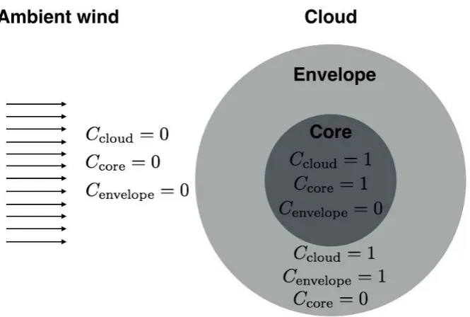
Figure 3.1 Sketch of the structure of a typical cloud in the models presented in this thesis, in which I indicate how the tracers are defined for each layer of the cloud, i.e., core and envelope. This sketch is an illustration of the gas multi-tracking technique I mention in the text, in which gas in different regions of the simulation domain are followed with additional advection equations. In subsequent chapters I explain how precisely the boundaries of these layers are defined for specific models.

whereC↵represents a set of three Lagrangian scalars used to track the evolution of gas initially contained in the cloud as a whole (↵=cloud/filament), in its core

(↵ = core/footpoint), and in its envelope (↵ = envelope/tail). Initially I define C↵ =1for the whole cloud, the cloud core, and the cloud envelope, respectively,

andC↵=0everywhere else (see Figure3.1). This configuration allows me to follow

the evolution of distinct parts of the cloud separately as they are swept up by the wind, as well as carefully examine the internal structure of the filaments that form downstream.

To solve the above system of hyperbolic conservation laws, I configure the PLUTO code to use theHLLCapproximate Riemann solver ofToro, Spruce & Speares(1994), and the (spatially unsplit) corner-transport upwind method ofColella (1990) and

Saltzman(1994) in purely hydrodynamic simulations.

(42)

CHAPTER 3. METHOD

In order to achieve the required stability (seeLax & Richtmyer 1956;Richtmyer & Morton 1967;Beckers 1992; Chapters 4 and 8 ofLeVeque 2002for discussions on the stability of numerical schemes for computational fluid dynamics), I prescribe a Courant-Friedrichs-Lewy (CFL) number (Courant, Friedrichs & Lewy,1928):

= max(|vj|+qf,j) t

n

h =0.3 (3.10)

in all cases (HD and MHD). In Equation (3.10), tn_{is the time step,} _h_⌘_min( _X j)

is the minimum cell length, |vj| are the local fluid speeds, and qf,j are the fast

(magneto)sonic speeds along each axis (j=1,2,3).

The numerical resolutions and initial conditions used in my models and char-acterised by high density contrasts and supersonic wind speeds, have not been considered in previous three-dimensional studies. Despite being adequate to de-scribe more realistic models of the ISM, the combination of these initial conditions may be challenging for some numerical solvers as a result of high-Mach-number (supersonic) flows near contact discontinuities and sharp density jumps at shocked regions (seeRyu et al. 1993,Bryan et al. 1995, andTrac & Pen 2004for detailed discussions on the high-Mach number problem in both HD and MHD simulations). In purely HD models at the locations of these supersonic flows the internal energy density,⇢✏, becomes negligible with respect to the kinetic energy density of the

gas, 1

2⇢v2, leading to significant errors when recovering the gas pressure,Pth from

the total energy,E(seeFeng et al. 2004). A similar problem occurs in MHD models with strongly magnetised media, when the magnetic energy density 1

2|B|2becomes

large compared to the other contributors, affecting the accuracy of the calculations as a result (seeTchekhovskoy et al. 2007).

These technical difficulties can be resolved in several manners. Following Feng et al.(2004), for instance, a complementary equation for the conserved entropy can be added to the system of M/HD conservation laws. This equation has the form:

@S

@t +r·(Sv)=0 (3.11)

where S = _⇢Pth1 is the modified entropy in the system. When relevant, I have,

therefore, allowed a mixed evolution of the numerical problem, in which Equation (3.11) is used to update the total energy and thermal pressure in non-shocked regions, while recovering the entropy and thermal pressure in the fully conserved way at the shock fronts.

(43)

3.2. THE CLOUD’S EQUATION OF MOTION

Alternatively, numerical diffusion can also be added to the grid cells affected by the high-Mach number problem. In order to aid code stability and mitigate the effects of the carbuncle instability (see Hanawa, Mikami & Matsumoto 2008), I have implemented small diffusion at regions of strong shocks and high magnetic pressure. This is achieved by either 1) setting floor values for the gas density and thermal pressure, 2) replacing the affected cells with predefined thresholds for the gas density and pressure, 3) averaging primitive quantities from surrounding grid cells to update those cells affected by the high-Mach-number problem, or 4) adding a small artificial viscosity to the Riemann solver fluxes with coefficient,

wk, as described byColella & Woodward 1984and implemented byParkin 2014

into the PLUTO code (I have included some examples of test simulations that incorporate different viscosity coefficients in AppendixA1).

By testing all these scenarios, I find that the combination of methods (1) and (3) produces the best and most accurate results. On the other hand, enforcing the grid cells to have floor values in method (2) leads to unphysical explosions in the simulation domain, while adding artificial viscous fluxes via method (4) probes more suitable for 2D simulations as it can make 3D runs up to_⇠1.3times more

computationally expensive than the other methods.

3.2. The cloud’s equation of motion

An important analytical result derived from the equation of momentum conser-vation (see Equation3.2) is the equation of motion of a cloud travelling through the ISM. The equation, in its simplified hydrodynamical form, can be written as follows:

mc dv_dtc

!

= 1

2CD⇢w(vw vc)2Ac, (3.12)

in the reference frame of the stationary ambient medium, wheremcandvcare the

mass and speed of the cloud,CD is the drag coefficient,⇢w andvware the density

(44)

CHAPTER 3. METHOD

Pram = 1₂⇢w(vw vc)2. (3.13)

Note that the coefficient 1

2 in front of Equations (3.12) and (3.13) is conventionally

used in the literature as it is derived from the theory of incompressible gas dynamics in accordance with the Bernoulli’s principle. However, in cases where the gas motion is supersonic, as in the study presented in this thesis, a more appropriate definition for the ram pressure would be,Pram = ⇢w(vw vc)2 (see Chapter 2 in Lunev 2009for further details).

Equation (3.12) has proved to be a useful first approximation to study the dynamics of clouds as they move through the ISM, e.g., in the surroundings of supernova remnants, where dense, pressure-confined, wind-swept inhomogeneities interact with the outer medium (see e.g.,Jones et al. 1996;Raga et al. 2007); or in the so-called galactic fountains, where ISM clouds, embedded in multiphase galactic winds, are initially advected from low to high galactic latitudes (until they reach a terminal velocity), and then they fall back onto the galactic plane as a result of the gravity. In the latter scenarios, an additional term, mcg, is added to the

right-hand side of Equation (3.12) to account for the gravitational acceleration, g, of the galaxy (see e.g.,Benjamin & Danly 1997;Zhang et al. 2015).

3.3. Diagnostics

To study the formation and evolution of filaments, a series of diagnostics, involving geometric, kinetic, and magnetic quantities, can be estimated from my simulated data. Following previous authors (Klein et al.,1994;Nakamura et al.,2006;Shin et al., 2008) I use the following global diagnostics to study the formation and evolution of filaments in my simulations:

a) The volume-averaged value of a variableF is denoted by square brackets as follows:

[_F↵]= R

FC↵dV

Vcl =

R

FC↵dV

R

C↵dV , (3.14)

whereVis the volume,C↵are the advected scalars defined in Section3.1, andVcl

is the total cloud volume. Using Equation (3.14), I define functions describing the average density,[⇢↵ ]; the average plasma beta,[ ↵ ]; the average magnetic field,

[Bj,↵ ]; and its rms along each axis,[B2_j_,↵ ].

(45)

3.3. DIAGNOSTICS

b) The mass-weighted volume average of the variableGis denoted by angle brackets as follows:

hG↵i=

R

G⇢C↵dV

Mcl =

R

G⇢C↵dV

R

⇢C↵dV . (3.15)

whereVandC↵are defined as above. Note that the total cloud volume,Vcl, and

cloud mass, Mcl in the denominators in Equations (3.14) and (3.15) are both, in

general, functions of time.

Using Equation (3.15), I define the averaged cloud extension,hXj,↵ i; its rms along

each axis,hX2

j,↵i; the averaged velocity,hvj,↵i; and its rms along each axis,hv2j,↵ i.

The subscriptj= 1,2,3specifies the direction alongX1,X2, and X3, respectively.

The initial values of the above quantities are used to normalise their averaged values and retain the scalability of the results. Velocity measurements are the exemption to this as they are normalised with respect to either the wind sound speed,cw, or the wind speed,vw.

c) Using the above definitions, I estimate the aspect ratio of filaments alongj=2,3

as follows:

⇠j,↵=

◆j,↵

◆1,↵, (3.16)

where◆j,↵are the effective radii (Klein et al. 1994) along each axis (j=1,2,3):

◆j,↵= h

5⇣hX2

j,↵i hXj,↵i2 ⌘i1

2

(3.17)

d, e) From Equation (3.17), I define the lateral expansion (alongX1) and the

displace-ment of the centre of mass of filadisplace-ments (alongX2) as◆1,↵andhX2,↵i, respectively.

f) In a similar way, I define the total (for j = 1,2,3) and transverse (for j = 1,3) velocity dispersion as follows:

v↵ ⌘| v↵|= sX

j 2

vj,↵, (3.18)

where the corresponding dispersion of thej-component of the velocity (Mac Low et al. 1994), vj,↵, reads

vj,↵ = ⇣

hv2

j,↵i hvj,↵i2 ⌘1

2

(46)

CHAPTER 3. METHOD

g) From Equation (3.19), I define the bulk velocity of filaments ashv2,↵ i. Note also

that the temporal behaviour of this parameter is used to study the acceleration of the cloud in subsequent chapters.

h) I also measure the degree of mixing between cloud and wind gas by using a mixing fraction (Xu & Stone 1995) expressed as a percentage:

fmix↵ = R

⇢C✓

↵dV

M↵,0 ⇥100 %, (3.20)

where the numerator is the mass of mixed gas, with 0.1  C✓

↵  0.9 tracking

material in mixed cells, andM↵,0represents the mass of each cloud component at

timet/tcc =0.

i) Additionally, the flux of mass through two-dimensional surfaces transverse to theX2axis is calculated from

F↵ =|F↵(Xcut)|=

Z

⇢C↵(v· ˆe2)dS ˆe2 , (3.21)

whereXcutdefines the location along the axis at which I place the reference surface,

anddSis a differential element of that surface. The surface elements are squares in this case as I am using equidistant uniform grids without mesh refinement. To maintain the scalability of the results (i.e., to work with dimensionless quantit-ies), I report the mass fluxes normalised with respect to the initial flux of wind mass through the same reference surface defined by_R Xcut, namelyFwind,0 =|Fwind,0(Xcut)|=

⇢w(vw· ˆe2)dS ˆe2.

Another set of diagnostic quantities include those related to the energetics involved in the formation of magnetotails. The enhancement of kinetic energy in cloud (filament) material is proportional to the mass-weighted velocity of the structure, so its behaviour can be studied by analysing the evolution of_hvj,↵i.

j) On the other hand, the variation of the magnetic energy contained in filament material at a specific time,t, can be studied with

EM↵ = EM↵ EM↵,0

EM↵,0 , (3.22)

where EM↵ =R 1₂|B|2C↵dVis the total magnetic energy in cloud (filament) material,

and EM↵,0 is the initial magnetic energy in the cloud.

(47)

3.4. REFERENCE TIME-SCALES

In order to quantify the kinetic energy densities in filament material, I decompose the total velocity field into mean,vj,↵ ⌘ hvj,↵i; and turbulent,v0_j_,↵, components, i.e., v↵ =v↵+v0_↵(seeKuncic & Bicknell 2004;Davidson 2004;Parkin 2014for thorough

discussions on statistical averaging in problems involving MHD turbulence). Thus, the corresponding turbulent kinetic energy density reads:

E0

k,↵ =

1

2⇢|v0↵|2. (3.23)

k) Using Equation (3.23), I define the averaged turbulent kinetic energy density of filaments as[E0

k,↵].

Similarly, to study the magnetic energy densities in filament material I decompose the total magnetic field into mean,Bj,↵ ⌘[Bj,↵ ]; and turbulent,B0_j_,↵ components,

i.e.,B_↵=B_↵+B0_↵.

l) Thus, I define the mean magnetic energy density,

Em,↵ = 1₂|B↵|2, (3.24)

and the turbulent magnetic energy density,

E0

m,↵ =

1

2|B0↵|2, (3.25)

in filament material.

m) Using Equation (3.25), I calculate the averaged turbulent magnetic energy density as[E0

m,↵]. Note that I normalise the above energy densities with respect to

the wind kinetic energy density,Ek,w= 1₂⇢wv2w.

3.4. Reference time-scales

The important dynamical time-scales in the simulations presented here are: a) The cloud-crushing time (Jones et al. 1994,1996),

tcc = 2_vrc

s =

⇢c

⇢w

!1 2 ₂_r

c

Mwcw =

1 2 2rc

Mwcw, (3.26)

wherevs = Mwcw 12 is the approximate speed of the internal shock travelling

(48)

CHAPTER 3. METHOD

shock speed is obtained by equating the post-shock pressure in the wind,⇢wv2w,

and the pressure in the shocked cloud material,⇢cv2s, i.e., from momentum flux

conservation (seeBychkov & Pikelner 1975;McKee & Cowie 1975). It is assumed that the wind is supersonic (i.e., Mw>1). Klein et al. (1994) provided a more

accurate expression for the shock speed (see Equation (5.4) in Section 5 of their paper).

In order to maintain scalability (i.e., to provide the results in dimensionless quant-ities), all the time-scales reported in this paper are normalised with respect to the cloud-crushing time.

b) The simulation time, which in this case is:

tsim =1.225tcc. (3.27)

c) The wind-passage time:

twp = 2_vrc

w =

1

2 tcc=0.032tcc. (3.28)

d) The turbulence-crossing time:

ttu = _v2rc cloud =

2rc

Mtuccloud. (3.29)

To ensure that sequential snapshots adequately capture details of the evolution of filamentary tails, simulation outputs are written at intervals of t=8.2⇥10 3_t

cc. In

reference to time resolution, our simulations are sensitive to changes occurring on time-scales of the order of2.5⇥10 5_t

cc. Other time-scales could also be defined for

wind-cloud systems, e.g., the cooling time-scale in models with radiative cooling, the free-fall time in simulations with self-gravity, and the ablation time-scale when heat conduction is included (seeFragile et al. 2004).

3.5. Computational requirements

The numerical methods described in this chapter necessitate high-performance computing. PLUTO is a portable code that works on multiple-processor architec-tures by performing parallel domain decompositions with MPI (Message Passing Interface) programming (seeMignone et al. 2012,2015and references therein for a full description of the code).