This is a repository copy of
Non-Trading, lexicographic and inconsistent behaviour in
stated choice data
.
White Rose Research Online URL for this paper:
http://eprints.whiterose.ac.uk/43612/
Article:
Hess, S, Rose, JM and Polak, JW (2010) Non-Trading, lexicographic and inconsistent
behaviour in stated choice data. Transportation research Part D, 15 (7). 405 - 417 . ISSN
1361-9209
https://doi.org/10.1016/j.trd.2010.04.008
Reuse See Attached
Takedown
If you consider content in White Rose Research Online to be in breach of UK law, please notify us by
Non-trading, lexicographic and inconsistent behaviour
in stated choice data
Stephane Hess∗ John M. Rose† John Polak‡ November 5, 2008
Abstract
This paper discusses a number of issues relating to the pre-analysis and cleaning of stated choice data, where we look specifically at the problems caused by non-trading, lexicographic and inconsistent response patterns. We argue that this process is in fact considerably more complex and challeng-ing than many in the field have hitherto acknowledged, with the standard practice being the use of of rather ad-hoc procedures for the identification of the above listed phenomena. A detailed analysis on four different stated choice datasets highlights the potential impacts of these methods on model estimation results.
1
Introduction
Econometric structures belonging to the family of random utility models (RUM) are used to provide guidance to policy makers across a range of different areas in the field of transport research. These can range from standard cost-benefit analyses of proposed infrastructure developments to social inclusion studies and evaluations looking at environmental impacts, e.g. the valuation of noise and pol-lution reductions. With this reliance on valuation outputs from choice modelling analyses, any bias in these outputs can have significant monetary, societal and environmental impacts. This in turn leads to a need to attempt to improve the robustness of the outputs of such studies.
Two main sources exist for potential bias in the outputs from choice models; misspecification of the models and problems with the data. The former includes
∗Centre for Transport Studies, Imperial College London, [email protected] †Institute of Transport and Logistics Studies, The University of Sydney, [email protected]
‡Centre for Transport Studies, Imperial College London, [email protected]
both the choice of a model structure (e.g. Nested Logit, Multinomial Logit, etc.) as well as the specification of the observed utility function. In the present paper, we are more concerned with the issue of data problems, although this can, as we will see, also have implications at the model specification end.
The vast majority of choice modelling applications reported within the liter-ature are now estimated on Stated choice (SC) data, including but not limited to the field of transport research. Although concerns do exists as to the response quality in SC data (e.g.Fujii and Garling,2003;Garlinget al.,1998;Verplanken and Aarts, 1999), SC data have significant advantages over Revealed Preference (RP) data in terms of the quality of the information describing choice situations, where measurement error and issues of alternative availability do not arise. Fur-thermore, by design, SC surveys encourage trading off between attributes, which can facilitate the calculation of willingness to pay indicators when compared to RP data, where as an example, time and cost attributes are often strongly cor-related. Finally, with SC data, analysts generally have at their disposal multiple observations for each respondent, which can for example be useful in recovering inter-respondent taste heterogeneity1
.
Having multiple observations for each individual does however have another advantage in that it provides analysts with a greater ability to investigate how the decision makers respond to varying choice situations. One interesting recent body of work in this context looks at how respondents process the information presented to them, for example allowing for the fact that some of the respondents may ignore some of the attributes that they are faced with (cf. Hensher, 2007;
Puckett and Hensher, 2007). Such approaches rely heavily on having multiple choice observations per respondent.
Allowing for differences in information processing strategies (IPS) acknowl-edges the fact that, at least within the context of the survey at hand, different respondents will process the information presented to them differently. The reser-vation of limiting this to the survey at hand is important. Indeed, while it is con-ceivable that some respondents will ignore a given attribute within a SC survey (e.g., a given respondent may ignore a road toll attribute across all eight choice situations they are presented with as part of an SC experiment), this does not imply that they are insensitive to road tolls in general. Indeed, the very nature of SC experiments which are designed to encourage attribute trading requires that the levels of each attribute present within the experiment be such that trading
1
should take place. Thus, if the levels of an attribute (toll cost in the previous ex-ample) are such that when combined with other attributes in the experiment they do not reach some psychological threshold for individual respondents, then that attribute may be ignored or not considered over the course of that experiment.
In this paper, we address three issues that fall into the broad spectrum of IPS. In particular, we investigate the prevalence of non-trading, lexicographic and (what we term) inconsistent behaviour across choice situations. While the discussion of these issues is not new (cf. Section 2), there seems to be a lack of insight into the effects of these three phenomena, and an absence of guidance on how they should be dealt with in practical modelling. This is worrying, given the high reliance on SC data in policy related studies. The present paper aims to address this issue with help of evidence from four separate SC datasets.
The remainder of this paper is organised as follows. Section 2 discusses the three modelling issues in more detail. This is followed in Section3by the results of the various empirical analyses. Finally, Section 4 presents the conclusions of the research.
2
Modelling issues
In this section, we look in detail at the three phenomena that represent the topics of interest of the present paper.
2.1 Non-trading
Non-trading in choice behaviour refers to the situation where a respondent always chooses the same alternative across choice sets.
Non-trading is a phenomenon that arises especially in the case of labelled
choice situations. As an example, in the case of a mode choice experiment, a respondent might always be observed to choose the same mode of transport, say car. Non-trading in the case of mode choice experiments often means that re-spondents stay with their current mode of transport, i.e., the non-trading extends beyond the SC framework to incorporate the chosen mode in a real-world set-ting. Another example of labelled choice experiments where non-trading can be prevalent is the choice between tolled and untolled routes.
Finally, many SC surveys include as an alternative a reference alternative in the choice situation which corresponds (either closely or fully) to a recent behavioural outcome (e.g., a recent trip that was made; see Train and Wilson 2007for a review of such experiments). In the presence of a reference alternative, non-trading has tended to be exhibited in the form of respondents always selecting their recent experience over all other options presented to them.
Non-trading is far less common in the context ofunlabelledchoice experiments (as opposed to labelled choice experiments). Nevertheless, for whatever reason (fatigue, a misunderstanding of how the experiment works, etc.) some respon-dents may still be observed to always choose a particular alternative (often the first, a result of reading the information presented to them in SC experiments from left to right).
A number of alternative explanations exist for non-trading of the form dis-cussed here. These explanations can be considered under three broad headings. The first is that non-trading may reflect the presence of extreme preference. Un-der this scenario, non-trading individuals are assumed to be responding as utility maximising agents but to possess very strong preferences for a particular alterna-tive. For example, in the case of mode choice experiments, high mode allegiance and inertia can make a respondent very unlikely to switch from their currently chosen mode. In such circumstances the SC design may not be able to offer the respondent sufficiently attractive alternatives to their preferred mode
A second and quite distinct explanation for non-trading behaviour is that it reflects a form of heuristic (i.e., non-utility maximising) decision making by the respondent, arising from misunderstanding, boredom or fatigue during the SC exercise. For example, a respondent who has lost interest in the experiment may cease to seriously consider the characteristics of the alternatives presented and instead respond mechanically with the same choice in order to hasten the end of the experiment. In less extreme cases, individuals may filter some of the attributes or alternatives presented to them in order to simplify their decision making task.
The third explanation for non-trading behaviour is that it reflects a form of political or strategic behaviour which can express itself especially in the case of controversial topics such as the building of new road tolls (see e.g. Kuriyama 2005). In this case for example, some respondents may be so opposed to the principle of road tolls that they will never choose a tolled alternative in an SC experiment, no matter how large the time savings may be. This can be aggravated in the case of respondents who believe that through expressing their preferences in this way they might be able to influence policy decisions.
quantities such as willingness to pay).
It is therefore desirable to be able to diagnose which type of non-trading be-haviour is arising. However, in the absence of additional post mortem information from the respondent on their conduct of the SC exercise, it is generally impossible to discriminate between the different regimes of non-trading behaviour.
In these circumstances it is clearly desirable to reduce the incidence of non-trading by careful design of the SC exercise, for example by reducing task com-plexity to avoid fatigue, by presenting respondents with large enough incentives to encourage them to trade between alternatives, by avoiding (where possible) the use of choice contexts that might inflame policy or political sensitivities. However, there are limitations to what can be achieved in terms of SC design alone. For example, when considering incentives it is generally not known a priori where the individual-specific thresholds lie, such that relatively large incentives may be re-quired. Moreover, presenting incentives that are too large will reduce the realism of the experiment which may again have an impact on stated choice behaviour (see e.g. Mehta et al. 1992).
Before proceeding to the issue of lexicographic behaviour, it is worth briefly highlighting the potential impacts of non-trading behaviour on model estimates in the case where the modelling framework is not designed with a view to the inclusion of such respondents. To a large extent, non-trading behaviour will impact mainly on alternative specific constants and inertia terms (if included). However, there is a possibility of some impact on marginal utility coefficients, and willingness to pay indicators by extension. This arises whenever the model is not able toexplain all of the non-trading on the basis of constants, in which case the estimation will attempt to link some of this behaviour to values of explanatory attributes. In the most extreme cases, such as when toll-averse respondents consistently reject a faster albeit more expensive option, this can seriously bias the estimates of important coefficients.
2.2 Lexicographic behaviour
The second issue addressed within this paper is that of lexicographic behaviour. Lexicographic behaviour refers to the case where over the course of the experi-ment, a respondent evaluates the alternatives on the basis of a subset of attributes (see e.g.,Blumeet al.2006;Campbellet al.2006;Deshazo and Fermo 2002; Fos-ter and Mourato 2002;Rekola 2003;Rosenbergeret al. 2003;Sælensminde 2001,
2002; Spash 2000). Common examples include respondents who always choose the cheapest alternative irrespective of the other attributes shown, or respondents who always choose the fastest alternative.
As with non-trading behaviour, lexicographic responses can arise for a number
of reasons, reflecting both genuine decision making processes or artefacts of the SC exercise. True lexicographic behaviour is difficult to detect except in the most basic of experiments. Indeed, in an experiment using only two attributes, such and time or cost, a respondent who always chooses the cheapest or fastest alternative can be easily detected to have undertaken lexicographic behaviour. Even here however, it must be stressed that the lexicographic behaviour may be constrained to the choice situations at hand, as discussed below. Difficulties arise in the case of more complex experiments, i.e., experiments involving more than just two attributes. As such, a respondent might be observed to always choose the cheapest alternative without necessarily behaving in a truly lexicographic manner, or may engage in lexicographical behaviour across subsets of alternatives which may be very difficult to detect. Indeed, it might be the case that an alternative that is more expensive has other disadvantages, for example in the form of lower frequency. Here, the design of the survey can play an important role. Furthermore, two alternatives might be equally cheap in which case a respondent might still be trading off between other attributes.
Just as with non-trading behaviour, the presence of individual-specific thresh-olds potentially plays an important role. As such, an individual will always choose the cheapest alternative unless a more expensive alternative provides savings of a sufficient magnitude along some other dimension. If this threshold is never achieved, then this respondent will likely behave in a lexicographic fashion.
The effects of lexicographic behaviour on model estimates is most easily illus-trated on the basis of a binomial design with two attributes, time and cost. Let
T Ti,t andT Ci,t represent the travel time and travel cost for alternativeiin choice
situationt, where, by design, one alternative is cheaper and one is faster. With ∆T Tt =|T T1,t−T T2,t|and ∆T Ct =|T C1,t−T C2,t|giving the absolute differences
in travel time and travel cost between the two alternatives, we have a boundary value of travel time savings (VTTS) vt =
∆T Ct
∆T Tt. Working on the assumption of
independence between the observed and unobserved utility components, we then know that a respondent choosing the cheaper of the two alternatives has a VTTS bounded above byvt, while a respondent choosing the more expensive of the two
alternatives has a VTTS bounded below byvt. We can then construct two sets
of values, vA and vR, containing the accepted and rejected VTTS respectively,
where vASvR = v with v=hv1, . . . , vTi, and with T giving the total number
of choice situations. After observing all T choices for a given respondentn, we can assume that max (vA) ≤ vn ≤ minvR, i.e., the VTTS of respondent n is
bounded below by the highest accepted VTTS and above by the lowest rejected VTTS.
the cheapest of the two alternatives, then vA = ∅, and vR = v. As such,
we can only assume that vn ≤ min (v), i.e., the value of time for respondent n is lower than the smallest boundary value of time calculated across the T
choice situations. Similarly, for a respondent who always chooses the fastest alternative, we may only know thatvn≥max (v). This means that respondents
who behave lexicographically (on one attribute) only provide us with a boundary in one direction. In turn, this means that the upper boundary for respondents who always choose the fastest alternative will potentially be overestimated, while the lower boundary for respondents always choosing the cheapest alternative will be underestimated. The relative size of these two groups in the sample population can be assumed to influence the direction of the bias, with the overall size determining the general ability of the model to estimate boundaries.
As with non-trading, the incidence of lexicographic behaviour can be reduced by offering sufficient incentives for respondents to trade off individual attributes against each other. As such, staying with the simple example above, a wide enough array of boundary VTTS should be presented to respondents. However, the aim is also to obtain a narrow interval (lower and upper boundary), such that the presented array should not be too wide.
In the case of more complex designs, it is not generally possible to distinguish between true lexicographic and apparent lexicographic behaviour. The incidence of either can however again be minimised by using designs that actively encourage trading off between attributes.
Finally, it should be said that there are instances where lexicographic be-haviour and non-trading bebe-haviour can be equivalent. One example is the case where respondents are given a choice between their current untolled option and a tolled alternative. Here, respondents who always choose their current alternative can be seen as being non-traders while also behaving in a lexicographic fashion.
2.3 Inconsistent behaviour
While the phenomena of non-trading and lexicographic behaviour have been dis-cussed extensively within the existing literature, an issue that has received some-what less exposure is some-what may be termed as inconsistent behaviour (for some examples see Sælensminde 2001). By inconsistent behaviour, we refer to situa-tions in which responses appear to violate one or more of the axioms of rational choice behaviour.
As an example of inconsistent behaviour, we may think of a choice situation where a respondent is not willing to accept the increase in cost ∆C,1 for an
alternative that is an improvement along all other dimensions by a quantity ∆O,1, where this may be a combined improvement across various attributes. If
the same respondent is later on observed to accept an improvement ∆O,2 with
∆O,2 ≤∆O,1 but ∆C,2 ≥∆C,1, then this respondent’s behaviour may be termed
to be inconsistent. Similarly, if a respondent is observed to accept the initial improvement, but then rejects ∆O,2 ≥ ∆O,1 with ∆C,2 ≤ ∆C,1, then this may
similarly be regarded as inconsistent behaviour.
Responses such as these clearly raise concerns regarding the internal validity of the SC data, especially when such data are typically analysed using models that assume rational decision making on the part of agents. However, it is impor-tant to recognise that when we are working within a random utility maxmising framework, certain forms of apparent inconsistency will be inevitable.
The effects of such inconsistent behaviour on model results is more difficult to quantify. However, one possible impact is clearly on the error associated with individual coefficients. In the presence of inconsistent behaviour, it can be expected that the stability of the estimation of concerned coefficients is reduced, potentially substantially so. In other words, the relative weight of the unobserved part of utility can be expected to increase.
At this point, it should also be noted that in some cases, apparent inconsistent behaviour can be explained on the basis of other phenomena such as reference de-pendence (cf.de Borger and Fosgerau,2007;Hess et al.,2008). This would mean that a departure from a standard linear modelling approach would be required to explain these inconsistencies.
2.4 Discussion
The above discussion has highlighted three potential phenomena that might play a substantial role in how individuals behave in the context of SC survey tasks. Clearly, to a large extent, the incidence of these three issues depends heavily on the design used in the generation of the survey questionnaires, and fewer problems might be expected with better designs. On the other hand, it should also be said that more complex designs might actually increase the incidence of lexicographic and inconsistent behaviour, in that respondents simplify the choice processes or struggle with absorbing all information, thus potentially exhibiting what may look like inconsistent behaviour.
Another factor that potentially affects the incidence of the three phenomena is the number of choice situations (and possibly also alternatives) that respondents are presented with. Indeed, with fewer choice situations, the risk of non-trading and lexicographic behaviour clearly increases. On the other hand, with a higher number of choice situations, the risk of inconsistent behaviour rises, for example due to fatigue or boredom.
poten-tially play a role and have significant impacts on model results. The incidence of any of the phenomena might be reduced by being careful at the design stage of the survey experiments. However, even with the best designs, some of the prob-lems may remain. Furthermore, a large number of studies are routinely carried out on data that was collected on the basis of less carefully designed surveys. As such, the question arises as to what should be done in the face of significant levels of non-trading, lexicographic or inconsistent choice behaviour.
Three possible approaches arise. The first is to treat the data as is, i.e., proceeding with the estimation regardless of the presence of respondents whose behaviour exhibits one of the three phenomena discussed above. The disadvan-tage of this approach is that it runs a substantial risk of including in the analysis data that were generated by decision processes (e.g., heuristics) that are quite different from those embodied in the models used to analyse the data (which typically assume (random) utility maximising behaviour). This approach thus exposes modellers to potentially significant mis-specification bias in their results. The second approach would be to remove all such respondents from the data and estimate models only on the subset of the data that is unaffected by any of the three phenomena. This however also poses problems. First, as we have discussed above, it is quite possible for circumstances to arise in which (random) utility maximising behaviour can give rise to data that appear to be contaminated by heuristic non-trading, lexicographic or inconsistent response patterns. An overly aggressive approach to data cleaning risks discarding data that are in fact valid, effectively resulting in a form of endogenous sub-sampling based on expressed preferences, which may in turn lead to biases in the estimation of tastes. Secondly, since many SC datasets contain quite high levels of (apparent) non-trading, lexicographic and inconsistent choice behaviour, an aggressive approach to data cleaning will often reduce sample size significantly and may also affect the representativeness of the estimation sample.
The third and clearly the most desirable approach is to develop the diagnostic capability to be able to discriminate between response data that are consistent with the model being applied to their analysis (typically but nor necessarily a ran-dom utility model) and those that are not. Data that are classified as consistent with the analysis model are then included and those that are not are excluded. It must be stressed that we are not arguing that data that are inconsistent with a given analysis model are of no interest. On the contrary, understanding patterns of violation is potentially extremely important in motivating the development of the underlying theory upon which analysis models are based. Our argument is simply that when we can demonstrate, with reasonable confidence, that a certain set of responses are inconsistent with a given analysis model, it makes no sense whatsoever to use this model to analyse these data.
The key issue is therefore the quality of our diagnostic capability in respect to discriminating between different regimes of response in SC experiments. Un-fortunately, at present this capability is at best rudimentary and therefore there is considerable interest in enhancing our understanding at an empirical level of the impact of different data cleaning strategies on model estimation results. This provides the motivation for the remainder of this paper.
3
Empirical studies
This section presents the findings from four separate empirical studies looking at the incidence of the three phenomena discussed in Section2.
Given the context of the present study, only simplistic Multinomial Logit (MNL) models were used in the analysis, and all models were based on a linear-in-parameters specification of the utility function. BIOGEME was used for all model estimations (cfBierlaire,2003).
3.1 Danish study
The first analysis makes use of the data collected for the DATIV study carried out in Denmark in 2004 (cf.Burge and Rohr,2004). For this survey, a binomial unlabelled route choice experiment was used, with two attributes, travel time and travel cost describing the alternatives.
Each respondent was presented with 9 choice situations, where choice situa-tion 6 contained a dominant alternative. Any respondent failing this dominance check was excluded from the data, while, for the remaining respondents, the dom-inated choice situation was removed from the estimation data. The final sample available for estimation contains 17,020 observations collected from 2,197 re-spondents.
3.1.1 Data analysis and empirical framework
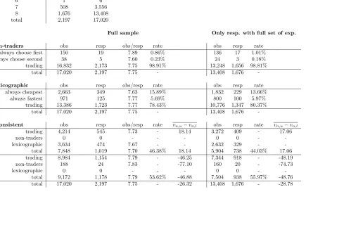
A detailed summary of the choices observed in the DATIV data is presented in Table1.
Table 1: Descriptive analysis of DATIV data
Number of choice sets Respondents Observations
3 3 9
4 4 16
5 5 25
6 1 6
7 508 3,556
8 1,676 13,408
total 2,197 17,020
Full sample Only resp. with full set of exp.
Non-traders obs resp obs/resp rate obs resp rate
always choose first 150 19 7.89 0.86% 136 17 1.01%
always choose second 38 5 7.60 0.23% 24 3 0.18%
trading 16,832 2,173 7.75 98.91% 13,248 1,656 98.81%
total 17,020 2,197 7.75 - 13,408 1,676
-Lexicographic obs resp obs/resp rate obs resp rate
always cheapest 2,663 349 7.63 15.89% 1,832 229 13.66%
always fastest 971 125 7.77 5.69% 800 100 5.97%
trading 13,386 1,723 7.77 78.43% 10,776 1,347 80.37%
total 17,020 2,197 7.75 - 13,408 1,676
-Inconsistent obs resp obs/resp rate vn,u−vn,l obs resp rate vn,u−vn,l
trading 4,214 545 7.73 - 18.14 3,272 409 - 17.06
non-traders 0 0 - - - 0 0 -
-lexicographic 3,634 474 7.67 - - 2,632 329 -
-consist. total 7,848 1,019 7.70 46.38% 18.14 5,904 738 44.03% 17.06
trading 8,984 1,154 7.79 - -46.25 7,344 918 - -48.19
non-traders 188 24 7.83 - -77.10 160 20 - -74.73
lexicographic 0 0 - - - 0 0 -
-inconsist. total 9,172 1,178 7.79 53.62% -46.88 7,504 938 55.97% -48.76
total 17,020 2,197 7.75 - -26.32 13,408 1,676 - -28.78
Another issue that was investigated was whether the placing of the dominance check in the sixth choice situation potentially has an impact on behaviour in the remaining three choice situations. Indeed, some respondents may feel patronised by being asked such asimple question and may change their behaviour thereafter. Turning to the three issues that are the topic of the present paper, we can first see that non-trading only plays a very minor role in the present dataset, with just over one percent of respondents always choosing the same alternative. Such a low rate was to be expected in the context of an unlabelled route choice experiment.
However, moving on to lexicographic behaviour, we find that a significant share of respondents consistently choose the cheapest alternative, namely 15.89% in the full sample, and 13.66% in the sample for respondents who completed a full set of choice experiments. Similarly, 5.69% (respectively 5.97%) of respondents always choose the faster of the two alternatives. This means that it is in these two groups only possible to estimate either an upper boundvn,lor a lower bound vn,u on the VTTS. The uneven sizes of the two groups mean that the overall
estimate is potentially biased downwards.
The final observation from Table 1 relates to the incidence of what we term inconsistent behaviour, where in this case, we are looking for respondents who have values invA that are larger than values in vR, i.e. respondents who accept
a higher boundary VTTS at some point only to reject a lower one later, or vice versa. As could have been expected, anyone who is a non-trader also behaves inconsistently, where this is a direct result of the variations in attributes in the design. Similarly, a respondent who behaves lexicographically cannot by defini-tion be behaving inconsistently, as either vA = ∅ or vR = ∅. This leaves us
with 1,699 respondents who are neither non-traders nor behave lexicographically (respectively 1,327 with a full set of choices). Rather worryingly, of these, only 32.01% behave consistently (or 30.82% in the reduced sample), meaning that out of all respondents, 53.62% have at least one value invA that is higher than the
lowest value invR (respectively 55.97% in the reduced sample).
Clearly, some inconsistent behaviour may be explained by small errors made by the respondents, such that occasionally, a value invA may be slightly higher
than a value invR. This is especially likely when working with complex designs
where respondents are faced with a large number of choice situations, alterna-tives and attributes. However, here, we are dealing with the most simplistic of designs, where respondents face two alternatives with two attributes, and the experiment only contains 8 choice situations. This should significantly reduce the scope for such errors. To give a further account of the level of inconsistent behaviour in the data, we calculated the difference betweenvn,uandvn,l for each
calcula-tion is only possible for respondents wherevR and vA both contain at least one
value. Here, we can see that we obtain a gap of 18.14DKK/hour2
for respondents withconsistent behaviour, while the figure for respondents withinconsistent be-haviour is−46.88DKK/hour. Similar observations are made in the subsample of respondents with a full set of choice situations. This gives a strong indication of inconsistent behaviour by respondents across choice situations.
A large number of different models were estimated recognising the various issues discussed above. In each case, a simple linear-in-parameters specification of the MNL model was used, with an additional constant for the first alternative. It could be argued that the MNL model is not the most appropriate model for this data, given recent results using non-parametric specifications byFosgerau(2006) on the same data. However, the MNL model remains the base specification in choice modelling, and it is not clear how the effects of the above three issues should play a lesser role in more advanced models.
3.1.2 Results
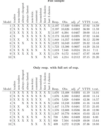
The estimation results for the DATIV data are summarised in Table2. In total, 20 different models were estimated, split into two groups of 10 models depending on whether respondents without a full set of choice situations were included or not.
The first observation that can be made from Table 2 is the relatively poor model performance in terms of the adjusted ρ2 measure. A closer inspection on simulation runs showed that the differences in utility were very small between the two alternatives, leading to very similar choice probabilities. This can potentially explain some of the observations from Section 3.1.1. If respondents struggle to differentiate between the two alternatives, then this will clearly increase the risk of lexicographic or inconsistent behaviour.
Looking next at the differences between the two sets of models, we can observe slightly better model fit for the models using the full data, while on average, the VTTS findings from the two groups of models are very similar. The remainder of this discussion will focus on the first group of models.
Here, we can firstly observe that the model fit obtained for the final three choice situations is higher than for the choice situations prior to respondents being presented with the dominated choice situation, while the VTTS is also higher, by 6%. This is not necessarily related to the positioning of the dominance check, where the better fit could for example be down to more rational choice behaviour which could be linked to learning effects.
2
Danish Kronas per hour.
Table 2: Estimation results on DATIV data (WTP indicators in DKK/hr)
Full sample
Model traders non-traders alw
ays cheap est alw ays fastest non-lexic. consisten t inconsisten t first 5 choices last 3 choices
Resp. Obs. adj. ρ2 VTTS t-rat.
1 X X X X X X X X X 2,197 17,020 0.0394 37.92 14.59 2 X X X X X X X X 2,197 10,626 0.0382 36.90 11.59 3 X X X X X X X X 2,197 6,394 0.0467 39.00 15.14 4 X X X X X X X X 2,173 16,832 0.0395 37.92 14.66 5 X X X X X X X X 1,848 14,357 0.0468 56.12 22.99 6 X X X X X X X X 2,072 16,049 0.0597 28.32 13.43 7 X X X X X X X 1,723 13,386 0.0607 44.20 24.34 8 X X X X X X X X 1,019 7,848 0.0524 28.14 7.11 9 X X X X X X X X 1,178 9,172 0.0417 47.97 16.89 10 X X X X X 545 4,214 0.2112 37.15 21.20
Only resp. with full set of exp.
Model traders non-traders alw
ays cheap est alw ays fastest non-lexic. consisten t inconsisten t first 5 choices last 3 choices
Resp. Obs. adj. ρ2 VTTS t-rat.
1 X X X X X X X X X 1,676 13,408 0.0393 41.19 14.01 2 X X X X X X X X 1,676 8,380 0.0382 40.00 11.14 3 X X X X X X X X 1,676 5,028 0.0468 42.36 14.57 4 X X X X X X X X 1,656 13,248 0.0390 41.16 14.03 5 X X X X X X X X 1,447 11,576 0.0481 57.55 21.05 6 X X X X X X X X 1,576 12,608 0.0586 30.48 12.90 7 X X X X X X X 1,347 10,776 0.0616 45.03 22.13 8 X X X X X X X X 738 5,904 0.0469 32.63 6.80 9 X X X X X X X X 938 7,504 0.0439 49.08 15.64 10 X X X X X 409 3,272 0.2126 37.36 18.88
Removing respondents who always choose the cheapest alternative leads to an increase in the VTTS by 48% compared to the base model, which is an indication that the lower bound vn,l for such respondents was underestimated. Similarly,
removing respondents who always choose the fastest alternative leads to a drop in the VTTS by 25% compared to the base model. With a bigger weight for the former group in the full sample, removing both groups from the data leads to an increase in the VTTS by 17%. All three treatments lead to modest gains in model fit, while the removal of respondents who always choose the cheapest alternative also leads to big increases in the significance level for the estimates.
Next, separate models were estimated for respondents with consistent be-haviour and respondents with inconsistent bebe-haviour. Here, we can observe a drop in the VTTS compared to the base model when looking only at respondents with consistent behaviour, with an increase for respondents with inconsistent behaviour.
As a final model, all problematic respondents were removed from the data, i.e. respondents who are non-traders and respondents with lexicographic or in-consistent behaviour. This leads to a very significant reduction in sample size, which is an indication of the size of the problem. However, the resulting model also obtains by far the best performance in terms of the adjusted ρ2 measure, showing much greater explanatory power on the resulting subset of the data. The fact that the VTTS in this final model is very close to the VTTS from the base model should be seen as purely coincidental, with the variations in VTTS across previous models giving an indication of the effects of the different phenom-ena. Finally, the reduction in the standard error also gives an indication of the increased modelling stability.
3.1.3 Discussion
The various model estimations carried out in this section have highlighted the significant effect that lexicographic and inconsistent behaviour have on model estimates for the DATIV data. Furthermore, removing problematic respondents leads to universal gains in model fit. As such, the evidence from this analysis would speak in favour of removing such respondents from the data, given the po-tential bias on model estimates that their inclusion can produce. Here, it should also be noted that, with the present data, removing non-traders and respondents with lexicographic and inconsistent behaviour had very little effect on the demo-graphic make-up of the estimation sample, such that the resulting subset should still be comparatively representative of the original sample.
As a final word, it is worth noting that some of the apparent inconsistent
behaviour in this dataset can potentially be explained on the basis of reference
dependence as discussed in the context of this dataset byde Borger and Fosgerau
(2007). However, the extent of inconsistent behaviour as well as the scale of inconsistencies are causes for concern and it is very questionable whether reference dependence can account for all of it.
3.2 South Yorkshire study
Our second analysis makes use of SC dataset collected in South Yorkshire in 1994 (cf.Polak,1994).
In this dataset, respondents are presented with 12 alternatives each, describing the choice between their current mode (either car or bus) and a new mode, the Supertram (ST). Alternatives are described in terms of cost, travel time, egress (walk) time, and wait3
/search4
time. The final sample consists of 3,552 observations collected from 296 respondents, divided into 99 car travellers and 197 bus travellers.
3.2.1 Data analysis and empirical framework
Out of the twelve choice situations presented to each respondent, the final two are a direct check of the consistency of SC responses. As such, choice situation 11 is an exact copy of choice situation 2, while choice situation 12 is an exact copy of choice situation 9. While failing the first of these two tests could also be an indication of learning effects, especially the second gives an account of the consistency of response. Both tests can also give an indication of respondent fatigue.
Unlike with the Danish data used in Section 3.1, there is, in the present data, extensive scope for non-trading, where a non-trading respondent is one who always chooses the same mode. This is especially likely to be the case in the presence of an as yet inexistant alternative. As discussed by Polak (1994), a large number of respondents indicated having been disturbed by construction noise associated with the Supertram project, such that political voting may also play a role.
On the other hand, with four explanatory variables per alternative, it is more difficult to test for lexicographic behaviour. As such, while the data could indicate the presence of respondents with apparent lexicographic behaviour, it should be clear that a respondent who for example always chooses the cheapest alternative may still be trading off other attributes when the cost of two alternatives is the same.
3
For public transport. 4
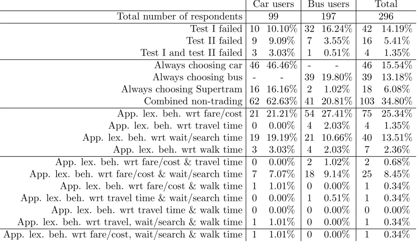
Table 3: Descriptive analysis of South Yorkshire data
Car users Bus users Total Total number of respondents 99 197 296
Test I failed 10 10.10% 32 16.24% 42 14.19% Test II failed 9 9.09% 7 3.55% 16 5.41% Test I and test II failed 3 3.03% 1 0.51% 4 1.35% Always choosing car 46 46.46% - - 46 15.54% Always choosing bus - - 39 19.80% 39 13.18% Always choosing Supertram 16 16.16% 2 1.02% 18 6.08%
Combined non-trading 62 62.63% 41 20.81% 103 34.80% App. lex. beh. wrt fare/cost 21 21.21% 54 27.41% 75 25.34% App. lex. beh. wrt travel time 0 0.00% 4 2.03% 4 1.35% App. lex. beh. wrt wait/search time 19 19.19% 21 10.66% 40 13.51%
App. lex. beh. wrt walk time 3 3.03% 4 2.03% 7 2.36% App. lex. beh. wrt fare/cost & travel time 0 0.00% 2 1.02% 2 0.68% App. lex. beh. wrt fare/cost & wait/search time 7 7.07% 18 9.14% 25 8.45% App. lex. beh. wrt fare/cost & walk time 1 1.01% 0 0.00% 1 0.34% App. lex. beh. wrt travel time & wait/search time 0 0.00% 1 0.51% 1 0.34% App. lex. beh. wrt travel time & walk time 0 0.00% 0 0.00% 0 0.00% App. lex. beh. wrt travel, wait/search & walk time 1 1.01% 0 0.00% 1 0.34% App. lex. beh. wrt fare/cost, wait/search & walk time 1 1.01% 0 0.00% 1 0.34%
Table 3 presents the findings of an initial analysis on the South Yorkshire data. Here, we can observe lower failure rates for Test II than for Test I. This can partly be explained by learning effects, but it should also be noted that due to the proximity of choice set 9 and choice set 12, memory effects potentially also come into play.
Moving on to non-traders, we can see that 46% of car users always choose car, with a further 16% always choosing Supertram. For bus users, the incidence of non-trading is less extreme, and centres on inertia, with almost 20% of bus users always choosing bus as their preferred alternative.
Finally, in terms of apparent lexicographic behaviour, significant shares are only observed for travel cost and for wait/search time, with a quarter respectively an eight of respondents behaving in this manner.
A linear-in-parameters specification of the utility function was again used. Coefficients were specific to the two groups in the data (car users and bus users), while coefficients were also specific to the different modes of travel.
3.2.2 Results
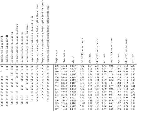
A total of 16 models were estimated on the South Yorkshire data, with results summarised in Table4. The various models differ in terms of whetherproblematic
respondents were included or excluded from the analysis, ranging from a model with all respondents (model 1) to a model where all problematic respondents have been excluded (model 16). In Table 4, we limit our presentation to the results in terms of the main VTTS and model fit indicators. Estimates for other time components often had high associated standard errors, with detailed results available from the first author on request.
Overall, the models produce a much lower VTTS for bus users than for car users, where the latter have a higher standard error, and where the difference between the VTTS for car and Supertram is larger.
The results show that removing respondents who fail either the first or second consistency test leads to gains in model performance, where these gains are more significant in the case of the second test (even though a much smaller number of respondents is affected). Removing respondents failing either or both tests leads to the best results, while in each case, there are slight variations in the VTTS.
Looking next at non-traders, we can see that, compared to the base model, removing car users who are non-traders improves model performance, where, for bus users, this is only the case for respondents always choosing Supertram. Removing car users who always choose car leads to a drop in the car VTTS, while removing car users who always choose Supertram leads to an increase in the VTTS for car as well as Supetram. With Supertram being cheaper than car on average, this should come as no surprise. This can also be used to illustrate the potential upwards bias in the VTTS resulting from political voting by car users who never choose Supertram. For bus users, removing non-traders who always choose bus leads to only small changes, while removing respondents who always choose Supertram leads to a drop in both VTTS measures for bus users, which is a result of Supertram being more expensive than bus. Removing all non-traders from the data leads to a reductions in the VTTS for bus users, and increases in the VTTS for car users, with a doubling for the VTTS for Supertram. This would suggest that despite the higher number of car non traders always choosing car, the impact of car non-traders always choosing Supertram is more significant, and produces a downwards bias in the overall sample.
Table 4: Estimation results on South Yorkshire data (WTP indicators in GBP/hr) Mo del Resp onden ts failing T est I Resp onden ts failing T est II Car users alw ays cho osing car Car users alw ays cho osing Sup ertram Bus users alw ays cho osing bus Bus users alw ays cho osing Sup ertram Resp onden ts alw ays cho osing cheap est option Resp onden ts alw ays cho osing fas test option (tra v el time) Resp onden ts alw ays cho osing fas test option (w ait time/searc h time) Resp onden ts alw ays cho osing faste st option (w alk time) Resp onden ts Observ ations adj. ρ 2 Car VTTS for car users asy . t-rat. ST VTTS for car users asy . t-rat. Bus VTTS for bus users asy . t-rat. ST VTTS for bus users asy . t-rat.
1 X X X X X X X X X X 296 3,552 0.3448 4.82 2.07 2.06 1.83 0.96 3.75 1.10 2.99 2 X X X X X X X X X 254 3,048 0.3546 5.13 2.03 1.86 1.64 1.24 3.97 1.45 3.24 3 X X X X X X X X X 280 3,360 0.3757 4.99 2.54 2.49 1.80 0.94 3.69 0.92 2.59 4 X X X X X X X X 242 2,904 0.3867 5.09 2.36 2.31 1.63 1.19 3.89 1.23 2.89 5 X X X X X X X X X 250 3,000 0.3762 4.17 1.81 2.37 1.81 0.96 3.75 1.10 2.99 6 X X X X X X X X X 280 3,360 0.3728 6.62 1.63 4.07 1.47 0.96 3.75 1.10 2.99 7 X X X X X X X X X 257 3,084 0.3128 4.82 2.07 2.06 1.83 1.01 3.93 1.12 3.00 8 X X X X X X X X X 294 3,528 0.3563 4.82 2.07 2.06 1.83 0.77 4.32 0.84 3.01 9 X X X X X X X X 234 2,808 0.3619 5.62 1.62 3.95 1.39 0.96 3.75 1.10 2.99 10 X X X X X X X X 255 3,060 0.3236 4.82 2.07 2.06 1.83 0.81 4.68 0.85 2.98 11 X X X X X X 193 2,316 0.3376 5.62 1.62 3.95 1.39 0.81 4.68 0.85 2.98 12 X X X X X X X X X 221 2,652 0.2975 9.27 1.41 4.40 1.35 0.83 3.22 0.90 2.31 13 X X X X X X X X X 256 3,072 0.3406 5.70 1.89 2.16 1.69 0.70 4.24 0.76 2.69 14 X X X X X X 199 2,388 0.3161 11.85 1.16 3.66 1.34 0.61 3.57 0.70 2.48
15 X X 169 2,028 0.3192 5.28 1.59 4.19 1.26 0.61 3.57 0.70 2.48
16 117 1,404 0.3982 4.94 2.99 2.50 1.52 0.69 3.74 0.68 2.09
In terms of model performance, overall, the biggest improvements result from removing respondents who fail the second consistency test, where this also largely accounts for the good performance of model 16, the best performing model. This is an indication of the impact that respondents withinconsistent behaviour, no matter how small their number, can have on model results.
3.2.3 Discussion
The analysis on the South Yorkshire data has again highlighted the impact that non-traders and respondents with lexicographic or inconsistent behaviour can have on model results. With the present data, the most important observation relates to the removal of respondents with inconsistent behaviour, while removing non-traders and respondents with apparent lexicographic behaviour also impacts the estimation results. Finally, as with the DATIV data, there are again very little differences in the socio-demographic make-up between the sample for model 1 and the sample for model 16, meaning that the sample after exclusions is no less representative of the data than the original sample.
3.3 First Australian study
Our third analysis makes use of SC data collected in Australia in the context of road pricing initiatives. Respondents were presented with three alternatives, one of which corresponded to a recent trip recorded for the specific respondent. Each respondent was faced with 16 such choice situations, where alternatives were de-scribed by two travel time components, namely free flow travel time (FFT) and slowed down travel time (SDT), and two travel cost components, namely running costs (RC) and tolls (T). Additionally, respondents were presented with informa-tion on travel time variability (VAR). The estimainforma-tion was split into two groups, commuters and non-commuters, with 243 respondents (3,888 observations) in the first group and 223 respondents (3,568 observations) in the second group.
3.3.1 Data analysis and empirical framework
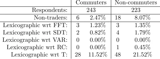
Table 5 presents an initial analysis of the estimation data used in this applica-tion, in terms of non-trading and lexicographic behaviour5
. With the present data, non-trading behaviour was restricted to the reference alternative, with no respondent continuously choosing the second or third alternatives (i.e., the SC alternatives) over all choice situations. The number of non-traders in this data is
5
Table 5: Descriptive analysis of first Australian dataset
Commuters Non-commuters Respondents: 243 223
Non-traders: 6 2.47% 18 8.07% Lexicographic wrt FFT: 3 1.23% 3 1.35% Lexicographic wrt SDT: 2 0.82% 4 1.79% Lexicographic wrt VAR: 0 0.00% 0 0.00% Lexicographic wrt RC: 0 0.00% 1 0.45% Lexicographic wrt T: 28 11.52% 48 21.52%
very low, with rates of 2.47% for commuters and 8.07% for non-commuters. Look-ing next at lexicographic behaviour, non-trivial shares are only observed for road tolls, with 11.52% of commuters always choosing the alternative with the lowest toll, while the rate for non-commuters is almost double that, at 21.52%. Here, it should be noted again that there is a possibility of respondents still trading off other attributes against each other as situations arise where two alternatives both have the lowest toll.
A linear-in-attributes specification was used for the utility functions, with ASCs for the first two alternatives. A second and third group of models were also estimated, including a toll dummy variable for any alternatives with a non-zero toll, where in the third group, this was interacted with respondents’ attitudes towards road tolls. Specifically, respondents were asked to rate how important several aspects of toll roads were to them. A Fishbein multi-attribute model was used in which these ratings were multiplied by the likelihood of the road tolls featuring these aspects. Respondents were divided into three groups, with positive and negative attitude groups as well as a group with indifferent respon-dents. Separate toll dummies were estimated in the former two groups. The aim of including the toll dummy variables is to try and account for strategic voting, hence possibly reducing some of the bias resulting from non-trading and lexico-graphic behaviour. While this creates potential issues with endogeneity, it should be noted that the models estimated here are only used for VTTS calculation and not for forecasting.
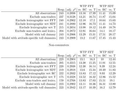
3.3.2 Results
The results of the analysis on the first Australian dataset are summarised in Table
6. The results first of all show that removing non-traders leads to improvements in model performance in both subgroups. As expected, removing the handful of respondents with apparent lexicographic behaviour towards FFT, SDT and RC
Table 6: Estimation results on first Australian dataset (WTP indicators in AUD/hr)
Commuters
WTP FFT WTP SDT Resp. adj. ρ2 vs. RC vs. T vs. RC vs. T
All observations 243 0.2898 13.16 17.39 11.41 15.09 Exclude non-traders 237 0.3128 13.21 16.74 11.87 15.04 Exclude lexicographic wrt FFT 240 0.2902 12.18 17.2 10.64 15.03 Exclude lexicographic wrt SDT 241 0.2880 12.96 16.73 11.41 14.73 Exclude lexicographic wrt T 215 0.2654 13.98 18.12 14.49 18.78 Exclude non-traders and lexico. 204 0.2872 12.91 16.64 14.1 18.17 Model with toll dummy 243 0.2906 13.29 15.31 17.51 20.17 Model with attitude-specific toll dummies 243 0.2909 13.2 11.67 17.45 15.43
Non-commuters
WTP FFT WTP SDT Resp. adj. ρ2 vs. RC vs. T vs. RC vs. T
All observations 223 0.2904 13.1 16.3 10 12.44 Exclude non-traders 205 0.3315 13.38 15.25 11.01 12.55 Exclude lexicographic wrt FFT 220 0.2938 12.38 16.14 9.39 12.24 Exclude lexicographic wrt SDT 219 0.2918 13.6 15.34 10.49 11.83 Exclude lexicographic wrt RC 222 0.2932 13.83 17.12 9.93 12.29 Exclude lexicographic wrt T 175 0.2328 13.52 16.32 12.86 15.52 Exclude non-traders and lexico. 159 0.2768 13.83 17.03 15.51 19.1
Model with toll dummy 223 0.2902 13.11 10.36 16.31 12.89 Model with attitude-specific toll dummies 223 0.2942 13.17 10.39 16.2 12.79
has only very limited effects on fit. On the other hand, removing respondents who always choose the alternative with the lowest toll leads to a clear drop in model performance in both segments, where this also applies in the model that additionally removes non-traders. Including toll road dummies does not lead to significant changes in model performance, whether interacting with attitudes to road tolls or not.
[image:23.612.122.517.188.503.2]in the VTTS measures, though this is relatively small as an effect of the low number of concerned respondents. Removing respondents who always choose the alternative with the lowest road toll has the expected effect of an increase in the VTTS measures where this applies both to the valuations with respect to toll and running costs, suggesting that respondents always choosing the alternative with the lowest toll also bias the running cost sensitivity upwards.
Finally, we look at the results for the models including toll dummy variables. Here, the results are rather mixed. If these terms were to capture strategic voting against tolled alternatives, the expectation would be for a rise in the VTTS measures, especially those calculated against tolls. For commuters, increases in the VTTS measures are observed for SDT, where these are however more significant in relation to RC. For the FFT, there are in fact reductions in the WTP indicators. In the non-commuter models, increases in the VTTS for SDT are again observed with respect to RC, with decreases in the VTTS for FFT with regards to tolls. A possible explanation for these observations could be that untolled alternatives have a higher SDT and that not accounting for strategic voting leads to a downwards bias especially in the sensitivity to SDT.
3.3.3 Discussion
The results from this application are rather more mixed than those from the first two applications, although they still suggest that respondents who behave lexicographically with respect to road tolls can bias the VTTS findings. Here, it should be noted that one of the reasons for the less dramatic effects in this study is the higher number of observations per respondent; presenting an individual with more choice situations (in this case 16) clearly reduces the scope for non-trading and apparent lexicographic behaviour.
3.4 Second Australian study
Our final analysis also makes use of SC data collected in Australia in the context of road pricing initiatives, where the only difference is the inclusion of a third travel time component, namely crawl time (CT). The sample is again split into two groups, commuters and non-commuters, with 304 respondents (4,864 obser-vations) in the first group and 269 respondents (4,304 observations) in the second group.
3.4.1 Data analysis and empirical framework
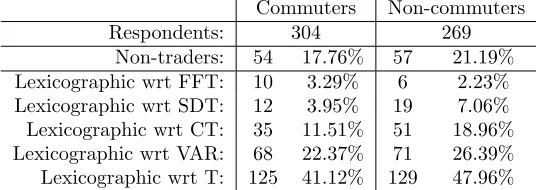
Table7presents an initial analysis of the estimation data used in this application, in terms of non-trading and lexicographic behaviour. Non-trading behaviour was
Table 7: Descriptive analysis of second Australian dataset
Commuters Non-commuters Respondents: 304 269
Non-traders: 54 17.76% 57 21.19% Lexicographic wrt FFT: 10 3.29% 6 2.23% Lexicographic wrt SDT: 12 3.95% 19 7.06% Lexicographic wrt CT: 35 11.51% 51 18.96% Lexicographic wrt VAR: 68 22.37% 71 26.39% Lexicographic wrt T: 125 41.12% 129 47.96%
again restricted to the reference alternative, where the rates were higher than in the first dataset, at 17.76% for commuters and 21.19% for non-commuters. This can partly be explained by less experience with toll roads in the second study area, meaning that respondents are less aware of the potential benefits, increasing the chance for non-trading. Looking next at lexicographic behaviour, significant shares are observed for three attributes, namely crawl time, trip time variability and road tolls. Again, the rates are much higher than in the first Australian study. The modelling methodology used in this study is identical to that used in the first Australian study with the only difference being the inclusion of the new crawl time attribute.
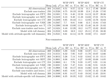
3.4.2 Results
The results of the analysis on the second Australian dataset are summarised in Table 8. The results first of all show that removing non-traders leads to improvements in model performance in both subgroups. On average, removing respondents with lexicographic behaviour from the sample leads to small drops in model performance, with the exception of the case of respondents who always choose the alternative with the lowest trip time variability. Jointly removing non-traders and respondents with apparent lexicographic behaviour leads to a small drop in model performance. Including toll road dummies does with this dataset lead gains in model performance, where the extra cost of accounting for respondents’ attitudes is apparently not justified.
Table 8: Estimation results on second Australian dataset (WTP indicators in AUD/hr)
Commuters
WTP FFT WTP SDT WTP CT Resp. adj. ρ2 vs. RC vs. T vs. RC vs. T vs. RC vs. T
All observations 304 0.2445 8.51 9.57 12.54 14.1 17.86 20.08 Exclude non-traders 250 0.2526 8.75 10.19 10.99 12.8 15.38 17.92 Exclude lexicographic wrt FFT 294 0.2481 7.55 8.48 12.58 14.13 18.57 20.86 Exclude lexicographic wrt SDT 292 0.2419 8.18 9.49 11.23 13.03 17.01 19.74 Exclude lexicographic wrt CT 269 0.2389 8.95 10.43 11.1 12.93 13.76 16.03 Exclude lexicographic wrt VAR 236 0.2567 7.7 9.81 9.66 12.3 13.84 17.63 Exclude lexicographic wrt T 179 0.2390 10.08 13.09 11.92 15.48 16.19 21.02 Exclude non-traders and lexico. 167 0.2424 8.48 12.29 10.2 14.77 13.82 20.02 Model with toll dummy 304 0.2552 8.88 16.9 13.2 25.11 17.55 33.38 Model with attitude-specific toll dummies 304 0.2521 8.61 12.14 12.78 18.02 17.5 24.67
Non-commuters
WTP FFT WTP SDT WTP CT Resp. adj. ρ2 vs. RC vs. T vs. RC vs. T vs. RC vs. T
All observations 269 0.3022 5.88 8.03 9.06 12.37 11.1 15.16 Exclude non-traders 212 0.3151 6.32 7.95 9.37 11.78 10.07 12.66 Exclude lexicographic wrt FFT 263 0.3013 5.26 7.14 9.32 12.64 11.13 15.11 Exclude lexicographic wrt SDT 250 0.3001 6.08 8.01 8.27 10.89 10.68 14.05 Exclude lexicographic wrt CT 218 0.3063 6.1 7.76 9.33 11.87 8.91 11.34 Exclude lexicographic wrt VAR 198 0.3231 5.82 7.47 9.24 11.86 9.55 12.25 Exclude lexicographic wrt T 140 0.2908 7.36 10.17 10.61 14.66 12.01 16.59 Exclude non-traders and lexico. 127 0.2965 6.65 8.94 10.1 13.59 11.42 15.36 Model with toll dummy 269 0.3109 6.91 14.17 9.43 19.34 11.65 23.91 Model with attitude-specific toll dummies 269 0.3080 6.35 10.35 9.22 15.02 11.43 18.62
The removal of respondents with apparent lexicographic behaviour in rela-tion to the various travel time components has very much the expected effects, with a reduction in the associated VTTS measures. In other words, including respondents who always choose the fastest alternative leads to an upwards bias in the VTTS measures. Including respondents who always choose the alternative with the lowest travel time variability also on average leads to an upwards bias in the VTTS measures, which is consistent with intuition. Removing respon-dents who always choose the alternative with the lowest tolls leads to an upwards
correction of the VTTS measures calculated relative to tolls, which highlights an overestimation of the toll sensitivity when including such respondents in the model. Jointly excluding respondents with non-trading or apparent lexicographic behaviour leads to bi-directional changes across the various VTTS measures.
Finally, we look at the results for the models including toll dummy variables. Here, the results are far more promising than with the first Australian dataset. Indeed, we can see that there is a clear increase in the VTTS measures calculated with respect to toll sensitivity. This shows that the inclusion of the toll dummies leads to a downwards correction in the estimated toll sensitivity, which can be seen as a reduction in the effects of strategic voting.
3.4.3 Discussion
The findings from the second Australian study are slightly more interesting than the results from the first study, showing strong effects of non-trading, apparent lexicographic behaviour and strategic voting. The most interesting finding relates to the correction effects resulting from the use of penalty terms associated with tolled alternatives.
4
Summary and conclusions
In this paper we have discussed a number of issues relating to the pre-analysis and cleaning of stated choice data. We have argued that this process is in fact considerably more complex and challenging than many in the field have hith-erto acknowledged. The key issue is the ability of a pre-analysis to identify and characterise in SC data response patterns that are or are not consistent with the assumptions of a given model being used to analyse the data. At present our capability to systematically discriminate between different regimes of response is rather rudimentary and pre-analysis is typically limited to the application of a number of ad-hoc procedures for the identification of non-trading, lexicographic and inconsistent response patterns. The impact of these ad hoc procedures on model estimation results is far from clear.
The overall conclusion from this work is that there is an urgent need to develop more theoretically coherent methods of response regime classification. Recent developments in the literature on information processing strategies provide some useful insight into how this work might be taken forward. Finally, where possible, the inclusion of explicit tests for consistent behaviour in SC surveys can be a great asset in the pre-analysis and cleaning of SC data.
References
Bierlaire, M. (2003) BIOGEME: a free package for the estimation of discrete choice models, Proceedings of the 3rd Swiss Transport Research Conference,
Monte Verit`a, Ascona.
Blume, L., A. Brandenburger and E. Dekel (2006) An overview of lexicographic choice under uncertainty,Annals of Operations Research,19(1) 229–246.
Burge, P. and C. Rohr (2004) DATIV: SP Design: Proposed approach for pilot survey, Tetra-Plan in cooperation with RAND Europe and Gallup A/S.
Campbell, D., W. G. Hutchinson and R. Scarpa (2006)Lexicographic Preferences in Discrete Choice Experiments: Consequences on Individual-Specific Willing-ness to Pay Estimates, Working Papers 2006.128, Fondazione Eni Enrico Mat-tei.
de Borger, B. and M. Fosgerau (2007)The Trade-Off Between Money and Travel Time: A Test of the Theory of Reference-Dependent Preferences, Journal of Urban Economics, forthcoming.
Deshazo, J. R. and G. Fermo (2002) Designing choice sets for stated preference methods: the effects of complexity on choice consistency, Journal of Environ-mental Economics and Management,44(1) 123–143.
Fosgerau, M. (2006) Investigating the distribution of the value of travel time savings,Transportation Research Part B: Methodological,40 (8) 688–707.
Foster, V. and S. Mourato (2002) Testing for consistency in contingent ranking experiments,Journal of Environmental Economics and Management,44, 309– 328.
Fujii, S. and T. Garling (2003) Application of attitude theory for improved pre-dictive accuracy of stated preference methods in travel demand analysis, Trans-portation Research Part A: Policy and Practice,37(4) 389–402.
Garling, T., R. Gillholm and A. Garling (1998) Reintroducing attitude theory in travel behavior research: The validity of an interactive interview procedure to predict car use, Transportation,25, 129–146.
Hensher, D. A. (2007)Joint estimation of process and outcome in choice experi-ments and implications for willingness to pay, Journal of Transport Economics and Policy, forthcoming.
Hess, S., J. M. Rose and D. A. Hensher (2008) Asymmetrical preference forma-tion in willingness to pay estimates in discrete choice models, Transportation Research Part E: Logistics and Transportation Review,44(5) 847–863.
Kuriyama, K. (2005) Strategic effects on stated preferences for public goods: A theoretical and experimental analysis of the contingent valuation survey, The Waseda Journal of Political Science and Economics,359, 83–92.
Mehta, R., W. L. Moore and T. M. Pavia (1992) An examination of the use of unacceptable levels in conjoint analysis,Journal of Consumer Research,19(3) 470–476.
Polak, J. W. (1994)Supertram Monitoring Study: Report of Before Surveys, TSU Ref 812, Transport Studies Unit, University of Oxford.
Puckett, S. M. and D. A. Hensher (2007)The role of attribute processing strate-gies in estimating the preferences of road freight stakeholders, Transportation Research E, forthcoming.
Rekola, M. (2003) Lexicographic preferences in contingent valuation: a theoretical framework with illustrations, Land Economics,79(2) 277–291.
Rosenberger, R. S., G. L. Peterson, A. Clarke and T. C. Brown (2003) Measuring dispositions for lexicographic preferences of environmental goods: integrating economics, psychology and ethics,Ecological Economics,44, 63–76.
Sælensminde, K. (2001) Inconsistent choices in stated choice data. use of the logit scaling approach to handle resulting variance increases,Transportation,28(3) 269–296.
Sælensminde, K. (2002) The impact of choice inconsistencies in stated choice studies,Environmental and Resource Economics,23, 403–420.
Train, K. and W. W. Wilson (2007)Estimation on stated-preference experiments constructed from revealed-preference choices, Transportation Research Part B: Methodological, forthcoming.
Verplanken, B. and H. Aarts (1999) Habit, attitude and planned behaviour: Is habit an empty construct or an interesting case of goal-directed automatic?,
European Review of Social Psychology,10, 101–134.