Fitting distributions to diameter and height data from even-aged stands of Pinus radiata

FROM EVEN-AGED STANDS OF PINUS RADIATA

by

Robert Ian Forrester

A thesis submitted to the Australian National University

/

as part requirement for the degree of Master of Science.

C O N T E N T S

1 2

3 4 5 6

7

8

9

C O N T E N T S ... (i) ACKNOWLEDGEMENTS . ... (ii)

SUMMARY ... (iii) Introduction ...

The Data ... The 8i - $2 Plane ... Maximum Likelihood Estimation ... Kolmogorov-Smirnov Test for Goodness of Fit . Results of Maximum Likelihood Estimation and the Test for Goodness of Fit ...

(a) The Diameter Data ... (b) The Height Data ... Estimation of Bivariate Distributions . . . . Results for SUT5 D i s t r i b u t i o n ...

D jD

D i s c u s s i o n ... .. . . . REFERENCES . . .

TABLES and FIGURES

1

4

8

12 23

UlJ

Acknowledgements

I thank Dr I. Ferguson who suggested the topic,

provided the data and gave many valuable suggestions. I also thank Mr P. Winer for several useful

Summary

The data used in this study were obtained from forty even-aged yield plots of P. radiata from the Kowen plantation in the Northeast corner of the Australian Capital Territory. The trees were planted between 1927 and 1944 and measurements of diameter and height were made on all plots on three or more occasions between 1955 and 1971 inclusive.

In this dissertation the six univariate distributions, normal, lognormal, gamma, beta, Weibull and Johnson's SD ,

D

are fitted to the 149 measurement data by plot data sets. As a means of comparing the relative fits of these

distributions, sums of the ranks of the maximized log-likelihood values, for the six distributions on 149 data sets, were

obtained. The Kolmogorov-Smirnov goodness of fit statistic was also calculated for these distributions and the sums of

the ranks of these obtained. There was very little agreement between these two methods of assessing the relative adequacy of the distributions of interest, for either the diameter or the height data. Hence it appeared that, for this data, there was little difference overall between any of the six distributions.

U VJ

Bivariate Sß (Sgg distribution) distributions and

to diameter data in both even-age and mixed-age stands of

trees. See for example Bailey and Dell (1973), Bailey

(1974) , and Schreuder and Swank (1974) . There are several

references to earlier work in these papers. Bailey and

Dell, and Bailey discuss in detail the fitting of two and three parameter Weibull distributions to diameter data. Bailey states that diameter is generally well correlated

with other variables of interest such as tree volume. He

asserts that the quantification of the distribution of diameter, and its relationship to site, stand composition, age and density is often valuable for both economic and biological purposes.

Schreuder and Swank used the two parameter Weibull distribution to summarize diameter, basal area, surface area, biomass and crown profile data for several different

ages of white and loblolly pine plantations. They found

that the data for these variables were easily summarised by this one distribution in a theoretically consistent fashion. This was evidently not possible with the normal and gamma distributions, and the lognormal gave less satisfactory

results. They then assert that the distribution function

should prove useful in modelling tree stands since only the parameter values need to be changed over time for the above

variables. The change in these parameter values, they say,

More recently, Hafley and Schreuder (1977), have fitted six distributions to both diameter and height data for even- aged stands of shortleaf pine, longleaf pine and loblolly

pine. The distributions they chose were the normal, lognormal, gamma, beta, Weibull and Johnson's Sg. They conclude that

overall the Johnson's Sg distribution gave the best performance in terms of the log likelihood criterion.

In another paper Schreuder and Hafley (1977), extend their results from the univariate work to an examination in detail of the bivariate Johnson Sgg distribution in its application to diameter/height data. The rationale for endeavouring to fit bivariate distributions to diameter/ height data from forest stands is explained quite succinctly in the Introduction to Schreuder and Swank's paper:

"An important problem in forestry is the prediction of stand yields in volume on the basis of stand age, productive capacity of the site, and stand density.

Forest managers are interested in studying the effect of such stand management practices as thinning and fertilization on volume in pulpwood, sawtimber, and

veneer. The volume in each of these products is heavily dependent on tree diameter and height distributions.

For example, a given stand volume consisting of small trees may be entirely pulpwood; whereas, the same

volume in a few large trees may be primarily sawtimber. Hence, there is considerable interest in the successful fitting of a bivariate statistical distribution to

height - d iameter relationship to estimate average height per diameter class and thence volume. Although this

latter approach is satisfactory in many ways, it ignores the fact that height can vary considerably for a given diameter. This is especially important in older,

commercially more important stands. Hence, the possibility of generating a bivariate distribution of diameters and heights for a stand would often be of interest to

The Data 2.

The data were obtained from forty* even-aged yield plots of P. vadiata from the Kowen plantation in the Northeast corner of the Australian Capital Territory

(A.C.T.). The trees were planted between 1927 and 1944 and measurements of diameter and height were made on all

plots in 1955/56, 1962 and 1971, with additional measurements made on some plots in 1958 and 1967. In Table 1 the plot

code, the year of planting, the measurement dates and the number of trees are given.

Measurements (in cm) of diameter at breast height over bark (DBHOB) were made using a girth tape; breast height

is 1.3m (4.25 feet) above ground level. Total height (in m) of the trees was measured by Haga Altimeter, with two readings being taken from different positions. In the case of leaning trees, the vertical component was taken as the tree height. The measurements of tree diameter are

quite accurate. The height readings, however, have quite large measurement errors associated with them. There were 8056

pairs of measurements made on tree height and of these 253 (3.14%), the difference between the two values was greater than 1.5m. In 27 measurements (0.34%) this difference

between the two heights was greater than 3m. As expected most of the more disparate readings occurred with plots containing older and taller trees. One obviously erroneous measurement of tree height was corrected in the data set.

* The last few sets of data were lost from plot

carried out on a plot until the trees were 15 years of age. The thinning that was carried out in 1956 was quite light. This can be seen by looking at the tree numbers per plot given in Table 1. Usually the trees

that were thinned, on each occasion, were those with the smallest diameter. In some instances thinning could remove up to 50% of the trees from a plot. The time when the plots were thinned relative to the time of measurement of the plots may have a profound effect on the nature of the distribution of the diameter and height values. If several years had elapsed between the time of the last thinning and the

measurement of the diameter and height then the distributions of these variables might be expected to have stabilised again for that plot. Generally speaking the plots were thinned after the measurements were made so that thinning should not have a profound affect on the diameter and height distributions.

There is one occurrence in the data set where a plot was measured on two consecutive days, before and after thinning. The plot involved is 350601, which was measured on 13/5/71 when it had 68 trees and also on 14/5/71 when

it had 19 trees. Histrograms for the distribution of

diameter and height before and after thinning are given in Figures 1 to 4. The change is more noticeable for the

6

distribution after thinning. It is also apparent that it is not only the smallest diameter trees that have been thinned on this plot. However, in general it is predominantly the smallest diameter trees that are removed when thinning a plot.

In a number of sets of data there appeared to be an abnormally large number of height measurements where both readings were the same. This siutation is illustrated in Figure 5, which is a histogram of the proportion of trees on a plot for which both the height readings are the same. The plots and measurements dates involved are listed in

iable 2. There are two possible explanations for this;

either there was only one height measurement taken in the field, or there were two readings taken, but only the mean value

recorded. In both instances the recorded height was coded twice on the data sheets prior to the entry of the data into the computer. Hence the height data for these data sets will have greater variability than that for the other data sets.

All subsequent data analyses have used the mean of the two tree height measurements as the observed value of

tree height.

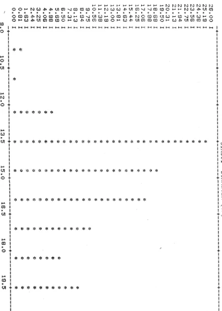
In order to obtain some insight into the distribution oi the data, histograms were plotted for a few of the data sets. Figures 6 and 7 are histograms for the diameter and height values for the first plot, 31A501 planted in 1941 and measured 23/1/56. Histograms for another plot, 31A601 planted in 1941 and measured 22/1/58 are given for diameter and height variables in Figures 8 and 9 respectively. None of the Figures appear to represent a normally distributed set of data, although, save for some slight bimodality, the

figures we can also see that we have to deal with data that can be either positively or negatively skewed.

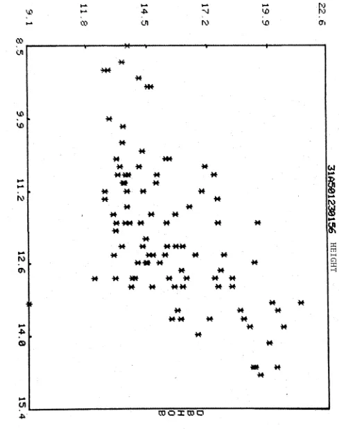
To illustrate the relationship between the diameter and height measurements, a bivariate plot for the first set of data (31A501, measured 23/1/56) is given in Figure 10.

VJ

3. The ß]-ß2 Plane

Before proceeding to fit univariate distributions to the diameter (DBHOB) and height data, we should look

in some detail at the sample moments for this data and endeavour to assess the suitability or otherwise of these distributions. The distributions that we will look at are

the normal, lognormal, gamma, beta, Weibull and Johnston's SB *

t h

Let us define as the r sample moment about the mean of the distribution of a random variable x with density function f(x). That is

f 00

yr = I (x-E (x)) 1 f (x) dx .

- OO

In addition to the mean yi1 and the variance y 2, we have two coefficients which are functions of lower order moments. The first is the skewness coefficient

/FT

which

3/ 2

is defined as y 3/C y 2) , and the second is the kurtosis 2

coefficient £2 defined as yu/yi2 . Skewness measures the departure of the distribution from symmetry about the mean, with negative values of

/FT

indicating a distribution with a long tail to the left, and positive values indicating a distribution with a long tail to the right. On the other hand kurtosis is considered to be a measure of the peakedness of a distribution with larger values of £2 indicating a

more peaked distribution.

The moment estimators of

/FT

and $2, for a sample of size n , are

/F z i (xi - X) 3

{Xi(Xi - X) 2 }3/2

for /bi and b 2 respectively, Fisher (1970).

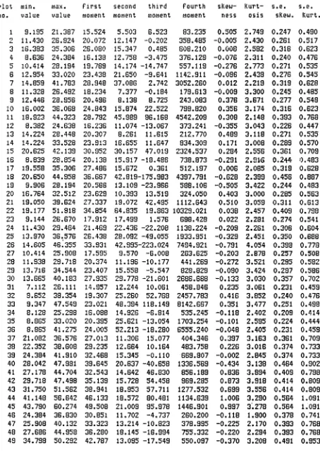
Values of the sample moments and the values of /bi and b 2 with their standard errors, for the diameter and

height data from Kowen are given in Tables 3 and 4 respectively. In these Tables the plot codes used in Table 1 do not appear. However the plots are in the same order, with the results for

all measurement dates on a plot given consecutively. That

is the first three lines in Tables 3 and 4 are the results for the three measurement dates on plot 31A501, and so forth. There are a couple of points to notice in these Tables.

Firstly for the height data, almost all (84%) the values of

Sbi are negative, whereas for the diameter data, both negative

and positive values occur almost equally often (44% to 56%). Secondly, it is fairly obvious that for the majority of the 149 data sets for both variables the value of the skewness coefficient would not be significantly different from zero. In order to demonstrate the range of the skewness-and kurtosis coefficients covered by the various statistical distributions, authors have often used a graph of the Bi-ß2

plane; for example Johnson and Kotz (1970a) and Hafley and

Schreuder (1977). The sample values of bi and b 2 for the

diameter data have been plotted in Figure 11. In this

diagram I have indicated the possible values of and ß2

There is an impossible region on this graph where it is

mathematically impossible for certain combinations of ßj and ß2 to occur. The normal distribution is represented by a point in this plane, whereas the lognormal, Weibull, and gamma distributions are all represented by lines, thus illustrating their greater flexibility over the normal in their ability to adequately represent data. The beta

distribution is even more flexible since it is represented in the ßj - ß2 plane by the area between the impossible region line and the gamma distribution line. The Sg distribution is one of three distributions proposed by Johnson (1949a).

These distributions are transformations of a standard normal variate, and together the three of them span the ßj - ß2 plane. The Sg distribution spans the area between the

impossible region line and the lognormal line; the Sg

distribution is the three parameter lognormal distribution; and the Sy distribution covers the remainder of the 31 - g2 plane. Therefore the Sg distribution is a little more

flexible than the beta in the range of values of skewness and kurtosis that it can represent.

It is worth noting at this stage that the gamma and lognormal distributions can only adequately represent

positively skewed data. From Figure 11 we are not able to discern which points represent negatively skewed data and which represent positively skewed data.

[image:16.552.55.512.36.785.2]

is these points are from sets of data where the skewness is relatively small compared to the kurtosis. This situation

does not appear to occur with the data of Hafley and Schreuder. Table 5 enumerates the plots and measurement dates where

[image:17.552.75.524.112.776.2]

4. Maximum Likelihood Estimation

To enable comparisons to be made between the fit of each of the distributions of interest to the data, we will fit each of them using maximum likelihood. We can compare values of the maximized likelihood function for these

distributions and assess their relative fits. Since the calculation of the likelihood function itself is quite

difficult, we will concentrate as is usual on the log of the likelihood, which has a maximum at the same parameter values as the likelihood.

(a) Normal distribution

The probability density function (p.d.f.) for a normal distribution with mean y and variance a*2 is

The likelihood function for a random sample of size n is

f(x) = -t — -jj{(x-u)/a} / o __ _ ^

2

- 0 0 < X , y < ° o , a 2 > 0 .

L = n i = 1

n

Hence the log of the likelihood is

£ in 2tt- n £no

D ifferentiating £ with respect to the parameters y

and 0 2 , and equating the resultant two equations to zero, we

can solve to obtain the well known maximum likelihood

estimates for the normal distribution,

Ä n

y = E X .

1 = 1_____

n

-1 n

a 2 = — E ( X . - y )

i = l

(b ) Lognormal distribution

For a three parameter lognormal distribution with

location parameter 0 we have the p.d.f.

1 ' 7a2Wn(x-0)-y>2 f(X) = --- HI— e

( x - 0 ) / 2 r r a

x > 0 , - °°< y <°°, a 2>0 .

If 0 were known (usually it is zero), we then have a

two parameter lognormal distribution. That is, if z^=£n(x^-0)

then we obtain the density function

f(z) 2 G 2

(z-y) e Z / 2 TT a

Hence the likelihood for a random sample of size n is

n

n

i = l

1

M-and we obtain the M . L . E . ’s of the parameters of

y _n1_

n E i= 1

Z .

i

n E i = 1

( Z j - v) 2

If 6 were unknown we have the likelihood

n , - Y J 2 Un(X.-e)-y) 2

L = n ---— — e

i = l ( X ^ - 0 ) / 2tt ct

From the log of this likelihood we can obtain the equations

for estimating the parameters y and a 2 of

1 n

y = y(0) = — Z [£ n ( X ^ - 0)]

i = 1

a 2 = a 2 (0) = “■ E { £ n ( X i - 0 ) -y (0) }2

i = 1

Johnson and Kotz (1970a) suggest that these could be

solved by taking a sequence of values of 0, calculate the

m a x i m i z e d l o g -likelihood corresponding to each, then try

to estimate n umerically the value 0 of 0 which maximizes

the maximized l o g - l i k e l i h o o d . They refer to a paper by

Hill (1963) who has shown that this procedure runs

into trouble since the max i m i z e d l o g - 1 ikelihood tends to

infinity as 0 tends to min ( X j ,X 2 ,..•,X ). The M.L.E. of

should solve the above two equations subject to the constraint that

n X . - 0 •, n , .

z s,n[n T gy]

( x i -e)

= -

z

( x . - e )

1

O 2 (0)

i = 1 1 J i = 1

where G(0) = £ n [ n (X^-0)]n .

i = l

This reduces to

__1_

o 2 (0)

E (X-- 0)~1 [ £ n ( X •-0)-y(e)] + E (X.-0)

i=l 1 1 i=l 1

0

where y(0)

~

z

sin(x.-e)

n i = l 1

(c) Gamma distribution

The three parameter gamma distribution, with location parameter 0 has p.d.f.

- (x-0)/ß

f(x) = (x-0)“ "1

-5----ß r ( a )

a , ß > 0 x > 0 ,

and where r ( a ) is the gamma function.

When 0 is 0 (the most usual case) we obtain

xa-!e-x/ß f(x)

and this has likelihood

i=l ßa T(a)

The log likelihood is then

1 n n

£ = E X. -n Jin r (n) + (a-1) E £nX. - an£nß

3 i = l 1 i=l 1

and we can obtain the two equations (in the two unknown

parameters)

-1- E £nX- = £nß + p(a)

n • i i

i = l

a $ X.

l

where q ('. ) is the digamma function, viz. q (a)

r

(a)

r

(a)

Eliminating ß we obtain

T 1 i /N

— E £ n X . - £n X = q(a) -£n a ,

i = l

and since

1

1 n _ n

£n X - - E £ n X . = £nX - £nn(X.)n

n . i . ) i J

l - l i = l

we have

arithmetic mean (X., , . . . ,X )

--- --- h—1 = p n n

approximation is due to Thom (1968) and is as follows:

- 1 n

if Y = £nX - - E £ n X .

n . , i

i = l

then an approximation for a is

a = iy (1 + /1+ jY) .

If 8 is unknown then we would have to obtain the

M.L.E.'s of the three unknown parameters from the following equations obtained from the log-1 ikelihood.

n

E £n (X - - 0) - n £ n ß - n q (a ) = 0

i = l . 1

n

E (X. - 0) ~ n a 8 = 0 i = l 1

E (X--0)"1 + n / { 8 (a-1)} = 0

i = 1 1

1

«

(d) Beta distribution

When the range parameters a and b are unknown, we have

the p.d.f. for a beta random variable of

f(x) 1____

B(p,q)

(x-a)p ~ 1 (b-x)p " 1 ,

(b-a)p+p_1

a < x < b

p, q > 0,

where B(p,q) is the beta function.

For a random sample of size n the likelihood function is

L = n n i = l

1___ (Xi -a)p_1 (b-Xi)q ‘ 1

(b- a)p+c*~ 1

and hence the log-likelihood is

£ = -n £n[B(p , q) ] + (p-1)

n

+ (q-1) E £n(b-X.) -

i = l 1

n

z n (X - - a)

i = 1

n ( p + q - 1 ) £n(b-a)

If the values of the range parameters a, and b are known

then we obtain the likelihood equations for the parameters

p and q :

a a -a -j n X . a

b(p) - M p + q) = S ^

i = l

* Ä ~ l n b-X.

4- (q) - i|i(p+q) = „ ~)

i = 1

Johnson and Kotz (1970b) state that we can solve these

equations iteratively for p and q. They further state,

that if a and b are unknown, then the M.L.E.'s of all

four parameters can be obtained by using a succession of

trial values of a and b, until a pair (a,b) for which the

max i m i z e d l o g - 1 ikelihood is as great as possible, is attained.

(e ) Weibull distribution

The p.d.f. for a three parameter Weibull d i stribution

is

f(x ) = c ( x - e )L ~ ]- e - [ (x- 6) /b ] c

b c

where 0 is the location parameter, x > 6 > 0 ,

b is the scale parameter, b > 0 ,

and c is the shape parameter, c > 0 .

The likelihood for a random sample from the two parameter

Weibull d i stribution with 6=0 is

n

n

i = l

cX.

l

c - 1 [Xi/b]

Bailey and Dell (1973) say that the M . L . E . 's of the parameters

can be obtained by iteratively solving

n n Ä .

[ E X . L i>n X. ] / [ E X . C ] - i

i=l i=l 1 c

n

E Än X i = 1

for c and then solving

n c

[-1- E X . ]C

n i = 1 1

zu

Details of the estimating equations for the three parameter

case are given in Harter and Moore (1965). They outline

an iterative technique for solving these equations.

The l o g - 1 ikelihood for the three parameter model is

n n X . - 0

i = n Hn c - nc ln b + E (k-1) £n (X . - 0) - E (— -r--) C

i=l 1 i=l D

(f) Johnson's Sg distribution

Johnson (1949 a) proposed three distributions, which

together span the 3 1~ 32 plane. As m e n t ioned earlier

the one we are interested in is the Sg distribution.

Let z = y + 6 £n )

where z is a unit normal variable and £ < x < % + X .

Using the change of variable technique we can obtain the

p.d.f. for the variable x.

That is f(x) 1__ 6 A_________

/ 2 7r (x-£)(£+X-x)

i[Y

+

6^n(I^ ) i 2

where the variable x is said to have and Sg distribution.

When the range parameters £ and X are both known, then

Johnson has shown that closed form estimates of y and 6

can be obtained.

v i z . y 6 1

s where y

1 n

n E

i= 1 *

(Yi-y) 2

£n

x .

1- K

? + X - x i

The likelihood function for a random sample of

size n from an Sg distribution is

L

n

n

i = l

_____ 5X___________

/27(Xr S) (C + X-Xp

e

I [ Y + ä £n (

^+A-X.•)]

2

The l o g -likelihood is

n

£ = n £n Ü - y £n 2ir - 2 Än(X.-£)

i = i

n

E £ n U + A-X.)

i = l 1

1

2

n X.-C 2

•

V Y +

5 in^FlCX7)]

1 = 1 ^ 1

(g) General method of estimation

For each of the distributions above, where closed form

m a x imum likelihood estimates of the parameters do not exist,

a specific iterative me t h o d can be used to obtain these

estimates. However, rather than write a program for each

of the iterative methods outlined above, it was decided to

reduce the amount of programming required and utilize a

general m i n i m i z a t i o n routine. The minimiz a t i o n technique

used is the simplex method of Neider and Mead (1965). This

has been progra m m e d by Shaw (1971, unpublished) in a

Fortran subroutine called MINIM. The maximum likelihood

estimates are the parameter estimates which minimize

"minus the log likelihood function". Simplex is not the

fastest m i n i m i z a t i o n technique available (and it would

techniques mentioned earlier, but it does have the advantage that partial derivatives of the function being minimized, with respect to the parameters, do not have to be provided.

If requested, MINIM will fit a quadratic surface in

the region of the minimum. The coefficients of this polynomial form the Hessian matrix of the second derivatives of the

function being minimized. It is well known that if the

distributions to the diameter and height data, we also

used a Kolmogor o v - S m i r n o v test, Massey (1951) in addition

to the value of the m a x imized likelihood.

Suppose we have a popul a t i o n which is thought to

have some specific cumulative frequency distribution function

Fq(x). That is, the value of Fq(x) is the propor t i o n of

individuals in the population having values less than or

equal to a particular value x. For a random sample of N

observations we would expect its cumulative step function

to be quite close to the specified distribution function

Now Fq(x) is the p o pulation cumulative distribution

function, and if S^(x) is the observed cumulative step

of observations less than or equal to x ) , then the

sampling d i stribution of d = maximum | F^ (x) - S^T (x) | is

known, and is independent of Fq(x), if Fq(x) is continuous.

Mas s e y tabulated critical points for the distribution

of d for various sample sizes.

The population cumulative distribution functions for

the six distributions of interest were computed using

the following methods.

(i) N o r m a l We have $ (u) = P (U < u)

function of a sample (S^(x) = — , where n is the number

1__

/ 2u u

where U has a standard normal distribution. For a normal distribution X with mean y and variance a2 , we have P^(X < x) = P (U < —^ ) . An approximation due to Hastings is

1 2 3 ZL - 4

<3? (u) # 1 - ~ 2 (1+ a 1 u + a 2 u + + )

where a1=.196854, a2=.115194, a3=.000344, a4=.019527 and u > 0.

(ii) Lognormal We can obtain the cumulative distribution from that for the normal, using the transformation

U = (logx - y)/a.

(iii) Gamma Johnson and Kotz (1970a) give the following approximation, due to Wilson and Hilferty (1931), for the X2 distribution;

Pr (x^ < x) = $[{(x/y)3 - 1 - }/9y/2 ]

We can obtain the result for the general gamma distribution, x — 0

using the transformation y = . That is x = 0 + 3y . Note that y=2a and that 0=0 for the two parameter gamma distribution. The approximation is very good if y>30

(iv) Beta Johnson and Kotz (1970b) suggested an approximation to the incomplete beta function ratio.

However this approximation breaks down completely if either or both of p and q are less than 0.5. This does occur

in a few data sets and so it was necessary to use a more exact procedure, I used the IMSL routine MDBETA which is a Fortran program based on the Collected Algorithms from A.C.M., algorithm 179, Ludwig (1963).

(v) Weibul1 The cumulative distribution function is F (x) =1-exp[ - { (x-9)/ct }c] , Johnson and Kotz (1970a).

(vi) Johnson's Sg We can obtain the cumulative distribution function from the normal using the transformation

U =y +6 log (—~— — ), where £ = 0 for the diameter data and + A - X

2 6

6. Results of Maximum Likelihood Estimation and the Test for Goodness of Fit

The minimum value for DBHOB was set at 0 cm for all data sets. Further the minimum value for height was set at 1.3 m; that is the height at which the diameter measurement was made. These seem reasonable lower bounds

as we are trying to fit distributions to a number of data sets on different aged trees. Hence we are estimating two parameters for normal, lognormal, gamma and Weibull, and three parameters for the beta and Johnson’s

distributions. Therefore estimates of the parameters of the normal and the lognormal and the values of their

log -1ikelihoods could be obtained directly, and for the gamma the Thom approximation could be used. For the other three distributions the parameter estimates and the values of the maximized log-1ikelihood were obtained using MINIM.

Most of the computations carried out in this section were performed on a PDP 11/34 computer.

(a) The Diameter Data

Initially the second range parameter (upper limit for the range of the data values), for the beta and

distributions was set to be maximum (observed diameter on the plot) + 5 cm. The values of the maximized log-likelihood for all six distributions and all 149 sets of data were

data set the six 1o g -1ikelihood values were ranked (largest to smallest) and the sum of these ranks calculated for

each distribution. The values obtained were: normal, 434;

lognormal, 587; gamma, 472; beta, 429; Weibull, 644;

Sp,, 563. Hence we conclude that overall the beta distribution

was the best performer, the normal the next best and so on.

The Kolmogorov-Smirnov (K-S) statistic d was calculated

for all distributions and all plots. Values of d were ranked

(smallest to largest) and the sums of these ranks obtained

for each distribution. The values were: normal, 406;

lognomal, 457; gamma, 413; beta, 556; Weibull, 624;

Sg, 673. From these summed ranks we could conclude that

the best performer was the normal distribution, the gamma the next best, and so on.

If we now estimate the second range parameter, for the beta-and Sß distributions, we encounter difficulties

with several data sets. Not suprisingly the problems occur

where there is positive skewness in the data. The log-

likelihood surface has a long ridge where it is close to its maximum value for a wide range of values of the range

parameter. In order to overcome this problem the values

of the range parameter were constrained to lie between the maximum observed diameter + 0.0001 cm, and an upper limit

derived from the relationship

Since there was no relationship that we could find in the literature, relating maximum tree diameter on a plot to tree age for p. radiata, it was necessary to obtain a suitable relationship from the data we had available.

This was done as follows. In Figure 13, the maximum observed tree diameter for each of the 149 data sets was plotted

against tree age. Since we were interested in setting an upper bound for diameter on plots of a certain age, then

eight points, arrowed in this figure, were chosen and a Mischerlich curve was fitted. This seemed to be a

reasonable model for this data with no apparent systematic trend in the residuals from the fitted model. In order to be satisfied that we were setting a reasonable upper bound for the iteration procedure to work within, an addition of 10 cm was made to the value of the maximum diameter obtained from the Mischerlich model. This upper bound is plotted on Figure 13.

For the beta distribution, the estimated value of the second range parameter, b, was almost identical to the

value obtained for maximum diameter from the above relation­ ship (6.1) in 74 of the 149 data sets. In all but two of these 74 data sets, the data had positive skewness. For the two with negative skewness, (data sets 87 and 88), the estimated value of skewness was just less than zero.

were data sets where the estimated second range parameter from the iterative procedure, was the maximum diameter for trees of that particular age on that plot, (obtained from the equation 6.1 given above). Recall that the plots consist of equal aged trees. It would seem that for

these 23 data sets, there is a long ridge in the likelihood surface, where a large change in the magnitude of the

second range parameter will have very little effect on the value of the log-1ikelihood. This is quite a common problem encountered when fitting nonlinear models to data. Also it is quite likely, that for some of the other data sets where the second range parameter estimate was the same as the maximum plot diameter, that there is a ridge in

the log-likelihood surface. However the iterative

procedure in MINIM did converge in our situation where we were constraining the value of the second range parameter. Fortunately for the diameter data and the beta distribution there are not to many instances where MINIM failed to

converge satisfactorily.

Another serious problem is one that arises when the quadratic surface near the minimum (maximum of the

30

Standard error for one or more of the parameters was considered unreasonably large (i.e. greater than 10.0). In many of these 40 data sets all three parameters had large standard errors associated with them.

Now let us look at the results for the distribution

D

There were 71 data sets where the estimated value of the second range parameter, X, was almost identical to the value obtained from the equation for maximum diameter.

In all buu three oi these /1 data sets the data had positive skewness. Once again for those with negative skewness

(data sets 87, 88 and 120), the actual value of the

estimated skewness was just less than zero. MINIM failed to converge satisfactorily for 31 of the sets of data, all but three of which were from plots where the estimated

second range parameter was the maximum diameter for trees of that particulai age on that plot. for the distribution

D

there weie 26 data sets where the estimated errors, for one or more of the parameters, were considered to be rather large

(i.e. greater than 10.0). The second range parameter accounted for 25 of these 26 instances.

The values of the maximized log-likelihood for the six distributions we are comparing are given in Table 6.

The log-likelihood values for the beta and Sß distributions are those for the three parameter distributions we have just been discussing. These log-likelihood values were ianked for all 149 sets of data and the sums of these ranns found fox the six distributions. The values

Values of d, for all six distributions are given in Table 7, together with the critical value for the 5% significance level. The critical values of d were obtained from Table 1 of Massey (1951). For five data sets the calculated value of d exceeded the tabulated value for at least one the the six distributions. The beta and were not in this category.

[image:37.552.76.494.132.789.2]

(b) The Height Data

The value of the second range parameter for fitting the beta Sp distribution to the height data was

initially set to the maximum(height) + 5 m. Values of the maximized log-likelihood were obtained for the six distributions of interest for the 149 sets of data. The six log-likelihood values for the distributions have been ranked for all data sets and the sums of these rankings calculated, The values obtained were: normal, 534; lognormal, 769; gamma, 644; beta, 385; Weibull, 429; Sp, 368. We can see from these rankings that overall, the best performer appears to be the Sp distribution, closely followed by the beta. As expected the lognormal and

gamma distributions, which are unable to adequately fit negatively skewed data, were the worst overall performers.

As before, for the diameter data, we also calculated the values of the K-S statistic d, ranked them for each data set, and calculated the sum of these ranks. The values obtained were: normal 451; lognormal, 578;

gamma, 510; beta, 459; Weibull, 633; Sg, 498. Hence the best performer appeared to be the normal distribution, closely followed by the beta. The worst performers were the

Weibull and lognormal distributions.

If we now estimate the second range parameter, for the beta and Sp distributions, we encounter a similar

an upper limit derived from the relationship 0 7

maximum height = 4.57 x age ' , which is due to Allison et. a l. (1979). This equation enables the

maximum height attainable for a tree in a stand of given age, to be calculated.

The above relationship was obtained from data from

New Zealand plantations of P. vadiata. It is well known that the relationship of height to age is dependent on site

quality. Furthermore it would be very unlikely that the Kowen site in the A.C.T. was of the same quality as the site in New Zealand, from which the above relationship was

derived. Hence it may not hold for Australian data, or for the A.C.T. data in particular. However that does not

really present any problems for us here, since we are only

seeking a reasonable upper bound for the second range parameter to use in our iteration procedure with MINIM. In Figure 14 the New Zealand relationship is plotted on the same graph as the maximum tree height observed on the plots. From this figure we can see that by using this relationship that we might be overestimating the maximum attainable height for

trees in the Kowen plots.

In fitting the beta distribution the estimated value of the second range parameter, b, was identical to that obtained from the above relationship in 12 of the 149 data sets. (For a further two data sets it was very close.) These 12 data sets all had positive skewness, although altogether there were 24 data sets with positive skewness

8 were data sets in common with those whose estimate of

the second range parameter was the maximum for trees of that particular age on that plot. It would seem that, for

these 8 data sets, there is a long ridge in the log-1ikelihood surface where a large change in the magnitude of the second range parameter will have very little effect on the value of the log-1ikelihood. Fortunately for the height data and the beta distribution there are not really very many plots

that cause this problem.

As mentioned earlier another problem is the one that arises when the quadratic surface near the minimum

(maximum of the log -1ikelihood function), does not approximate the actual surface, and thence we obtain estimated standard errors for the parameters that are unreasonably large.

This was quite a serious problem for the beta distribution, since for 42 data sets the estimated standard error for one or more of the parameters was unreasonably large, (i.e. greater than 10.0). In many of these data sets all three parameters had large standard errors associated with them.

The situation for the Sg distribution was a little different. There were 19 data sets where the second

range parameter, A , was set almost identical to the value obtained from the New Zealand relationship, (one other value was quite close) . Once again all 19 data sets in question

distribution were considered to be unreasonably large

(i.e. greater than 10.0), markedly fewer than for the beta

distribution. For the Sg distribution the second range

parameter accounted for 13 of these 15 instances.

The values of the maximized log-1ikelihood for the six distributions we are interested in are given in Table 8.

The log-likelihood values for the beta and Sg distributions

are those for the three parameter distributions we have

been discussing above. As before we ranked these log-

likelihood values for all 149 sets of data and found the

sum of these ranks for the six distributions. The values

obtained are: normal, 567; lognormal, 780; gamma, 658;

beta, 287; Weibull, 543; Sg, 294.

We also calculated the value of the K-S statistic

d for the three parameter beta and Sg distributions. Values

of d for .all six distributions are given in Table 9, together with the critical value for the 5% significance level.

As mentioned before the critical values of d were obtained

from Table 1 of Massey (1951). For 10 data sets the

calculated value of d exceeded the tabulated value for at

least one of the six distributions. All distributions,

except the Sg, were in this category.

The six K-S values of d were ranked for all 149 data sets, and the sums of these ranks for the six distributions

calculated. The values obtained were: normal, 436;

lognormal, 541; gamma, 475; beta, 580; Weibull, 612;

H

E

I

G

H

T

D

I

A

M

E

T

E

R

We can see (Table 10) that., for both height and

diameter data, there is not a great deal of agreement between the sums of the rankings obtained for the log-likelihood

values and those obtained for the values of the K-S statistic d.

Table 10 Comparison of Rankings (3 parameter beta and distributions)

Normal Lognormal Gamma Beta Weibull

SB

Log-Likelihood

5 5 5 4 627 5 517 3 3 7 9 2 6916 36Q1

K-S d

statistic 499 3 4 712 428 1 523s 7015 50 7 4

Log-Likelihood

5 6 7 4 78 0 6 658 s 2 8 71 543 3 2 9 4 2

K-S d

statistic 4361 5414 4 7 5 2 580 5 612 6 485 :

This is rather disappointing since we are not now in a position to be confident about any particular distribution being better than any other, as a suitable overall distribution to represent diameter and height data.

There are several reasons for these conflicting results. For each data set, if we look closely at the relative magnitude of the six figures in the tables of the maximized log-likelihood and K-S statistic d, we can see

distributions, could lead to quite a marked change in the ranks, the sums of these ranks, and thus our interpretation of what is the best distribution.

The number of trees measured in all data sets

is really quite low. In less than 10% of the data sets we have more than 100 trees measured for diameter and

height. Furthermore 27 data sets (i.e. 18.1%) had measurements made on fewer than 30 trees. Hafley and Schreuder (1977)

had more than 100 trees in all their data sets, and for four of their 21 sets of data more than 500 trees were measured. Since the number of trees measured in our data sets is lower than that in Hafley and Schreuder, then the distributions of the diameter and height measurements we have are likely to be less well defined.

For a data set where values of maximized log-likelihood are nearly the same for all six distributions, we could say that all six fit the data equally well. However it might be more correct to say (in the light of a relatively small

O ö

7. Estimation of bivariate distributions

In seeking to fit bivariate distributions to diameter and height data we must bear some points in mind. Firstly we would like to choose a bivariate distribution such that its marginal distributions were univariate distributions of the same distributional

form. Secondly it would be desirable that the distribution be relatively easy to fit in terms of parameter estimation, and thirdly, we would like the distribution to be reasonably easy to work with.

We will look briefly at two distributions that meet these criteria.

(a) The bivariate normal distribution

The probability density function for a bivariate normal distr ibutuion in two variables , X,-, is

f (x xx 2) =

2 ir / 1 - p ^

where E(X^) = y^ , Var(X^) = a? ,(i=l,2) , and

It is well known that the maximum likelihood estimators for the five parameters are :

i

z x. .

j=l 1J

a? = - E (X..-X.)2 with i=l,2,

i n . t 13 iJ * *

j =1 J

and

E (Xi

- x p (X - X 2)

3 = 1 J________ _________ x { 2 (X..-X )2 E (X,,-X?)2}7

j=l 3 j=l 1

(b) The bivariate Sg distribution, the Sgg distribution

The Sgg distribution, Johnson (1949b) , has probability density function

f(Zj,z2) _exp r _{---- 2 ^zi" pzlz2} 1 r 2 2 _{zl ^}2 ,,

2 7T /1 " p 1 ^(1-p4-)

where z^ and are standard normal variates defined by

D-S Z1 = Y1 + 61 Zn

?1+^1~D-and

H " £ 2 2 = t2 + «2 £n (pyx-if

40

In our case ^ and are the smallest values of diameter and height, and A ] and A ? are the range of values for diameter and height respectively. For the V^BB distribution, both marginals are Sg distributions.

The method for fitting the Sgg distribution is quite straightforward, Johnson 1949b. Briefly, we obtain estimates of the parameters for the marginal Sg distributions, transform the observation pairs to

standard normal variates and then calculate the estimate of the correlation between these two transformed variates.

Schreuder and Hafley (1977) discuss the fitting of the gg distribution to forestry diameter and height data. One of the properties of interest for the

distribution, they point out, is the regression relation between height and diameter. Since the usual mean

regression is complicated, they suggest using the median regression which takes the relatively simple form

y2 = ey-, ^ (i-y1)(|) + ey^ } -1 where

^ 2 = (H-52)/X2

u = (D-51)/X1 P Y x “ Y 0 = exp(

2 and <j> = p-i

Since we are regressing tree height on tree diameter, it is reasonable to assume that p is positive. Hence <f> will be positive. As Schreuder and Hafley point out

there is a problem when 0<<j><l, since the first derivative of y2 with respect to y-^ does not exist at the extremes,

8 . Results for the Sgß distribution

Estimated parameter values for the three parameter Sj, distribution, for both diameter and height data, are given in Table 11. After transforming the diameter and height observations to standard normal variates the correlation coefficient, p , between them was calculated. We now have estimates for all seven parameters of the bivariate Sgg distribution. Values of p, together with the derived parameters and 6, are also given in Table 11.

There is one data set where the correlation parameter between transformed diameter and height variates, is

negative (data set 44). This is quite unexpected at

first sight. However, this data set is quite small, containing 16 trees, and thus would have been heavily thinned by the time these measurements were made in 1967.

We can also see, from Table 11, that in only 19 data sets is the estimated value of <j> greater than one. In Figure 15, the diameter and height data from data set 14

(where cf>>l) , transformed to a 0 to 1 scale, (using parameters of the marginal Sg distributions) is given,

fairly evident that the shape of the regression curve to be preferred is that in Figure 15, which corresponds to <J) > 1. Schreuder and Hafley (1977) found that the

estimated value of <j> was between 0 and 1 in six out of their 21 data sets. As this was less than one third of their data sets, they decided to overcome the problem by increasing the value of A^ , by diameter range class increments, until the value of <j> was greater than one. This seems to be a rather artificial way of forcing <j> to

be greater than one, but if it were only applied to relatively few plots then would not cause too much concern. Since for most of our data the estimated value of <j> is between 0

and 1 (130 out of 149) , we decided that it was inappropriate to use the method of adjusting A^ to make <j>>l. Hence

9. Discussion

The results that we have obtained are quite different

from the more clearcut results obtained for univariate

distributions, by Hafley and Schreuder (1977), and for

the S-nc distribution, by Schreuder and Hafley (1977). DD

It is interesting to ponder some likely reasons for these

d i f f e r e n c e s .

As m e n t ioned earlier there are relatively few

observations in the data sets from the Kowen plantation,

compared to the number of observations in the data sets of

Hafley and Schreuder. With small numbers of observations we

are not able to obtain par t i c u l a r l y good fits of distributions

to the data, p a r t i c u l a r l y in the tail areas of the distributions

Not only will the fits be poor, but there will often be

difficulty in estimating parameters w h ich are related to the

tails. This was certainly the case when we were estimating

the second range parameter for the three parameter beta and

Sg distribution, p a r t i c u l a r l y for p o sitively skewed data.

Since we have encountered problems in fitting u n i ­

variate distributions, that could be attributed to the

low numbers of observations, then we would expect to encounter

more serious problems w h e n fitting bivariate distributions.

When discussing the data earlier on, m e n t i o n was

made of the thinning that was carried out on all plots.

At that time it was thought that thinning might not

appear to be the case. Hafley and Schreuder make no mention of thinning in their paper, so we must assume

that none was carried out. The thinning on the Kowen plots seems to be having a long term effect on all moments of the tree diameter and height distributions.

In particular let us briefly look at the values of the skewness squared and kurtosis parameters that we

obtained compared to the values obtained by Hafley and Schreuder. For the diameter data we have 4 data sets where b^>2 and 3 data sets where b ^ ö , whereas Hafley and Schreuder have 5 data sets where b^>2 and 3 where b ?>6. Also for the height data we have 2 data sets where b-^>l and 2 where b 0>4 and likewise for Hafley and Schreuder’s data. They have 21 data sets and we have 149 and hence, proportionately, we have far fewer data sets with relatively high skewness or kurtosis values. They were working with three different species of pines, pure stands of either shortleaf pine, longleaf pine

or loblolly pine, but this should not substantially change the way the trees react to competition.

Since the results obtained from fitting univariate distributions was quite confusing, with no distribution being consistently better than the others, it is not surprising that the data are not very well represented by bivariate Sgg distributions.

In the light of our efforts in fitting univariate distributions to tree diameter and height data, it would be rather difficult to suggest, with any degree of

46

in any future work in this area. Quite clearly, the thinning that was carried out on the plots in the Kowen plantation, has permanently affected the distributions

of both tree height and diameter. Under these circumstances (that is with thinning), it would be very difficult to

suggest a suitable minimum number of trees for measurement. However, if no thinning were carried out, then we might expect reasonable results with samples in excess of 50 trees, although results would be much better if more than 100 trees could be measured.

If we were to fit bivariate distributions of diameter and height, to data from plots with no thinning, then a minimum of 100 trees should be measured. Schreuder and Hafley (1977) are also concerned about sample size when fitting bivariate distributions. Their sample sizes ranged from 105 to 728 for the 21 data sets that they

looked at. They attribute the large differences they get between the observed and fitted frequencies, in the tails of the bivariate SßB distribution, to the sample sizes they have, stating:

"... the sample sizes, although relatively large,

simplest distribution which provides an adequate fit to the data. The normal distribution is the obvious choice.

Parameter estimates obtained from fitting the normal distrib­ ution to the diameter and height is given in Table 12. As mentioned earlier the fitting of bivariate distributions to data sets the size of the ones we have from Kowen is not really very satisfactory. The fitting of the bivariate normal, or any other bivariate distribution, to this data would not really be recommended. We do, however, give the

[image:53.552.64.513.108.773.2]

48

REFERENCES

ABRAMOWITZ, M . , and STEGUN, I.A. (1965) Handbook of mathematical functions. Dover New York.

ALLISON, B., FARQUHAR, G., KANE, W . , NEWELL, D. and

SEWELL, W. N.Z. Forest Products Ltd., Forest Information Review 1978. pps 48-76 in Elliott, D.A. (compiled by) Mensuration for management pianning of exotic forest plantations. F.R.I. Symp.20 of Forest Res.Inst.

N.Z. Forest Service 1979.

BAILEY, R.L. and DELL, T.R. (1973) Quantifying diameter distributions with the Weibull function. For.Sei. 19(2), 97-104.

BAILEY, R.L. (1974) Weibull model for pinus radiata diameter distributions, 51-59. International Union of Forest Research Organisations Subject Group S602.

FISHER, R .A . (1970) Statistical Methods for Research Workers 14th Edition Oliver and Boyd, Edinburgh.

HAFLEY, W.L. and SCHREUDER, H.T. (1977) Statistical

distributions for fitting diameter and height data in even-aged stands. Can. J.For.Res. 7_, 481-487.

HARTER, H.L. and MOORE, A.H. (1965) Maximum Likelihood estimation of the parameters of gamma and Weibull Populations from complete and censored samples. Technometrics 7_(4) , 639-643.

HILL, B.M. (1963) The three-parameter lognormal distribution and Bayesian analysis of a point source epidemic.

J. A.S.A, 58_, 72-84.

JOHNSON, N.L. (1949) (a) Systems of frequency curves generated by methods of translation. Biometrika 36, 149-176.

JOHNSON, N.L., and KOTZ, S. (1970 b) Continuous univariate distributions-2. Houghton, Mifflin, Boston.

LUDWIG, O.G. C ] 963) Incomplete beta ratio . Comm. A . C .M. . 6_ 314-. MASSEY, F.J. (1951) The Kolmogorov-Smirnov test for

goodness of fit. J .A.S.A. 46 68-78.

NELDER, J.A. and MEAD, R. (1965) A simple method for function minimization. Computer Journal 7_, 308-313. SCHREUDER, H.T. and SWANK, W.T. (1974) Coniferous stands

characterised with the Weibull distribution. Can. J . For. Res . 4^ , 518- 5 23.

SCHREUDER, H.T. and HAFLEY, W.L. (1977). A useful bivariate distribution for describing stand structure of tree heights and diameters. Biometrics 33 471-478.

SHAW, D. (1971) MINIM - Minimization of mathematical functions CSIRO Division of Mathematical Statistics (unpublished)

THOM, H.C.S. (1968) Direct and inverse tables of the gamma distribution. Silver Spring Maryland; Environmental Data Service.

WILSON, E.B. and HILFERTY, M.M. (1931). The distribution of chi-square. Proceedings of the National Academy

50

r+ H

This

m

e

a

s

u

r

e

m

e

n

t

w

a

s

m

a

d

e

ju

st

p

r

i

o

r

t

o

t

h

e

p

l

o

t

b

e

i

n

g

t

h

i

n

ne

d.

F i g u r e 1

52

Plot 350601 m e a s u r e d 13/5/71; the d i a m e t e r data b e f o r e t h i n n i n g .

ro ro ro ro ro ro ro ro ro ro u u u o w cj ■{> ui cn si Co to o h ro u ui o njcd üjc »-■ ro u-^cncjvjcouDOH- ro '■o

• I K - l l— ( t - M H S »— < I— ! I— < 1 — l l — l l — « » — 1 ► — t I— { »— H I—i I— { : »— { K — { »— { I— 4 t— ( ( — < *-— « I— « i— 'C l — I I — < » — C »— 4 t— I * ~ f j

Ul + +

* *

o ■ o +

* # #

ro

ui +

M Ul

o +

s ä e # # # # # # # # #

■ Ui +

ro

o

# # # > ! « * : # * # # # # # # # # #

N N

■ & ■ $ > < « ❖ # $ # # # # # # # # # # # # # # # # # # # # # # # # # # #

ro

UI

# # # # # # # # # # #

ro

'O

U o

■ l

O + MM^-4»-»»-*»—el—4»—4•—)»—It •*—IHH»-(»-«HI— IK-«*—< I—-«►—<»—«»—<*—<»—iI—IH hII—1+

D

I

AM

ET

ER

(

c

m

Plot 350601 measured 14/5/71; the diameter data after thinning.

i

O O O O »“■ *-■ i - n N r-J N M U U CJ Ü -F> -f: UI >J1 Ul UI CD CD 01 CfJ --J s j v j -vj CD

O N U1 s i O N Ul s i O N Ul Nl O M UI -4 O M UI v j O TO U| ->J O N UI v l O f-J U1 O

o u i o u i o u i o u i o u i o ui o ui o ui o ui o ui o ui o ui o ui o ui o u i o u i o

t—i ►—< i—» « »—< i »•—( ^ •—t »—< I—-I I—I I—f »—t *—t »—t >—: I—; t—t fr - »—f I—i H t ~ f ► -I I— I H-! H -1 ►—1 f—i 1—< »—( I

+

M

4>

m

N o

n

N 4*

& :4c if. i f i f i f i f

■if -if. i f i f -if. if. -if i f if. if. if. -if i f .

if. if. i f j f if.

i l l + »—« •—t •—« •—« »-—« •—4 »—I I —I I —I I —I I —I I —I •—• »~t *—-S •—I I—i I—« I—I I—< i—t t—I t —I I—I I—> f—• »—I I—J t—I *“ « I—I H - t t —I +

D

I

A

M

E

T

E

R

(

c

m

Figure 5

54

Plot 350601 measured 13/5/71; the height data before thinning.

I m >-* v- ^ ^ h* ro ro ro ro ro ro ro n u o o to o u u rj

o *-* m to -t» uj si cd ü o M u - f > t n c D m 0 O H ro .> cn cn vj oo o »- ro to 4* cn vi co

I- o to 45 cn oo o ro -ts cn cc o ro -h- cn cd o ro -t> gd co o ro cn co o ro ^ o h d o ro

o

• j *—< »—4 I—-*■ I—5 I—-4 »--< »—r I— ! »—i I— l •—! I—I »--< I— : ►—-i I— ! I ~ ! I— »—« I—i »—« »—t »—-J I—! I—! » - < » —• * —l b - « » —! ! —( ► —< » —( |

00 + +

*

>->

ro o

CO

N * ♦

4*

4* +

j)c sfc ij< 5j( # VI I

cn + +

cn I

• j

CD + +

CD I O +

»-* I I

CD I I

• | $ $ $ $ $ $ $ $ $ $ $ $ $ $ $ $ $ $ $ $ $ $ $ $ $ $ $ $ $ $ |

ro + +

N I O I • | 4> +

ro

* * * * * * * * * * * *

CD + »—• ►—* »—« *—» »—-» »—I ►--« ►—f I—• »—« »—t ►—« I—I ►—I »—I 9—I »“ -« *—I ►—! »—« *—I <—I •—I »"« ►—« »—I I—t »—« »—t •—I •—I »—I

-+-H

E

I

G

H

T

(

m

Plot 350601 m e a s u r e d 14/5/71; the h e i g h t data a f t e r t h i n n i n g .

ro ro ro ro to oj u u ^ m m ijhji 0 cn cn m \ i si - j vi ro

o ro m vt o ro ui sj o n m vj o ro m vi o ro m vi o ro m vi o ro m vi o ro m vi o

o c n o m o m o m o m e m o m o m o m o m o m o m o m o m o m e m o

« I K—t I— I I— I •--? I— t : )— I *—.{ 1— ! »— t •— < •— ! •— t I— : t— t t— 1•— 1 I— t »— 1 »— < •— < 1— ! •— : -t •— I l— i CD +

* * * * *

•*»

I— t K -f »— t •—t t +

►"A m

■ ro

cn

o

cn

co

vj cn

* * * * * * * * * * * * * * * * * * * * *

CD I

+

* * * * * * * * * * * * * * * * * * * * * * * * * * * * * * * * *

CO i

■ I

ro +

ro 1

o 1

■ I o +

* * * * * * * * * * * * * * * * * * * * *

ro

o

0 0 “4" ► — « »— I ► — « •— « ► — » »— « »— -« I— I * ~ t ► — ) »— t »— t < »-— 4 »— < »— « >— ! *— t I— -« I— I I— ! »— I *-— « »— -« »— ! ► — < >— -I *-— « »— I ► — » -4"

H

E

IG

H

T

(m