Development of crystallographic
techniques and their application to several
protein targets
Thesis submitted in accordance with the requirements of the
University of Liverpool for the degree of Doctor in Philosophy
by Sam Horrell
i
Abstract
Since its first use to solve the structure of sodium chloride in 1915 X-ray crystallography has developed significantly to become the premier technique for obtaining 3D structural information of small molecules and macromolecules alike. As the technique continues to develop and focus its attention on weak diffraction from the likes of micro-crystals and poorly packed crystals of membrane proteins and large protein complexes; as well as ultra-high resolution data and weak anomalous signal from native atoms, data quality is becoming more and more important. Data quality is particularly important in the wake of long wavelength macromolecular crystallography (MX) for phasing using anomalous signal from native sulphur and phosphorous atoms in proteins and DNA.
This thesis first investigated the use of a new sample handling technique using a humidity controlled stream to preserve macromolecular crystals while excess surrounding solvent is removed (Chapter 2). Following the successful development of this technique the effects of excess surrounding solvent on data quality was assessed when collecting at standard MX X-ray wavelengths (~ 1 Å) and longer X-ray wavelengths (~ 2 Å). Datasets were collected from large populations of control and test crystals at standard and longer wavelengths to allow robust statistical methods to be applied; a practice not widely adopted in method development studies in X-ray crystallography. This made it possible to assess the small differences in data quality in the presence and absence of excess surrounding solvent. The effects of surrounding solvent at longer wavelengths appear to be protein dependent with some proteins tested showing no significant difference and others a significant decrease in data quality at longer wavelengths (Chapter 3).
ii
protein targets from the Achromobacter xylosoxidans (Ax) genome intended for sulphur single wavelength anomalous dispersion phasing experiments on I23. Of these proteins the structure of Ax-α/β hydrolase was solved by conventional methods, the structure of which is discussed in Chapter 5. Of the protein crystals used in long wavelength data quality experiments in Chapter 3 the molecular biology of PA3825-EAL, a biofilm regulating protein essential to the swarming ability of Pseudomonas aeruginosa, was investigated further. The crystal structure of PA3825-EAL was solved
in the resting, substrate bound and product bound states to high resolution. Comparison of the crystal structures of monomeric and dimeric PA3825-EAL with the inactive dimeric structure of MucR-EAL suggests dimerisation via helix 8 plays a role in inhibition of EAL domains. Prior to this, dimerisation was thought to be an activating factor in EAL domains. The product bound state of PA3825-EAL showed the presence of a previously unreported third metal binding site which may
form an essential component of the reaction mechanism of EAL domains. Inability of MucR-EAL to incorporate this third metal due to dimerisation may explain the lack of activity despite possessing the conserved catalytic residues necessary.
iii
Contents
List of Tables 1
List of Figures 3
Abbreviations 9
Acknowledgements 12
Preface 13
Chapter 1 – X-ray Crystallography Theory
1.1.
Introduction 15
1.2.
Data Collection 18
1.3.
Space Groups 18
1.4.
Data Reduction 19
1.5.
Data Quality 20
1.6.
Phasing 21
1.6.1.
Multiple Isomorphous Replacement 22
1.6.2.
Molecular Replacement 24
1.6.3.
Phasing With Anomalous Signal 24
1.6.4.
MAD Phasing 26
1.6.5.
SAD Phasing 27
1.6.6.
Long Wavelength MX for Sulphur-SAD 28
1.7.
I23 – In-vacuum MX 30
Chapter 2 – Sample Preparation for Long Wavelength MX
2.1. Introduction 33
2.2. Methods 42
2.2.1. Protein Crystallisation 42
2.2.2. The Humidity Control Device (HC1) 44
2.2.3. Defining Relative Humidity 45
2.2.4. Humidity Control Transfer Method 46
2.2.5. Crystallographic data collection and processing 49
2.2.6. Statistical Analysis 52
iv
2.3.1. Crystal integrity 53
2.3.1.1. Unit cell parameters 54
2.3.1.2. Mosaicity 54
2.3.2. Data Quality Indicators 55
2.3.2.1. Lysozyme 56
2.3.2.2. Insulin 60
2.3.2.3. Thaumatin 61
2.3.2.4. Ferritin 64
2.4. Discussion 69
2.4.1. Crystal integrity 69
2.4.2. Data Quality Indicators 70
2.5. Conclusion 72
2.6. Appendix 73
2.6.1. Example Scripts 73
2.6.1.1. XSCALE.INP 73
2.6.1.2. XSCALE and Pointless 74
2.6.1.3. AIMLESS 74
2.6.1.4. Data Extraction 75
2.6.2. Statistical Tests 75
2.6.2.1. Mann-Whitney U-test 75
2.6.2.2. Student’s t-test 76
2.6.3. Correlation Coefficients 77
Chapter 3 – Excess Solvent and Data quality at Long Wavelength
3.1. Introduction 79
3.2. Methods 82
3.2.1. Protein Purification 82
3.2.2. Crystallisation and Cryoprotection 82
v
Processing and Statistical Analysis
3.2.4. RADDOSE-3D Analysis 85
3.3. Results 87
3.3.1. Crystal Integrity 87
3.3.2. Data Quality Indicators 89
3.3.2.1. Bacteriocin Syringacin M-one 89
3.3.2.2. Bacteriocin Syringacin M-two 89
3.3.2.3. Bacteriocin Syringacin M RADDOSE-3D 95
Analysis
3.3.2.4.
PA
3825-EAL 96
3.3.2.5.
PA
3825-EAL RADDOSE-3D Analysis 99
3.3.2.6. Bacteriocin Pectocin M2 100
3.3.2.7. Bacteriocin Pectocin M2 RADDOSE-3D 103
Analysis
3.3.3. Live Vs Like Treatments at Different Wavelengths 105
3.3.3.1. Bacteriocin Syringacin M-one 105
3.3.3.2. Bacteriocin Syringacin M-two 109
3.3.3.3. Bacteriocin Pectocin M2 112
3.4. Discussion 116
3.4.1. Control Vs HC-transferred Samples at λ = 1.0 Å 117
and λ ~ 2.0 Å
3.4.1.1. Bacteriocin Syringacin M 117
3.4.1.2.
PA
3825-EAL 118
3.4.1.3. Bacteriocin Pectocin M2 118
3.4.2. Like Vs Like at λ = 1.0 Å and λ ~ 2.0 Å 119
3.4.2.1. Bacteriocin Syringacin M 119
3.4.2.2. Bacteriocin Pectocin M2 120
vi
3.6. Appendix 127
3.6.1. Dose Calculations 127
3.6.2. Test for Normality 128
Chapter 4 – Cancerous Inhibitor of Protein Phosphatase
2A, a Target for S-SAD phasing
4.1. Cancer Biology 131
4.1.1. Cancerous Inhibitor of Protein Phosphatase 2A 133
4.1.1.1. Myc, CIP2A and Cancer 135
4.1.1.2. E2F1, CIP2A and Cancer 135
4.1.1.3. Akt, CIP2A and Cancer 136
4.1.2. CIP2A as a Drug Target 137
4.1.3. Protein Phosphatase 2A 138
4.2. Methods 140
4.2.1. Bioinformatics 141
4.2.2. Vectors 141
4.2.3. Expression Trials 141
4.2.4. Protein Purification 142
4.3. Results 143
4.3.1. Bioinformatics 143
4.3.1.1. BLASTp 143
4.3.1.2. PSIPRED, FFPred and DISOPRED 143
4.3.1.3. InterProScan5 and Motif Scan 144
4.3.1.4. Crystallisation Prediction 144
4.3.1.5. Structure and Function Prediction 145
4.3.2. Expression Trials 148
4.3.3. Protein Purification 149
vii
4.4.1. Bioinformatics, Expression Trials and Purification 154
4.5. Conclusions 155
4.6. Appendix 156
Chapter 5 –
Achromobacter xylosoxidans
Targets for S-SAD phasing
5.1. Introduction 160
5.2. Methods 162
5.2.1. Cloning and Purification 162
5.2.2. Crystallisation 164
5.2.2.1. UTP-glucose-1-phosphate Uridyltransferase 165
5.2.2.2. α/β Hydrolase 165
5.2.3. Data Collection 165
5.2.3.1. UTP-glucose-1-phosphate Uridyltransferase 165
5.2.3.2. α/β Hydrolase 166
5.2.4. Structure Solution and Refinement 167
5.2.4.1. UTP-glucose-1-phosphate Uridyltransferase 167
5.2.4.2. α/β Hydrolase 167
5.3. Results 168
5.3.1. Expression and Purification 168
5.3.1.1. UTP-glucose-1-phosphate Uridyltransferase 168
5.3.1.2. α/β Hydrolase 171
5.3.2. Crystallisation 172
5.3.2.1. UTP-glucose-1-phosphate Uridyltransferase 172
5.3.2.2. α/β Hydrolase 173
5.3.3. Structure Solution and Refinement 174
5.3.3.1. UTP-glucose-1-phosphate Uridyltransferase 175
5.3.3.2. α/β Hydrolase 176
viii
5.4.1.
Ax
ABH Crystal Forms 179
5.4.2.
Ax
ABH Structure and Function 181
5.5. Conclusions 184
5.6. Appendix 184
Chapter 6 – Structural Insight into to Mechanism of EAL Domains
6.1. Introduction 186
6.1.1.
Pseudomonas aeruginosa
186
6.1.1.1.
Pseudomonas aeruginosa
Infection 186
6.1.2. Biofilms 189
6.1.2.1. Initiation of Biofilm Formation 189
6.1.2.2. Biofilm Formation and Growth 190
6.1.2.3. The Extracellular Matrix 190
6.1.2.4. Quorum Sensing 191
6.1.2.5. Biofilm Dispersal 192
6.1.3. Bis-(3’-5’) cyclic di-guanylate 192
6.1.4. CdG Synthesis by Diguanylate Cyclases 195
6.1.5. CdG Degradation by Phosphodiesterases 199
6.1.5.1. HD-GYP Phosphodiesterases 199
6.1.5.2. EAL Phosphodiesterases 202
6.2. Methods 208
6.2.1. Cloning, Expression and Purification 208
6.2.2. Crystallisation 209
6.2.3. Data Collection 210
6.2.4. Structure Solution and Refinement 211
6.2.5. Size Exclusion Chromatography Coupled With 212
ix
6.3. Results and Discussion 213
6.3.1.
PA
3825-EAL and MucR-EAL Enzymatic Assay 213
6.3.2.
PA
3825-EAL and MucR-EAL Dimerisation Activity 216
6.3.3.
PA
3825-EAL Apo and CdG-bound Structures 220
6.3.4.
PA
3825-EAL pGpG Structure 227
6.3.5. MucR-EAL CdG-bound Structure and the 235
Putative Inhibitory Dimerisation Interface
6.4. Conclusions 239
Chapter 7 – Serial Data collection of a Nitrite Reductase Crystal:
A Structural Movie of Nitrite Reduction
7.1. Introduction 244
7.1.1. Copper Nitrite Reductases 246
7.1.2. The Catalytic Mechanism 248
7.2. Methods 257
7.2.1. Protein Production and Purification 257
7.2.2. Crystallisation and NO
2/NO Soaking 258
7.2.3. Serial Crystallographic Data Collection 258
7.2.4. Data Processing 259
7.3. Results and Discussion 260
7.3.1. Protein Production, Purification and Crystallisation 260
7.3.2. Serial Data Collection Statistics 261
7.3.3. Ligand Modelling 263
7.3.3.1. T2Cu NO
2Modelling 263
7.3.4. NO
2Soak Movie 266
7.3.5. NO-soaked Crystals 271
7.3.6. The Role of Asp98 in Ligand Sensing 273
7.3.6.1. Comparison with Published Ligand Positions 275
x
Bonded Chain/ Proton Wire
7.4. Conclusions 284
7.5. Appendix 287
Chapter 8 – Concluding Remarks
294
1
Tables
2.1 Relative humidity measurements of crystallisation buffers 46 2.2 Data collection parameters for lysozyme, thaumatin, insulin and ferritin
crystals
50
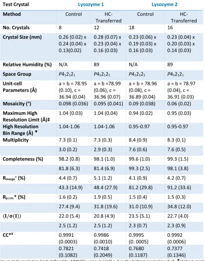
2.3 Average data collection statistics for lysozyme 59
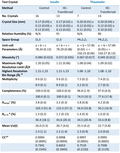
2.4 Average data collection statistics for insulin and thaumatin 63
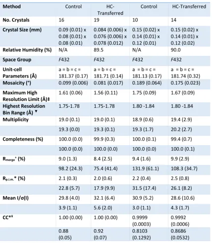
2.5 Average data collection statistics for ferritin 66
2.6 Mann-Whitney U-test results for lysozyme, thaumatin, insulin and ferritin populations
68
2.7 Student’s t-test results for lysozyme, thaumatin, insulin and ferritin populations
68
2.A1 Correlation coefficients for lysozyme, thaumatin, insulin and ferritin populations
77
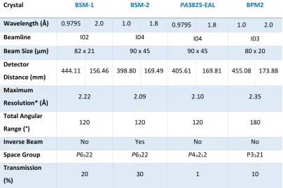
3.1 Data Collection parameters for bacteriocin syringacin M, PA3825-EAL and bacteriocin pectocin M2
85
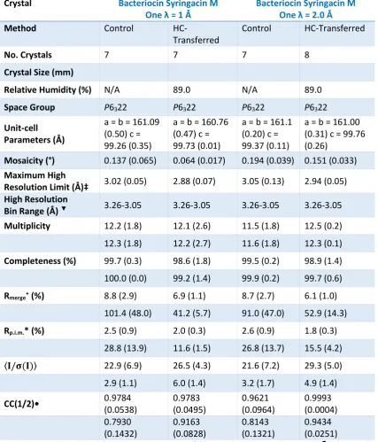
3.2 Average data collection statistics for bacteriocin syringacin M-one, control vs HC-T
91
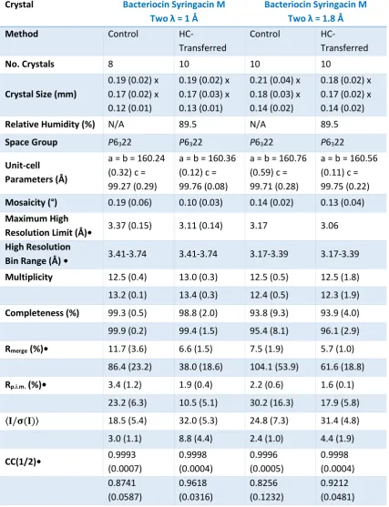
3.3 Average data collection statistics for bacteriocin syringacin M-two, control vs HC-T
93
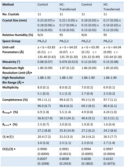
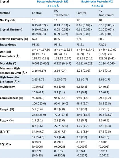
3.4 Average data collection statistics for PA3825-EAL control vs HC-T 97 3.5 Average data collection statistics for bacteriocin pectocin M2, control vs HC-T 101 3.6 Student’s t-test results for bacteriocin syringacin M, PA3825-EAL and
bacteriocin pectocin M2, control vs HC-T
104
3.7 Average data collection statistics for bacteriocin syringacin M-one, like vs like 107 3.8 Average data collection statistics for bacteriocin syringacin M-two, like vs like 111 3.9 Average data collection statistics for bacteriocin pectocin M2, like vs like 114 3.10 Student’s t-test results for bacteriocin syringacin M and bacteriocin pectocin
M2, like vs like
115
3.A1 Flux measurements at 10% transmission 127
3.A2 RADDOSE-3D input parameters 127
3.A3 Normality tests results for bacteriocin syringacin M, PA3825-EAL and bacteriocin pectocin M2 at 1 Å
128
3.A4 Normality tests results for bacteriocin syringacin M, PA3825-EAL and bacteriocin pectocin M2 at 2 Å
129
5.1 AxUDT data collection parameters 166
2
5.3 AxABH data collection and refinement statistics 177
5.A1 AxUDT S-SAD crystal forms 184
6.1 PA3825-EAL data collection parameters 211
6.2 PA3825-EAL data collection and refinement statistics 221
6.3 EAL domains in the PDB 232
6.A1 MucR-EAL data collection and refinement statistics 235
7.A1 AcNiR data collection and refinement statistics for dataset 1-11 288 7.A2 AcNiR data collection and refinement statistics for dataset 12-16 289 7.A3 AcNiR data collection and refinement statistics for dataset 17-40 290 7.A4 AcNiR T1Cu bond distances and angles for dataset 1-14 291 7.A5 AcNiR T1Cu bond distances and angles for dataset 15-40 291
7.A6 AcNiR T2Cu bond distances for datasets 1-13 292
3
Figures
1.1 Bragg’s Law 16
1.2 The Ewald sphere 17
1.3 The Fourier cat and duck 23
1.4 Breaking Friedel’s law 26
1.5 SAD phasing ambiguity 28
2.1 The capillary-top mounting system 35
2.2 The crystal catcher 36
2.3 Graphene mounting 37
2.4
Pulsed UV laser soft ablation Crystal shaping
372.5 CrystalDirect 39
2.6 The Free-mounting system 40
2.7 The HC1 humidity control device 41
2.8 Lysozyme, thaumatin, insulin and ferritin crystals 44
2.9 The crystal transfer apparatus fishing and transfer microscope 47
2.10 The crystal transfer stage 48
2.11 The crystal transfer stage, close up 49
2.12 Stepwise transfer of protein crystals 51
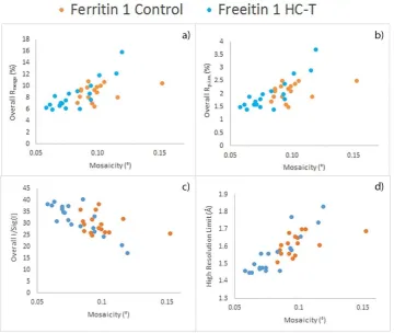
2.13 Graph of individual lysozyme 1 data quality indicators, control vs HC-T 57 2.14 Graph of individual lysozyme 2 data quality indicators, control vs HC-T 58 2.15 Graph of individual insulin data quality indicators, control vs HC-T 60 2.16 Graph of individual thaumatin data quality indicators, control vs HC-T 62 2.17 Graph of individual ferritin 1 data quality indicators, control vs HC-T 64 2.18 Graph of individual ferritin 2 data quality indicators, control vs HC-T 65 2.19 Graph of average data quality indicators for lysozyme, thaumatin, insulin and
ferritin
4
3.1 The Structure of bacteriocin syringacin M 81
3.2 The Structure of bacteriocin pectocin M2 82
3.3 Crystal packing of bacteriocin syringacin M and bacteriocin pectocin M2 83 3.4 Control and HC-transferred bacteriocin syringacin M, PA3825-EAL and
bacteriocin pectocin M2
84
3.5 Measured photon flux on Diamond Light Source beamline I04 86 3.6 Bacteriocin pectocin M2 crystal orientations and dose isosurface 87 3.7 Graph of individual bacteriocin syringacin M-1 data quality indicators, control
vs HC-T
92
3.8 Graph of individual bacteriocin syringacin M-2 data quality indicators, control vs HC-T
94
3.9 RADDOSE-3D analysis graphs for bacteriocin syringacin M 95 3.10 Graph of individual PA3825-EAL data quality indicators, control vs HC-T 98
3.11 RADDOSE-3D analysis graphs for PA3825-EAL 99
3.12 Graph of individual bacteriocin pectocin M2 data quality indicators, control vs HC-T
102
3.13 RADDOSE-3D analysis graphs for bacteriocin pectocin M2 103 3.14 Graph of average data quality indicators for bacteriocin syringacin M,
PA3825-EAL and bacteriocin pectocin M2, control vs HC-transferred
105
3.15 Graph of individual bacteriocin syringacin M-1 data quality indicators, like Vs like
108
3.16 Graph of individual bacteriocin syringacin M-2 data quality indicators, like Vs like
110
3.17 Graph of individual bacteriocin pectocin M2 data quality indicators, like Vs like 113 3.18 Graph of average data quality indicators for bacteriocin syringacin M,
PA3825-EAL and bacteriocin pectocin M2, like vs like
116
3.19 Photo-bleaching of bacteriocin pectocin M2 122
5
4.1 The hallmarks of cancer 132
4.2 The oncogenic mechanisms of CIP2A expression 134
4.3 Myc stabilisation by CIP2A 136
4.4 Akt protein targets 137
4.5 The structure of PP2A 138
4.6 The PP2A network 140
4.7 pET-28 b (+) vector map 142
4.8 CIP2A predicted domain structure 144
4.9 CIP2A N-terminal molecular modelling 146
4.10 CIP2A N-terminal predicted binding sites 147
4.11 SDS-PAGE of CIP2A expression trials 149
4.12 SDS-PAGE of CIP2A Ni-affinity purification 150
4.13 CIP2A Ni-affinity elution chromatograph 151
4.14 SDS-PAGE of CIP2A solubility tests 152
4.15 SDS-PAGE of CIP2A gel filtration purification 152
4.16 CIP2A gel filtration chromatograph 153
4.A1 CIP2A BLASTp sequence alignment 156
4.A2 PSIPRED secondary structure prediction 157
4.A3 FFPred secondary structure prediction 158
5.1 A schematic diagram of the α/β hydrolase fold 162
5.2 pET-47 b (+) vector map 164
5.3 SDS-PAGE of AxUDT and AxABH expression trails 169
5.4 SDS-PAGE of AxUDT Ni-affinity purification 169
5.5 SDS-PAGE of AxUDT Gel filtration purification 169
5.6 AxUDT gel filtration chromatograph 170
6
5.8 AxABH gel filtration chromatograph 171
5.9 AxUDT ammonium sulphate and PEG 3350 crystals 172
5.10 AxABH PEG 3350 crystals 174
5.11 The crystal structure of AxABH 178
5.12 AxABH BIS-Tris ligand binding 179
5.13 AxABH crystal forms 180
5.14 AxABH crystal form superposition 181
5.15 AxABH active site superposition 182
5.16 AxABH active site ligand conformations 183
6.1 Bacterial species cultured from cystic fibrosis sufferers 187
6.2 The degradation and synthesis of cyclic di-GMP 193
6.3 The structure of GGDEF-domains 196
6.4 GGDEF domain regulation by dimerisation, PleD 198
6.5 GGDEF domain regulation by dimerisation, WspR 198
6.6 HD-GYP active site structure 200
6.7 The crystal structure of PmGH 201
6.8 Superposition of open and closed HD-GYP domains 202
6.9 HD-GYP and EAL domain cyclic di-GMP binding 203
6.10 The metal coordinating residues of EAL doamins 203
6.11 Cyclic di-GMP bound Blrp1 active site 204
6.12 Regulation of EAL-domain activity by inter-metal distance 206
6.13 PA3825-EAL initial crystal hits 207
6.14 FPLC chromatographs of EAL domain activity over a range of pHs 210
6.15 PA3825-EAL domain catalytic rates 214
6.16 Chromatograph of minimum detectable cyclic di-GMP 215
7
6.18 PA3825-EAL size exclusion chromatography coupled with multi angle light scattering chromatographs
217
6.19 Monoclinic and tetragonal PA3825-EAL dimerisation interfaces 218 6.20 The Crystal structure of PA3825-EAL and ligand density 219
6.21 Β-sheet conformational changes 222
6.22 Activating loop conformational changes 223
6.23 PA3825-EAL cyclic di-GMP bound active site with Mg2+ and Ca2+ 224 6.24 Inter-metal distances of bimetallic EAL domains in the PDB 226 6.25 Hexagonal and tetragonal PA3825-EAL dimerisation interfaces 228
6.26 The M3 metal binding site 229
6.27 FimX-EAL pGpG binding 231
6.28 Superposition of pGpG bound EAL domains 233
6.29 Superposition of cyclic di-GMP and pGpG bound PA3825-EAL, CC3396-EAL and FimX-EAL
234
6.30 The crystal structure of MucR-EAL 235
6.31 Cyclic di-GMP bound MucR-EAL active site 236
6.32 Superposition of PA3825-EAL and MucR-EAL dimers 238
6.33 Sequence alignment and superposition of H8 dimerisation helix 240
7.1 The reaction of the nitrogen cycle 245
7.2 The conserved structure of copper nitrite reductases 247
7.3 Type-2 copper liganding residues 250
7.4 SDS-PAGE of AcNiR ammonium sulphate precipitation purification 260
7.5 AcNiR crystals 261
7.6 Serial data collection data quality graphs 262
7.7 Nitrite modelling options (dataset one) 264
7.8 Nitrite modelling options (dataset eleven) 265
8
7.10 AcNiR reaction movie 269
7.11 Close up of nitrite and nitric oxide electron density 270
7.12 Nitric oxide modelling options 273
7.13 Superposition of type-one and type-two copper ligands 277
7.14 AcNiR water channel 278
7.15 AcNiR water chain movie 279
7.16 AcNiR water chain superposition with atomic resolution AcNiR 283 7.17 Superposition of nitrite reductase water chains from various species 284
9
Abbreviations
ABH α/β hydrolase
Ac Achromobacter cycloclastes
AcNiR Achromobacter cycloclastes nitrite reductase APC Adenomatous polyposis coli
Arm Armadillo repeat
Ax Achromobacter xylosoxidans
AxABH Achromobacter xylosoxidans α/β hydrolase
AxUDT Achromobacter xylosoxidans UTP-glucose-1-phosphate uridyltransferase bdlA Biofilm dispersion locus
BLAST Basic Local Alignment Search Tool BLUF Blue-light using FAD
BPM2 Bacteriocin pectocin M2 BSM Bacteriocin syringacin M
cd1-NiR Cytochrome cd1 nitrite reductase CDC Centre for disease control
CdG Cyclic di-GMP
CIP2A Cancerous inhibitor of protein phosphatase 2A CIP2A-C CIP2A C-terminal domain
CIP2A-N CIP2A N-terminal domain CUP Chaperone/usher protein
CV Column volume
DGC Diguanylate cyclase
DUF Domain of unknown function FAP Functional amyloids in Pseudomonas
FMS Free-mounting system
10 HC1 Humidity control device
HC-T Humidity control transferred HEWL Hen egg white lysozyme HRL High resolution limit HTH Helix turn helix IP (site) Primary inhibition site keV Kilo-electron volts
MAD Multi-wavelength anomalous dispersion MALS Multi-angle light scattering
MBP Maltose binding protein
MGy Mega grey
MIR Multiple isomorphous replacement
MR Molecular replacement
MX Macromolecular crystallography
PDB Protein data bank
NLS Nuclear localisation sequence PAD PP2A activating drug
PDE Phosphodiesterase
PEEK polyetheretherketone PEG Polyethylene glycol
pGpG 5’- Phosphoguanylyl- (3’ −> 5’)- guanosine PP2A Protein phosphatase 2A
PULSA
Pulsed UV laser soft ablation
Rmease
Redundancy independent merging factor
RmergeLinear merging factor
11
S-SAD
Sulphur single-wavelength anomalous dispersion
SDS-PAGE Sodium dodecyl sulphate polyacrylamide agarose gel electrophoresis SEC Size exclusion chromatography
siRNA Small interfering RNA
SUMO Small ubiquitin-related modifier
T1Cu Type one copper
T2Cu Type two copper
TIM Triosephosphate isomerase UTR Untranslated region
12
Acknowledgements
I would like to thank the following;
My supervisors Dr Richard Strange, Dr Armin Wagner and Prof. Samar Hasnain for their
support, guidance, patience and advice throughout my studies.
Dr Domenico Bellini for all lessons in high throughput protein production and crystallisation.
As well as occasional trips to the pub.
The I23 team, particularly Dr Ramona Duman for all her help with the HC1 project and Dr
Vitaly Mykhaylyk for always making Friday meetings more interesting.
Dr Svetlana Antonyuk for her advice on all things AcNiR.
The staff of the Diamond Light Source and Research Complex at Harwell for providing and
maintaining excellent facilities for scientific research during my stay. Particularly Dr Juan
Sanchez-Weatherby for help with the HC1 and Maria Rosa for maintaining the labs and
making many litres of media for me.
Dr Rhys Grinter for providing protein samples for HC1 tests.
The students of the Molecular Biophysics group and the members of the Oxford Ultimate
Club for the lighter side of life.
The BBSRC and Diamond Light Source for providing a 4 year PhD studentship award
supporting me through the course of my studies.
13
Preface
This Thesis presents original research carried out by the author submitted in accordance with the requirements of the University of Liverpool for the degree of Doctor in Philosophy to the University of Liverpool
This research consists of a number of studies using X-ray crystallography to (1) assess the effects of humid air streams, sample handling and excess surrounding solvent on data quality in long wavelength data collection using robust statistical analysis; (2) produce protein crystals with a view to perform in-vacuum S-SAD phasing experiments; (3) investigate the structure of a novel α/β hydrolase enzyme from the Alcaligenes xylosoxidans genome; (4) better understand the regulation of cyclic di-GMP cleavage by PA3825-EAL and other EAL domain containing proteins and (5) to develop the use of fast detectors and automatic processing pipelines for serial data collection of metallo-proteins to analyse their reaction mechanisms and produce structural movies.
14
15
1.1. Introduction
X-ray crystallography is the premier technique for obtaining three dimensional structural information for chemical and biological molecules. The method involves measurement of the intensity of X-rays diffracted by a crystal made up of a regular repeating lattice of macromolecules or other small molecules. There are several textbooks that cover the principles of X-ray diffraction (Glusker and Trueblood, 1985; Blundell and Johnson, 1976; Blow, 2002 and Rupp, 2010) so will only be discussed briefly here.
When X-rays are scattered by electrons they are either scattered elastically, with no energy loss and X-ray photons are emitted at the same frequency as it entered, or inelastically, where electrons accept some energy from incoming X-ray photon reducing the energy of the emitted photon. When X-rays diffract from a crystal the contribution of the molecules in the regular lattice amplifies the signal you would see from a single molecule to produce discrete diffraction spots. Using Bragg’s law (equation 1.1) we can quantify the angle at which X-rays are scattered (θ) relative to the distance between points in the crystal lattice (dhkl), as shown in Figure 1.1 where X-rays are seen to be reflected from a set of planes in a crystal.
𝑛𝜆 = 2𝑑ℎ𝑘𝑙sin 𝜃
(1.1)
16
Analysis of X-rays scattered by electrons allows us to calculate how the electrons are distributed through a crystal using the electron density equation, which expresses electron density at any point (x,y,z) in the unit cell as a Fourier series; a representation of a function as the sum of sine wave.
𝜌(𝑥, 𝑦, 𝑧) = 1
𝑉∑ ∑ ∑ 𝐹(ℎ𝑘𝑙) exp(−2𝜋𝑖(ℎ𝑥 + 𝑘𝑦 + 𝑙𝑧))
𝑙 𝑘 ℎ
(1.2)
The structure factors F(hkl) represent the information obtained through the crystallographic experiment which is defined as,
𝐹(ℎ𝑘𝑙) = ∑ 𝑓𝑗exp (2𝜋𝑖(ℎ𝑥𝑗+ 𝑘𝑦𝑗+ 𝑙𝑧𝑗)) 𝑁
𝑗=1
17
where V represents the volume of the unit cell, h, k, and l represent the Miller indices (reciprocal index vectors representing 3D crystallographic lattice planes) of any particular reflection, xj, yj and zj represent the coordinates of the jth atom and fj is the scattering factor of the jth atom. The structure factors can be simplified to,
18
where Fhkl represents the measured amplitude obtained during crystallographic experiments as intensities and αhkl is the phase of the structure factor for all measured reflections which must be determined mathematically to “solve” the structure of the crystallised molecule.
1.2. Data Collection
Diffraction data for all test crystals and structures solved in this thesis were collected at Diamond Light Source, UK, on beamlines I02, I03, I04, I04-1 and I24 on Dectris Pilatus 6M detectors. All data were collected using fine phi data collection strategies to minimise the contribution of background noise, allow 3D profile fitting of partial observations to reconstruct full reflections and reduce overlap in reflections from intersecting lunes (Mueller et al., 2012). To determine the amount of data required for a complete dataset the space group of the macromolecular crystal must be determined.
1.3. Space Groups
Space groups represent a group of mathematical symmetry opperations including translational, rotational (two-, three-, four- and six-fold operation) and translational-rotational operations (screw-axes and glide planes). Translation opperations result in fourteen Bravais lattices which give 230 unique space groups when combined with up to three other symmetry opperators. Due to the chirality of proteins and the need to maintain handedness in protein crystals, mirror planes, glide planes, improper rotations and inversion opperations are not allowed; leaving 65 chrial space groups in MX.
19
correctly identify the anantiomorph of these space groups an atomic position is required to fix the origin. Crystal structures may need to be reindexed if processed in the wrong anantiomorph.
1.4. Data reduction
Data reduction is a two-step process consisting of, (1) indexing diffraction spots to assign consistent unit cell vectors (h,k,l) to the diffraction pattern and (2) calculating reflection intensities. All data in this thesis were processed with XDS. XDS uses a robust auto-indexing system which derives reciprocal cell axis lengths from difference vectors between pairs of neighbouring reciprocal lattice vectors to produce a “reduced cell” in P1 and the lattice is fitted to the strongest 3000 reflections (Kabsch, 2010b, Kabsch, 2010a). The lattice is then refined against the strongest 3000 reflections followed by all found reflections and the Bravais lattice is calculated and fitted to possible space groups.
Integration involves accurate measurement of reflection intensities over multiple frames as all data collected in this thesis were collected using fine phi slicing so only partial reflections were recorded. XDS first calculates the frames and pixel positions which contribute to each reflection and generates a coordinate system. An average profile of strong reflections is then generated and the intensity is estimated by determining the background level and generating 3D profiles of contributing pixels for each reflection (Kabsch, 2010b, Kabsch, 2010a).
Individual images are then scaled to account for variations in the intensity of the beam, the illuminated crystal volume, absorption of the beam, radiation damage, detector sensitivity and differences in crystal size/order when scaling multiple crystals (Kabsch, 2010a). Correction factors are defined by,
𝛹ℎ𝑙= (𝐼ℎ𝑙− 𝑔𝑙𝐺𝑙𝐼ℎ)/𝜎ℎ𝑙
20
where h represents a unique reflection, hl represents symmetry-related reflections to h that are corrected by the reciprocal scaling factor gl. Ihl is the reflection’s and symmetry related reflection’s weighted mean and σhl their standard deviation. Ih represents the “true” intensities as defined in detail in Kabsch (2010a). Finally data are merged into a single dataset and structure factors are calculated.
1.5. Data Quality
A number of metrics are applied to merged diffraction data to determine the relative error between measured reflections in individual resolution shells and the overall dataset. The signal-to-noise ratio, commonly referred to as the I/σ(I) is defined as,
|𝐼| 𝜎(𝐼)=
1
𝑁∑
𝐼(ℎ) 𝜎(𝐼(ℎ)) 𝑁
ℎ (1.6)
21
𝑅𝑚𝑒𝑎𝑠 = ∑ ( 𝑁𝑁 − 1)
1 2
∑𝑁 |𝐼(𝑖ℎ)− 𝐼̅(ℎ)|
𝑖=1 ℎ
∑ ∑𝑁 𝐼(𝑖ℎ)
𝑖=1 ℎ (1.7)
where h is any given reflection, Ih is the intensity of an individual reflection, 𝐼̅(ℎ) is the average intensity of symmetry related reflections and N is the total number of reflections in the defined
resolution bin. The precision-indicating merging factor (Rp.i.m.), which adds (𝑁−11 )
1 2
to the summation of reflection in the Rmerge function in a similar vein to Rmeas, has also been adopted as it shows increasing precision of intensity measurements with increasing redundancy (Weiss and Hilgenfeld, 1997, Weiss, 2001).
Another indicator becoming more common place is the use of correlation coefficients as a measure of data quality and maximum high resolution limit. Unmerged data is separated into two randomly selected half sets of unique reflections and calculate the correlation coefficient between averages half sets to give the CC1/2 (Karplus and Diederichs, 2012). The correlation between the CC1/2 and the CCtrue (the correlation of the averaged dataset with noise-free true signal), CC*, is calculated by,
𝐶𝐶∗= √ 2𝐶𝐶1/2
1 + 𝐶𝐶1/2
(1.8)
1.6. Phasing
22
combining the magnitude from the Fourier transform of a duck (Fig. 1.3a) with the phase from the Fourier transform of a cat (Fig.1.3b) results in reconstruction of the image of the cat (Fig. 1.3c). There are several different methods that have been developed for determination of phases for macromolecular structures. The first used being multiple isomorphous replacement (MIR) by Perutz on the structure of haemoglobin using two bound mercury atoms (Green et al., 1954).
1.6.1. Multiple Isomorphous Replacement
24
1.6.2. Molecular Replacement
Molecular replacement (MR) involves the use of a known homologous structure, preferably with 30% or higher sequence identity and similar secondary structure, to determine the initial phases for an unknown structure. As of 2010 structures solved by MR account for over 95% of structures in the PDB (Vagin and Teplyakov, 2010b). Six parameters are applied to homologous structures, a 3D rotation search and a 3D translation search, to position the known structure on top of the unknown crystal structure and calculate initial phases. MR depends heavily on the Patterson function, which is used to calculate a vector map of a structure through a Fourier transform of intensities and amplitudes with a phase of zero. These maps represent the interatomic vectors of the structure which can be used to orientate a model in the unit cell of the unknown crystal structure. The self-Patterson of a known structure can be calculated in any orientation (rotation) and compared with the self-Patterson of the unknown structure. When these self-Pattersons match, the correct orientation of intramolecular parts of the structure have been determined and the fit is measured with the cross rotation function developed by Rossmann and Blow (1962),
𝑅 = ∫ 𝑃2(𝑋2)𝑃1(𝑋1) 𝑑𝑥1 𝑈
(1.9)
25
1.6.3. Phasing With Anomalous Signal
Much like the differences introduced into the diffraction pattern and Patterson map in multiple isomorphous replacement, anomalous signal can be utilised in a similar manner by altering the atomic scattering factor. The atomic scattering factor consists of three terms, (1) the normal scattering term (f0) which is dependent on the Bragg angle; (2) the dispersive term (f’) which affects the normal scattering factor and (3) the absorption term (f”) which causes a phase change of +90°. Both f’ and f” contribute to the anomalous scattering factor and are wavelength dependent; appearing at the absorption edge of an element when an electrons is ejected from a lower shell leaving a space for higher shell electrons to fill. Descending electrons produce X-ray emissions specific to absorbing elements which is measured as anomalous signal (Taylor, 2010).
𝑓(𝑺,𝜆) = 𝑓(𝑠)0 + 𝑓(𝜆)′ + 𝑖𝑓(𝜆)"
(1.10)
The presence of this anomalous signal causes a breakdown in Friedel’s law (|Fhkl| = |F-h-k-l|) as shown in Figure 1.4. Without anomalous signal Friedel’s law holds with the sum of all normal and anomalous scattering atoms (FPA and F-PA) being symmetrical over the real axis (Fig. 1.4a). In the
presence of anomalous signal (FA) the combination of the dispersive term (green) and absorption
term (purple) (Fig. 1.4b) cause a significant difference between FPA and F-PA (dark blue) over the real
26
1.6.4. MAD Phasing
27
and gives a non-native representation of the protein which may affect interpretation of the biological function.
1.6.5. SAD Phasing
The first demonstration of single-wavelength anomalous dispersion (SAD) phasing was the structure of crambin by Hendrickson and Teeter (1981) using six native sulphur atoms. SAD experiments measure the differences in intensity between a Bijvoet pair (Eqn. 1.11) from a single crystal collected above or at an energy above an absorption edge.
∆𝐹±= |𝐹
𝑃𝐻(+)| − |𝐹𝑃𝐻(−)| (1.11)
28
1.6.6. Long Wavelength MX for Sulphur-SAD
29
signal that can be obtained from native sulphurs in a protein crystal at different X-ray energies can be determined using the Bijvoet ratio,
𝐵𝑅 = (𝑁𝐴 2𝑁𝑇)
1 2
(2𝑓"𝐴 𝑍𝑒𝑓𝑓) (1.12)
where NA is the number of anomalous scatterers in the unit cell, NT is the total number of atoms in the unit cell, f” is the anomalous scattering factor at a set energy and Zeff is the normal scattering power (6.7 e- at 2θ = 0). It has been suggested that a Bijvoet ratio of at least 0.6% is necessary for successful phasing by SAD (Wang, 1985). Although use of longer wavelength (1.5-3 Å) and long wavelength (>3 Å) X-rays have the advantage of increased anomalous signal for lighter atoms such as sulphur, phosphorous, calcium and chlorine there are several downsides that must be taken into account.
30
improved over the years, standard MX beamlines are unable to use long wavelength X-rays to their full potential due to absorption and scattering of X-rays in air, absorption in the crystal and the larger diffraction angles from the X-rays (Djinovic Carugo et al., 2005). In an attempt to harness the power of long wavelength X-rays, Diamond Light Source have developed the first in vacuum beamline for long wavelength MX, I23.
1.7. I23 – In-vacuum MX
To reduce the effects of background noise on the detector from air scatter as well as the absorption of the X-ray beam in air I23 has been designed to operate in vacuum, with the entire experimental setup in a large vacuum chamber. By performing diffraction experiments in vacuum scattering of X-rays by air is eliminated, leaving only background scatter from the crystal and sample mount. The signal-to-noise ratio can also be improved by removing non-crystalline solvent surrounding the crystal which causes water rings to appear on the diffraction image. Chapters Two and Three of this thesis deal with the effects of longer wavelength X-rays in the presence and absence of excess surrounding solvent on data quality. Performing diffraction experiments in vacuum means conventional cooling of protein crystals with a stream of liquid nitrogen is not possible so I23 has adopted a conductive cooling mechanism. Extensive work has been carried out on the viability of cooling by conductance through the goniometer and specially designed sample mounts (Warren et al., 2013). Cooling by conductance also has the added benefit of minimising sample vibrations from the cryo-stream which can have a negative effect on the signal-to-noise ratio (Alkire et al., 2008, Alkire et al., 2013). Finally, with respect to improving signal-to-noise, a semi-cylindrical Pilatus 12M detector has been designed to allow rapid data collections with minimal readout noise and to account for the large scattering angles from long wavelength X-rays.
31
most absorption correction programs use a rough estimation of crystal volume. I23 will employ an X-ray tomography system to allow accurate measurement of the crystal volume post data collection for more accurate absorption correction. Tomographic reconstruction of macromolecular crystals has been demonstrated by Brockhauser et al. (2008) on lysozyme and DNA crystals. X-ray tomography has also been used as a low dose alternative to the grid scans for location of small membrane protein crystals cooled in opaque lipidic cubic phase mother liquor (Warren et al., 2013).
32
Chapter 2 – Sample Preparation for Long
33
2.1. Introduction
As modern macromolecular crystallography (MX) is used to tackle more and more
difficult projects, there is a pressing need to improve the quality of diffraction data.
Development of synchrotron instrumentation has greatly improved the reliability, accuracy
and speed of data collection to the point that sample quality is becoming the more
significant stumbling block. The major limiting factors affecting diffraction data include
crystal quality, radiation damage and the signal-to-noise ratio. Improving crystal quality
requires the systematic optimisation of crystallisation conditions and cryo-protection which
can be very time consuming and may require rescreening to find alternative crystallisation
conditions. Radiation damage results from interactions of the X-ray beam with the electrons
in the crystal. Although X-ray diffraction is an elastic process, X-ray absorption and Compton
scattering deposit energy in crystals, causing damage and a reduction in diffracting power
(Teng and Moffat, 2000, Garman and Weik, 2015). These effects are wavelength dependent
at typical MX energies (12.4 keV), with damage proportional to absorbed X-ray dose (Owen
et al., 2006a, Murray et al., 2005, Henderson, 1990). The development of X-FEL technology
allows a “collect-before-destroy” approach to overcome the effects of primary radiation
damage caused by direct interaction of X-ray radiation with electrons to break chemical
bonds (Neutze et al., 2000, Teng and Moffat, 2000). However, access to X-FELs is very
limited so does not present a feasible alternative to synchrotron radiation for the MX
community. Secondary damage results from chemical reactions of highly reactive species
produced by ionising radiation, such as hydroxyl radicals, hydrated electrons and H atoms
(Burmeister, 2000, Teng and Moffat, 2000, Garman, 2003a, Murray et al., 2004, Owen et al.,
34
data collection performed at cryo temperatures (Hope et al., 1989) or by outrunning
damage with fast detectors and very short exposure times (Owen et al., 2014a).
Maximising the signal-to-noise ratio has been addressed through improved data
collection techniques, largely enabled by modern synchrotron instrumentation such as pixel
array detectors (Broennimann et al., 2006a) and microfocus beams (Evans et al., 2007). The
combination of the fine φ-slicing method (Mueller et al., 2012)
and precise targeting with
microbeams (Sanishvili et al., 2008) have both contributed to a significant reduction in
background scatter from surrounding solvent and sample mounts. In addition to exploiting
these advances in synchrotron technology, careful sample preparation can go a long way
towards improving the signal-to-noise ratio during diffraction experiments.
The principal causes of background scatter are the excess solvent around frozen
crystals and the sample mounts. Although this background scatter is not usually considered
a critical issue in standard MX experiments, for the long wavelength experiments required
for accurate phasing and in microcrystal MX, where signals are significantly weaker,
background scatter becomes a limiting factor. As a result, in an effort to improve the signal
to noise ratio, a variety of sample handling techniques have been developed as alternatives
to traditional nylon and Kapton mounts.
The “capillary-top mounting” or “loopless method” was developed to exploit the
use of Cr Κα radiation (2.29 Å) and reduced background scatter to measure the weak signals
associated with S-SAD phasing (Kitago et al., 2005b, Watanabe et al., 2006, Kitago et al.,
2010b). Capillary mounts with removable nylon loops (Fig. 2.1c-d) were incorporated into a
semi-automated setup, which removes surrounding solvent by aspiration and flash freezes
35
method has seen some success in structure solution by S-SAD and presents a good case for
phasing by in-house Cr Κα radiation (Watanabe et al., 2006).
Another technique designed to improve the signal-to-noise ratio is the Crystal
Catcher, designed by Kitatani et al. (2008b) and further tested by Mazzorana et al. (2014).
The Crystal Catcher allows loop free mounting of crystals on an adhesive ejected from a
quasi-SPINE standard pin using a mechanical pencil type mechanism (Fig. 2.2) (Kitatani et al.,
36
Wierman et al. (2013) have also developed a technique using atomically thin
graphene sheets to coat protein crystals. Crystals are wrapped by pipetting crystals into a
drop with a graphene sheet floating at the water air interface of the drop (Fig. 2.3a). As the
crystal floats to the bottom of the drop a nylon loop is used to position the crystal in the
graphene sheet which wraps around the crystal as it is pulled from the drop (Fig. 2.3b)
38
The use of lasers has also been explored for sample preparation in an effort to
increase the signal to noise ratio. Pulsed UV laser soft ablation (PULSA) has been used on
crystals of soluble protein to cut and shape crystals, minimising surrounding solvent without
damaging the structure of the crystal (Kitano et al., 2004, Kitano et al., 2005a, Watanabe et
al., 2006). The technique has been extended to processing of membrane proteins and the
removal of nylon loops using PULSA (Kitano et al., 2005b). CrystalDirect (Cipriani et al.,
2012) also employs laser-induced photoablation for sample preparation with a femtosecond
laser used to excise protein crystals grown on ultrathin films. This technique aims to
completely automate crystal harvesting and reduce background scatter in the process (Fig.
2.5) (Cipriani et al., 2012). The work by Cipriani et al. (2012) corroborates the findings that
the use of PULSA has no detrimental effects of crystal quality.
Although not originally designed for the purpose of reducing background scatter to
improve the signal-to-noise ratio, both the free mounting system (FMS) (Kiefersauer et al.,
1996, Kiefersauer et al., 2000) and humidity controlled device (HC1) (Sanchez-Weatherby et
al., 2009a) allow removal of excess surrounding solvent while maintaining protein crystals in
a humid air stream. Both were designed to exploit the dynamic nature of protein crystals by
using dehydration to alter crystal packing and improve the diffraction power of crystals;
with an ever growing list of success stories (Russo Krauss et al., 2012, Deng et al., 2012,
Newman, 2006, Bowler et al., 2006b, Heras et al., 2003, Heras and Martin, 2005, Kalinin et
al., 2005). The FMS removes a crystal from a nylon loop using a micropipette; the crystal is
maintained within a stream of humid air to allow online dehydration experiments (Fig. 2.6).
The relative humidity of the air stream is regulated by mixing two air streams of 0 and 100%
39
fashion to the capillary top mounting
method. Although the FMS has been
successful in many cases, it has proven
difficult
to
routinely
or
easily
incorporate its bulk into the crowded
synchrotron beamline environment.
This has led to the development
of a more suitable online device, the
HC1, which uses a nozzle based on
standard cryostream technology for
delivery of the humid air stream (Fig.
2.7) (Sanchez-Weatherby et al., 2009a,
Russi et al., 2011). Protein crystals can
be harvested on standard sample
mounts and placed in the humid air
stream, where excess solvent can be
removed to allow more efficient
dehydration (Sanchez-Weatherby et al.,
2009a). The HC1 regulates humidity in a
similar manner to the FMS, using
calculation of the dew point to set the final relative humidity (Kiefersauer et al., 2000).
However, differences arise between the two systems in how the dew point is achieved.
40
2.7b) to cool the incoming air to the calculated temperature and remove excess water
though the condenser (Sanchez-Weatherby et al., 2009a). In this study the HC1 has been
used to maintain protein crystals, as done previously (Sjogren et al., 2002, Sjogren and
Hajdu, 2001b, Sjogren and Hajdu, 2001a), to allow removal of excess surrounding solvent, to
41
All of the studies mentioned above have presented findings based on comparison
of a very small number of (or even just single) protein crystals between treatments, without
validation by an appropriate statistical test (Kitago et al., 2010a, Kitago et al., 2005b, Kitatani
et al., 2008b, Mazzorana et al., 2014, Wierman et al., 2013, Cipriani et al., 2012). However,
studying and accurately evaluating relatively small effects on data quality is very difficult to
achieve due to radiation damage and the intrinsic variability of crystals, even if grown and
42
In this study, a systematic statistical approach was used to determine whether
manual handling and manipulation of crystals in a humidity-controlled stream can be
performed at no cost to the integrity of the sample. To prove this concept, large populations
of macromolecular crystals were transferred between conventional sample mounts, using
micromanipulators to allow precise movement, and the HC1 to preserve the integrity of
macromolecular crystals and enable removal of excess surrounding solvent. crystal transfer
was facilitated by the removal of excess surrounding solvent with a fine paper wick
(Warkentin and Thorne, 2009), giving the added benefits of reduced background scatter and
improved cooling rates during cryo-protection. To assess the effects of manual handling and
the presence of excess solvent, two statistical tests were applied to the crystal/data
populations: Student’s t-test (Student, 1908) and the Mann-Witney-U-test (Mann and
Whitney, 1947). Both tests examine the null hypothesis that the population of transferred
crystals and the population of crystals fished and mounted by conventional methods show
no significant differences in data quality. Initially, experiments during data collection were
conducted at λ = 1 Å, a typical wavelength used in MX, to ensure that sample handling,
exposure to the humid air stream and wicking of excess solvent can be performed at
standard conditions without damaging macromolecular crystals. These experiments and
tests were a precursor and background to testing the effects of excess solvent using long
wavelength data collection (see Chapter 3). At λ = 1 Å it is expected that absorption will be
negligible, so any detrimental effects on data quality will be the result of manual handling
43
2.2. Methods
2.2.1. Protein Crystallisation
Hen egg white lysozyme (HEWL),
porcine
insulin,
Thaumatococcus daniellii
thaumatin and horse-spleen ferritin were selected to study the effects of manipulating
protein crystals and removing excess solvent in a humidity controlled environment. These
proteins are all commercially available, have well defined crystallisation protocols and are
grown in optimised cryo-protection conditions, thus eliminating the additional manual step
of determining cryo-protection conditions, which could introduce random errors into this
systematic study. All proteins were purchased from Sigma-Aldritch (St Louis, Missouri, USA)
and underwent no further purification. Crystals were grown in sitting drops by the vapour
diffusion method at 19°C over several days (Fig. 2.8).
Tetragonal HEWL crystals were grown in 0.8-1.2 M NaCl, 50 mM sodium acetate pH
4.6 and 25% ethylene glycol (v/v) following the protocol by Murray and Garman (2002). 30%
PEG 5K (w/v) was substituted for 25% (v/v) ethylene glycol for cryo-protection.
Porcine
insulin was suspended in 50 mM sodium phosphate with 10 mM EDTA pH 10.2 and
equilibrated against 30% ethylene glycol and 50 mM sodium phosphate with 10 mM EDTA
pH 10.2 in a 1:1 ratio to produce cubic crystals, adapted from the batch method by Meents
et al. (2007). Tetragonal thaumatin crystals were grown by equilibrating 80 mg/ml
thaumatin in 100 mM phosphate buffer pH 6.5 against 30% (w/v) Na/K tartrate, 100 mM
phosphate buffer pH 7 and 20% glycerol, adapted from the modified gel acupuncture
44
M ammonium sulphate, 10 mM cadmium chloride and 25% glycerol (v/v) as detailed by
Murray and Garman (2002).
2.2.2. The Humidity Control Device (HC1)
The main purpose of humidity control devices to date has been to
45
diffraction quality (Sanchez-Weatherby et al., 2009a, Bowler et al., 2006c, Russi et al., 2011).
In my case the HC1 (Arinax, ZI de Centr’Alp, France) was used to (i) maintain protein crystals
in as near a native environment as possible for the physical transfer from one mount to
another and (ii) allow controlled removal of excess surrounding solvent.
2.2.3. Defining Relative Humidity
To prevent protein crystals dissolving, drying out or losing cryo protection when
introduced to the humid air stream their relative humidity must be measured. Relative
humidity was measured by loading a drop of reservoir solution on an empty loop in the
humid air stream and monitoring the change in drop size over time. Too high a relative
humidity causes the drop to grow while too low will cause the drop to shrink. The relative
humidity was adjusted accordingly and the process repeated with a new drop of reservoir
solution until equilibrium was reached and drop size stabilises (Sanchez-Weatherby et al.,
2009a). A fresh drop was used after each humidity adjustment as the concentration of
buffer components may have changed with loss or gain of water from the humid air stream.
All crystal transfer experiments, described later, were carried out under these equilibrium
conditions. The relative humidities of several common crystallisation compounds
have been
measured (Table 2.1) (Wheeler et al., 2012) and these can provide initial relative humidity
targets. However, reservoir solutions with a combination of buffers, salts and PEGs, etc,
were observed to vary considerably from these measured ‘pure’ values (Table 2.1) and
46
Table 2.1: Relative humidity measurements of individual chemicals and crystallisation buffers. All protein crystals reqired no further cryo-protection. For crystals where two populations were produced (lysozyme and ferritin) measured relative humidities are presented as population 1/ population 2.
Individual buffers Relative
Humidity (%) Crystal Buffers
Relative Humidity (%)
0.1 M NaCl 100.00 Ferritin: 0.1 M NaCl, 0.8 M ammonium sulphate, 10 mM cadmium chloride and 25% glycerol (v/v)
89.50/90.00
0.8 M AmSO4 99.25
25% Glycerol
(v/v) 95.00
1.0 M NaCl 99.00 Lysozyme: 0.8-1.2 M
NaCl, 50 mM sodium acetate pH 4.6 and 25% ethylene glycol (v/v)
89.00/89.00 25% Ethylene
Glycol (v/v) 92.00
20% Glycerol
(v/v) 97.00
Thaumatin: 30% Na/K
tartrate (w/v), 100 mM phosphate buffer pH 7 and 20% glycerol
86.00
30% Ethylene
Glycol (v/v) 89.50
Insulin: 30% ethylene glycol and 50 mM sodium phosphate with 10 mM EDTA pH 10.2
91.00
2.2.4. Humidity Control Crystal Transfer Method
In order to genly transfer crystals from one mount to another while removing
excess solvent I constructed and tested the crystal transfer setup (Fig. 2.9), which consists of
two micromanipulator stages, a stationary stage, a light microscope and the HC1.
Macromolecular crystals are transferred from a donor sample mount (Fig. 2.10a) on the
stationary stage (Fig. 2.10b) to an acceptor sample mount loaded with reservoir solution
(Fig. 2.10c) on micromanipulator 1 (Fig. 2.10d). The process is viewed from above using the
47
approximately 1cm from the HC1 nozzle (Fig. 2.10f), within the laminar humid air stream. A
fine paper wick (Fig. 2.10g) attached to micromanipulator 2 (Fig. 2.10h) is used to gently
remove excess solvent.
The step by step transfer is depicted in Figure 2.12. A crystal is harvested from its
drop using the donor mount and placed in the humid air stream opposite the acceptor
mount loaded with reservoir solution (Fig. 2.12a). The acceptor mount is brought into
contact with the donor mount using micromanipulator 1 (Fig. 2.12b) and the excess solvent
removed by wicking (Fig. 2.12c-d). Removing the solvent from the donor mount transfers
48
acceptor mount is then removed from micromanipulator 1 and the crystal flash frozen in the
adjacent dewar of liquid nitrogen (Fig. 2.10i).
Control crystals were harvested directly from their drops using MicroMounts or
LithoLoops and immediately flash frozen in liquid nitrogen. The crystals harvested for
control and HC-transfer were of comparable size for each protein crystal type (Tables 2.3-5).
49
2.2.5. Crystallographic Data Collection and Processing
Crystallographic data were collected over 6 visits on Diamond Light Source
beamlines I03 (lysozyme 1
1, insulin and ferritin 1
1) and I02 (lysozyme 2, thaumatin and
ferritin 2). The total number of individual datasets obtained during all visits for
[control/HC-transferred] crystals were as follows; lysozyme 1 [8/12], lysozyme 2 [18/16], insulin [16/13],
thaumatin [7/14], ferritin 1 [16/19] and ferritin 2 [10/14]. Thus a total of 75 control and 88
HC-transferred crystals were measured on four proteins. All datasets were collected in a
1