Problems in density estimation for independent and dependent data

PROBLEMS IN DENSITY ESTIMATION FOR

INDEPENDENT AND DEPENDENT DATA.

By

Robert Murison

A THESIS SUBMITTED FOR THE DEGREE OF DOCTOR OF PHILOSOPHY

OF

THE AUSTRALIAN NATIONAL UNIVERSITY

CENTRE FOR MATHEMATICS AND ITS APPLICATIONS

© Copyright 1993

I certify that I have read this thesis and that in my opin­ ion it is fully adequate, in scope and in quality, as a dissertation for the degree of Doctor of Philosophy.

l \ ( - v f f c z i /

Professor Peter Hall (Principal Adviser)

I certify that I have read this thesis and that in my opin­ ion it is fully adequate, in scope and in quality, as a dissertation for the degree of Doctor of Philosophy.

rAUirer)________

I certify that I have read this thesis and that in my opin­ ion it is fully adequate, in scope and in quality, as a dissertation for the degree of Doctor of Philosophy.

Dr ^AktirWelsh

Approved for the University Committee on Graduate Studies:

D eclaratio n

I hereby declare that this thesis describes my own original work, supervised by Professor P.G. Hall and published jointly with him.

A ck n o w led gem en ts

I wish to express appreciation and thanks to my supervisor, Professor Peter Hall, for guiding me through the research for this thesis and expanding my statistical horizons.

My research was made possible by the generous financial assistance from Wool Research and Development Corporation and from New South Wales Agriculture. I am very appreciative that both organisations see merit in statistics research and have confidence in me. It will be a pleasure to reciprocate their support in the future.

Dr Andrew Wood was always available and patient to discuss my research and assist me over the hurdles and to him I owe thanks. I also wish a special thanks to my friend and fellow student, Song Xi Chen, for his companionship and moral support as we pursued our research interests.

A s s o c ia te d P a p e r

A b stra ct

The aim of this thesis is to provide two extensions to the theory of nonparametric kernel density estimation that increase the scope of the technique.

The basic ideas of kernel density estimation are not new, having been proposed by Rosenblatt [20] and extended by Parzen [17]. The objective is that for a given set of data, estimates of functions of the distribution of the data such as probability densities are derived without recourse to rigid parametric assumptions and allow the data themselves to be more expressive in the statistical outcome. Thus kernel estimation has captured the imagination of statisticians searching for more flexibility and eager to utilise the computing revolution. The abundance of data and computing power have revealed distributional shapes that are difficult to model by traditional parametric approaches and in this era, the computer intensive technique of kernel estimation can be performed routinely. Also we are aware that computing power can be harnessed to give improved statistical analyses. Thus a lot of modern statistical research involves kernel estimation from complex data sets and our research is concordant with that momentum.

kernel density estimation and we give an outline to our two research topics.

Our first extension to the theory is given in Chapter 2 where we investigate density estimation from independent data, using high order kernel functions. These kernel functions are designed for bias reduction but they have the penalty of yielding negative density estimates where data are sparse. In common practice, the negative estimates would arise in the tails of the density and we provide four ways of correcting this negativity to give bona fide estimates of the probability density. Our theory shows that the effects of these corrections are asymptotically negligible and thus opens the way for the regular use of bias reducing, high order kernel functions.

We also consider density estimation of continuous stationary stochastic processes and this is the content of Chapter 3. With this problem, the dependent nature of the data influences the accuracy of the kernel density estimator and we provide theory regarding the convergence of the kernel estimators of the density and its derivatives to the true functions. An important result from this study is that nonparametric density estimators from dependent processes can have the same rates of convergence as their parametric counterparts yet retain the flexibility of being independent of parametric assumptions. Our other results indicate that the convergence rate of the density estimator can be quite slow if there are large lag dependencies amongst the data and suggests that large samples would be required for reliable inference about such data.

C on ten ts

D e cla r a tio n iv

A c k n o w le d g e m e n ts v

A b stra ct vi

1 I n tr o d u c tio n 1

1.1 The Setting for Kernel Density E stim a tio n ... 1 1.2 Outline of T h e s is ... 2 1.3 Basic Concepts of Kernel Density E s tim a tio n ... 2

2 C o rrectin g th e N e g a tiv ity o f H ig h -O rd er K ern el D e n sity E stim a to r s 6

2.4 Simulation S t u d y ... 25

2.4.1 Simulation Details ... 26

2.4.2 R esults... 28

2.5 Proofs of Results and T heorem s... 41

2.5.1 Proof o f / / 2 = / / 2 + op( l ) ... 41

2.5.2 Proof o f / / 2/ ( / > 0 ) = / / 2 + o „ ( l ) ... 41

2.5.3 Proof of / ( / - / ) / / ( / < 0) < {( ) - ' + 42 2.5.4 Proof o f / ( / - £ / ) / = op{(n/J) - '/ 2} 43 2.5.5 Proof of f (Ef- / ) / = - \ A i h r + ... 44

2.5.6 Proof of Theorem 2 .1 ... 45

2.5.7 Proof of Theorem 2 . 2 ... 56

2.5.8 Proof of Theorem 2.3 ... 61

2.5.9 Proof of Theorem 2.4 ... 62

3 E stim a tio n o f th e D e n sity and M o d e o f a C o n tin u o u s-T im e S ta tio n ­ ary S to c h a stic P r o c e s s 66 3.1 In troduction... 66

3.2 Previous Developments in Density and Mode Estimation for Stationary Processes ... 70

3.2.1 Density E stim a tio n ... 70

3.3 Estimation of the Marginal Density and its Derivatives of a

Continuous-Time P r o c e s s ... 78

3.3.1 The Covariance Function of a Gaussian P r o c e s s ... 79

3.3.2 Kernel Estimators for Continuous-Time Data ... 81

3.3.3 The Bias of ... 82

3.3.4 The Variance of f W ... 83

3.3.5 Asymptotic Variance of f W for Gaussian P ro c e s se s... 84

3.4 Simulation Study of Kernel Density Estimators of a Gaussian Process 95 3.4.1 Generating the Data for a Gaussian P r o c e s s ... 95

3.4.2 Choosing the B an d w id th ... 98

3.4.3 Numerical Study of L2 Convergence of Kernel Estimators . . . 106

3.5 The Surface Roughness D a ta ... 113

3.6 P r o o f s ... 118

3.6.1 Proof of Theorem 3.1... 118

3.6.2 Proof of Theorem 3.2... 134

List of Tables

2.1 Asymptotically optimal kernel functions for r = 2 and r = 4 ... 7 2.2 Values of relative difference (Ri) of /,- for simulated Normal data. . . 33 2.3 Values of relative difference (Rt) of /,• for simulated Cauchy data. . . 34 2.4 Values of relative difference (R{) of /,• for simulated Students’t (2 df.)

data... 35 2.5 Values of relative difference (Ri ) of fi for simulated Students’t (3 df.)

data... 36 2.6 Values of relative difference (Ri) of /,• for simulated Students’t (5 df.)

data... 37 2.7 Values of relative difference (Ri) of /, for simulated Students’t (8 df.)

3.4 Least squares fits of the linear relationship between log(T') and log(/zmin) for different proportions of short and long term dependence... 103 3.5 Least squares fits of the linear relationship between log(T) and log(Ämin)

for different proportions of short and long term dependence... 104 3.6 Comparisons of bandwidths that minimise the ISE and the bandwidths

given by the rules for T = 400 and a = 1 ... 105 3.7 Squared errors for the sample mode of Gaussian processes... 108 3.8 Asymptotic and sample integrated variances (xlO4) of kernel estima­

tors for Gaussian processes of length T=400... I l l 3.9 Asymptotic and sample integrated squared errors (xlO4) of kernel es­

List o f F igu res

2.1 Asymptotically optimal kernel functions for r = 2 and r = 4... 8 2.2 The high-order kernel density estimators / and

f 2

of Normal (0,1), Cauchy (0,1) and Student’s t (2 df) data... 30 2.6 Values of relative difference (ft,) of /, for sample sizes 50,100,200,400,1000

of Student’s t (3 df), Student’s t (5 df) and Student's t (8 df) data. . 31 2.7 Values of relative difference (ft,) of for sample sizes 50,100,200,400,1000

of Gamma(5,l) and Beta(5,9) data... 32 2.8 Ranges fti(e) and ft2(e) of the right tail of / as described in Theorem

2.1... 46 3.1 Line transects of height recordings (Studentised) for new. treated and

3.3 Examples of f ( x ) and f ' ( x ) for simulated continuous-time Gaussian data... 82 3.4 Log-linear relationship between optimal bandwidth and sample size. . 100 3.5 Profiles of sample variances of / and / ' ... 109 3.6 Sample and asymptotic integrated variances of / and / for samples

C h ap ter 1

1.1

T h e S e ttin g for K e rn e l D e n s ity E s tim a tio n

Nonparametric density estimation is established as an important technique of sta­ tistical analysis and whilst it is an effective tool for description of a data set, it is often used as a component of more complex statistical models. The strength of the technique is that it does not require rigid assumptions about the data and is ideally suited to utilise computing power to extract detailed information from the data.

1.2

O utline o f T h esis

We provide statistical theory regarding the correction of negative density estimates that arise from high-order kernels (Chapter 2) and promote the use of kernel density estimators for continuous stationary stochastic processes (Chapter 3).

High-order kernels are well known and practioners often apply ad hoc procedures to correct the negativity. Our theory will provide validity for four useful correction methods. We envisage that this will clear the way for the use of high-order kernels in statistical modelling such as the smoothed bootstrap and generalised additive models.

Our second topic regarding continuous processes is geared for data description at this stage. With large sets of data, we are in a position to extract more information than is achieved by traditional parametric models that use only the first two moments

to summarise the data.

We shall give the basic concepts of kernel density estimation which establish our notation and serve as a reference point for the two topics we consider.

1.3

B asic C on cep ts o f K ernel D en sity E stim ation

The theory we present here is without rigour and is covered in detail by Silver- man [23, Chapter 3].

kernel function K and bandwidth h, the kernel density estimator is

/ ( x ) = ( nh) - 1

Y

,

1 = 1

The kernel function, A'(-), is smooth, continuous, K(t)dt = l(normalization), supx |A"(x)| < oo (bounded) and limp^oo AT(x) = 0. The last condition is easily attained by choosing kernels with compact support. The density estimator, / , will have the same continuity and differentiability properties as K .

The action of K is to smooth the sample probability mass (n-1) associated with each X{ into the neighbourhood within radius h of X{. The choice of h is of funda­ mental importance. If it is too large, the kernel function will oversmooth, obscure the

' h

detail supplied the data and induce excess bias. Conversely, h being too small will undersmooth and the resulting estimator will give too much emphasis to the sample itself and have high variance.

The common approach to choosing a globally optimal bandwidth is to minimise the squared error risk function, integrated over the range of the density. This statistic is known as the mean integrated squared error (MISE) and by the familiar statistical association of bias and variance we have that

MISE = E

J

j

/ + y

sufficient. We shall return to this issue shortly but first we need to consider the effect of the kernel function K.

We shall define K to be and rth order kernel function if

1 if l = 0

0 < l < r

kr ^ 0 / = r

(1.2)

The most straightforward case is when r = 2 but we shall retain the general form since in Chapter 2 we consider those kernel functions where r > 2.

We assume that the unknown density has continuous derivatives of at least order r and that h —► 0, nh —► oo as n —> oo. Then straightforward calculations lead to expressions for the asymptotic bias and variance of /;

bias{/} = (- 1 )ThTf ^ k r/r\ + o(hr) , (1.3)

var{/} = (nh)-1 f

J

Therefore for an rth order kernel we can write

MISE { f ( x ) } ss (nh)-1 J K ( t f d t + 2

j

By differentiating (1.5) with respect to h. or by choosing h so that variance and squared bias are of the same magnitude, we get that

(V2~r kr/r\)-2 U J K( t )

l / ( 2 r + l )

, - l / ( 2 r + l)

(1.6)

to have the same scale and location as the data. Another proposal is to use least- squares cross validation for estimating hopt. This process is attractive since it can be automated and it makes only weak asumptions about / but the resampling involved can introduce extra noise and the chosen bandwidth may be too wide. Silverman [23] explains bandwidth choice by cross-validation and gives references to research on that topic.

Substitution of the result from (1.6) back into the approximate formula for MISE ( (1.5) ) gives that

MISE « 2r + l

2r

T l / ( 2 r + l )

X)} dx ra- W ( w i)

where C( K) = ^ y/2r kT

(1.7) > 2r/ ( 2r + l)

= 0 {„-W O+O} . (1.8)

C h a p te r 2

C o r r e c tin g th e N e g a tiv ity o f

H ig h -O rd e r K e r n e l D e n s ity

2.1

I n tr o d u c tio n

The bias in kernel density estimation arises as we smooth the empirical probability from the sample points into the neighbourhoods surrounding them. The degree of smoothing, and hence bias, is determined by the bandwidth and by the nature of the kernel function. We can see from equation (1.3) that for an rth order kernel, the asymptotic bias has factors of hr/r\ and kr = / trK(t)dt. In the Taylor series expansion for bias (see Silverman [23, pp39]), terms of hl/l\ f tlK( t )dt, 0 < / < r, are zero due to properties (1.2) of K(t) and the bias is 0{hT). Since h -► 0 as n -► oo, larger values of r will give smaller orders of magnitude of bias.

High order kernels (r > 2) were proposed by Parzen [17] and Bartlett [2] as means to reduce the bias of density estimators. If r = 2, K is itself a density function since it integrates to 1 and does not have negative values. For r > 2, K must take some negative values in order that it integrates to 1. This leads to negative density estimates in places where the data are sparse, even though in other places the density estimates profit from the reduced bias.

Inless n is very large, it would seem that only a modest gain may be achieved by choosing a kernel of order greater than 2, given the negative values of / that accompany it. For instance using equation (1.8), with n = 100 and r = 2, the MISE is 0(0.025) and for r = 4, it is 0(0.017). The advantages of high order kernels are found in higher level statistical procedures that use density estimators. Hall, DiCiccio and Romano [13] proved that the estimate of variance of a quantile, derived from bootstrap samples that are smoothed by a r ’th order kernel, have a precise order of error equal to n ~r/(2r+1)> However, bootstrap sampling demands that the density estimate be positive. If the gains of a high order kernel are to be realised, it is necessary to correct the negative values in the tails of / whilst retaining the order of bias for the interior points.

The optimal kernel to minimise the asymptotically optimal MISE is found by min­ imising / K( t ) 2dt subject to the constraints of equation (1.2). A generating function for optimal kernels has been given by Gasser, Muller and Mammitzsch [11] and they list several optimal kernels such as those in Table 2.1.

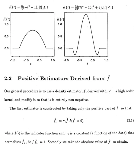
Table 2.1: Asymptotically optimal kernel functions for r = 2 and r = 4 .

r = 2 K(t ) = |( - < 2 + l) _{1*1 < 1}

=0 _{1*1 > 1}

r = 4 K(t ) = if(7 f4 — 10f2 + 3) _{1*1 < 1}

=0 _{1*1 > 1}

Plots of these kernels in Figure 2.1 illustrate how bias is reduced with a high order kernel. With a fourth order kernel function, the density estimate at some data point

Xi. The second order kernel function smooths by using more information from the edges of the smoothing window so that distant points have more influence on the density estimate than is the case with a fourth order kernel function.

Figure 2.1: Asymptotically optimal kernel functions for r = 2 and r = 4.

K(t) = f(-< 2 + 1), |f| < 1 K(t) = |f(7 i4 - 10i2 + 3), |<| < 1

m

1.0

0.5

0.0

-1.5 -0.5 0.5 1.5 -1.5 -0.5 0.5 1.5

t t

A

2.2

P o s itiv e E s tim a to r s D e r iv e d fro m /

Our general procedure is to use a density estimator, / , derived with v* a high order kernel and modify it so that it is entirely non-negative.

The first estimator is constructed by taking only the positive part of / so that,

A = h i

1(1

where /(•) is the indicator function and is a constant (a function of the data) that normalises f\ , ie / f\ = 1 . Secondly we take the absolute value of / to obtain.

j i —721/ I, with 72 chosen to normalise /2 . (2.2)

m

1.0

0.5

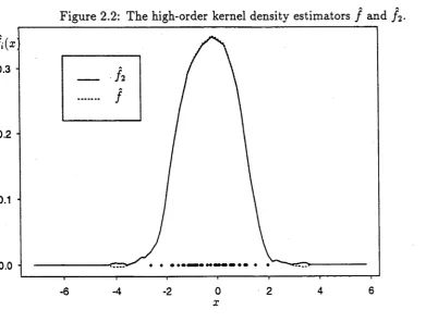
Where it is known that the negative regions of a higher order kernel density estimator occur only in the extreme tails, such as with many unimodal densities, another nonnegative estimator can be constructed. This estimator is obtained by truncating the estimator / outside the “central” range where it is nonnegative, and then renormalising. To do this, define Y\ as the largest value in the lower tail and Y2

as the smallest value in the upper tail, such that f(x) = 0, and to take

h (*) = ~izf(x)I{Yi < x <

r2),

J

Figure 2.2: The high-order kernel density estimators / and f 2.

x

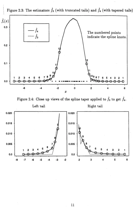
support by tapering the tails within the ranges {c2Y\,CiYi] and [ciY2.c2Y2] where Ci,C2 are fixed constants satisfying 0 < C\ < 1 < c2 < oc. The estimates between C\Y\ and CiY2 are initially the same as for / but are later modified by renormalising. Appropriate values for these constants would be c2 = 2 and Ci = 0.5. Monotone splines based on twelve knots are used to smooth the tails down to zero at c2Y] . i = 1,2. The procedure for the left tail is to break the interval [c2Yi, Yi] into six equal.non­ overlapping subintervals ([ij,tj+\],j = 1, • • • ,6) and another five similar subintervals for [YijCiYi]. That is,

[ctYu Yi] = Uj=i[*j?*j+i] and [ Y ^ c ^ ] = {j)l=7[tj,tj+i} with 11 = c2Yi , £7 = Yi , 112 = C1Y1 .

The first five knots are the coordinates [{tj,g(tj)} , j = 8, • • • , 12] where g(tj) are the same as f{tj) and are positive since m a x (|^ |,j = 8, • • •, 12) < |Yi|. The next six knots are determined in succession by using half the density estimate of the previous knot, ie. [ jtj, ^g(tj+i)I , j = 2, • • •, 7 and the final knot is (t\, 0). A similiar procedure is used for the right tail. This estimator, g , is renormalised using

7 4 = J g ( x ) d x so that / 4 = 74g. (2.4)

Figure 2.3: The estimators / 3 (with truncated tails) and / 4 (with tapered tails).

The numbered points indicate the spline knots.

8 7 6 5 4 3 2 1

Q O O Q O O *Q ”Q Q 0 0 O O

x

Figure 2.4: Close up views of the spline taper applied to / 3 to get / 4.

0.020

0.015

0.010

0.005

0.0

•8 -7 -6 -5 -4 -3 -2 2 3 4 5 6

Left tail Right tail

0.020

0.015

0.010

0.005

We shall show that if the true density has moderately light tails and is unbounded (eg Normal, Gamma, Student’s t), the estimators f x and f 2 have the same asymp­ totic integrated squared error as / .

If the tails of the true density / decrease like a power of |x |_1, then the condition of finite (1 + e)’th order moment, for some e > 0, is both necessary and sufficient for / to have the same asymptotic integrated squared error as f 3 and / 4 . When the underlying distribution is compactly supported (eg Beta), asymptotic equivalence of / and ( f i , i = 1,2,3) is available in a wide range of circumstances.

The principal conclusion to be drawn from this is that /,■ may use the same band­ width as f unless the tails of the density are inordinately large (eg Cauchy). A simulation study in Section 2.4 confirms these statements.

2.3

M a in R e s u lts

2.3.1

In teg ra ted Squared Error P rop erties of th e M ain Es­

tim a to rs

The principal estimators, based on the positive part of / , are

A = 7 1 / / ( / > o), (2.5)

A = 7 2 I / 1. (2.6)

where the positive random variables 71,72 are chosen to ensure that fi and / 2 both integrate to unity. The integral of the negative parts of / is

7 =

J \ f \I(f <

In this notation,

/ / / ( / >

) = / / - / / / ( / <

)

= 1 — ( —7) = 1-4-7

and y I/I =

J f l ( f

Therefore, 7,• = (1 + for i = 1,2 .

Formulae for the ISE of f\ and / 2 depend principally on properties of the random variable 7 which converges to zero as n —> oc. For densities that have continuous derivatives of at least order r, and assuming that h —> 0, nh —» oc as n —* oc. we have for rth order kernel functions that.

where A\ = f K 2, A2 = (Aj^/r!)2 / {/^r^} (with r assumed to be even).

A3 = f f 2, A4 = 2 ( - l ) ~ r/2+lkr/r! f { / ^ }}2 and i = 1 ,2 .

(Similar formulae may be obtained for odd r, but kernels of odd order are seldom used in practice.) The conditions that we stipulated above are the same as those that led to the approximate formula for MISE, given at (1.5), and are available for a wide range of densities. This result permits a simple and direct comparison of the performance of /, and / from the viewpoint of integrated squared error: the performances are asymptotically equivalent if and only if 72 = op {(nh)~l + h2r}.

To prove that the ISE’s of f\ and f2 can be expressed in terms of the random

variable, 7, via equation (2.8), we expand the formulae for the ISE‘s of j \ and f2

using the definitions (2.1) and (2.2). For the ISE of f\ we have,

—=r

/

(A

= / { 7 1 / / ( / > o) - / } 2

=

/ { M l

-m

l

= (27l - ! ) / ( / - f f l C f > 0) + (7i - l) 2 / / 2I ( f > 0)

+

(

: -

) / ( / - / ) / +

J fnf

<

)

-2 (7 i - ! ) / ( / - / ) / / ( / < 0) . (2.9)

A similiar expression for the ISE of f2 is,

/ ( A

= / { 7 2 I / I - / } 2

= j { 7| / 2 - 272| /

I /

/ 2}

+2(72 - 1

- / ) / +

The integrated squared error properties of / are used to further modify equations (2.9) and (2.10). We assume that K is bounded, compactly supported, symmetric. Holder continuous 1 and of r ’th order; and / and its first r derivatives are bounded, continuous and integrable. Under these conditions, Marron and Härdle [15] show that

I S E( h ) - MI S E( h )

MI S E ( h ) 0 as n

or

/ ( / ~ / ) 2/

J E{f

^

The approximation for MISE, given in Silverman [23,p.39ff] and Prakasa Rao [18,Theorem 2.1.7] and previously stated in equation (1.5), is

J

J

J

To further reduce equations (2.9) and (2.10), we need the following results,

J f

j f2I ( f > 0 ) = I P + ° p {! } > (2.14) / ( / - / ) / / ( / < 0 ) = op {(nh)~l + h2r} , (2.15)

J ( f - E f ) f = op{ ( n / t ) " 1/ 2 } , (2.16)

J

(£/

/)

f ( E f — / ) / . The results (2.13), (2.14), (2.15), (2.16) and (2.17) are proved in Section 2.5.

Substituting them into (2.9) we get,

/ - /):

= ( 2 7 1 - 1 )

/ ( /

{ ! - / ( / <

)}

+2(7i - 1)

[~\A^ r

[ / PHI

-2 (7 i - 1) [«^{(nfc)-1 + A2'}]

= {1 + °p(!)} X

; / - / ) 2 + (71 - l ) 2 / / 2 - (71 - 1 ) ^ V + / / 2/ ( / < 0 )} ■ (2.18)

Equation (2.10) can be reduced to give

/ ^ 2 - ^

= (272 - ! ) / ( / - / ) 2 + (72 - l ) 2 { / / 2 + o„(l)}

+ 2 ( 7 2 - 1 ) ~ l j A 4h r + o(hr) + op{ ( n h ) - 1/2} + 472 / ( / < 0) = {1 + °p(!)} x

: / - / ) 2 + (72 - l ) 2 / / 2 - (72 - 1 )A4V + 472 / ( / < 0)} . (2.19)

During the proof of Theorem 2.3 it is shown th a t

and

£ { j T 7 l / | f ( / < 0 ) } = o { (n A )-1} E r2/ ( / < 0)1 = o(h2r) .

term s in (2.18) and (2.19). We also use (7! - 1) ~ - 7 and (72 - 1) ~ - 2 7 , to give

J (/1 — f ) 2 = (1 + °p(l)} *Ai + h 2rA2 + 'y2A3 + "IA^hr + op(/i2r) | = (nh) M i + h A27 2A3 -1- 'yA^h1' -f- op{ h 2r + (n/i) 1 -f 7 2}

and

/ ( A - / ) 2 = { l + oP( l ) } x

(n/i) M i + /i2M 2 -T (27)2A3 + c^'yA\hr4- 472o{(nA) 1}| = (n fc )-M i + /i2M 2(27 ) M 3 + 21 A , h r + op{ h 2r + (nh) ~l + 7 2} ,

which proves th e result (2.8).

2.3.2

D e n sitie s w ith R egu larly V arying Tails

The aim of this section is to find properties of 7 and then su b stitu te into (2.8) to find the ISE of f i and / 2 . We assume th a t the underlying density / has the following properties :

tails th a t decrease as positive powers of |x |-1 as \x\ —> oc,

th a t / > 0 on (—00, + 00) and th a t / has r continuous derivatives satisfying

/ W( 7 ~ { £ ) ' ClX~°' ; / <r)( - * ) ~ ( - l ) r ( 0 c 2x - a^ as n —► oc.

where c i,c 2 > 0 and a i , a 2 > 1 (so th a t / is integrable). (2.20)

The condition we assume of K is th a t

for constants C i.C 2 > 0. A" vanishes outside ( —C1.C1) and

Sometimes we shall strengthen this by requiring that K be Holder continuous. To in­ vestigate the properties of 7 (defined by (2.7)), we first define random variables Z\(v) associated with the right tail of / and Z2(v) (left tail of / ) that have characteristic functions,

A = exp Cj-v aj

J

= exp {—Cji; a>ß(t)} ,/?(*) = j { \ - eltK{y)}dy . (2.22)

The purpose of the random variables Z\(v) and Z2(v) becomes apparent during the proof of Theorem 2.1 (Section 2.5)<where it is shown 'that random variables-^(n, v) =

nhf(x) eonvorgo to Zi(v) (or Z2(v)^ We then define

A s,j = j E[\Zj ( v) \I {Z J( v ) < 0 } \ d v , i = 1,2,

Jo (2.23)

which we use to calculate 7. Under conditions (2.20) and (2.21), and assuming K takes negative values on a set of positive measure, Asj is absolutely convergent to a positive number. This follows from Zj(v) being the limit of a sequence of random variables which, with probability bounded away from zero, take values bounded below zero. Theorem 2.1 shows that 7 is very small so that the ISE of /,• is like the ISE of / •

Theorem 2.1 Assuming the conditions on f (2.20 ) and K (2.21 ) and that h —>

0, nh —> oc as n —>00, we have • + C O

7 =

J_

j= 1 u = 1

If one tail of the underlying density decreases slower than the other, it will exert the dominant influence on 7 (and hence on /,) with the other tail having negligible effect on 7. If both tails decrease at the same rate, both tails influence 7 equally and we only need to calculate 7 for one tail as the other will be the same. To allow for either balanced tails or one tail dominant, we define

a = m in(ai, »2), ^5 = ^ 5,j if c*i ^ ol2 and a = a ;

and A5 = -^5,1 T ^5,2 if QU = <^2- (2.25)

Then equation (2.24) is equivalent to,

7 = {nh)-x+l' aA b+ {(nA)-1+1/“ } . (2.26)

With the result from Theorem 2.1, we may substitute the right side of (2.26) for 7 into the formulae for ISE of (/,-,i = 1,2) (see (2.8) on page 13) to get

J ( f i - f) 2 = (nh)~l Ai +h.'2rA2 + i

+ihr(n h ) - 1+1' aA i As

+op{ ( n h ) - 1 + + ( } . (2.27)

If his chosen so that (n/i)-1 (a factor of the variance) and h2r(a factor of the squared bias) are of the same order, then

I U i - f

?~

/

if and

> 2

is-also optim^-i-m-the sense of minimising-ISE for 2. if and only if a moment higher th an the mean is finite.

The result from Theorem 2.1 is for densities given by (2.20). These conditions may be generalised by including slowly varying functions L\, L2 such that

/<r>(x) = x - ‘“1+r)£ ,(* ) , /M ( - x ) = x - ( ^ +r>i2(x) (2.28)

as x —> oo and c*i, a 2 > 1 . We need only make slight changes to the proof of Theorem 2.1 to accommodate these conditions and the only modifications from the previous result (2.27) are that terms in (n/i)~2+2/Q and (nh)-1+1/Qr are replaced by (n/i)_2+2/QfT3 |( n /i) 1/a j and (nh)~l+l^a L3 j(n /i)1/°'j respectively, where T3 is an­ other slowly varying function. The results due to the generalisations are elucidated in the proof of the theorem.

The former conclusion continues to hold. That is, the bandwidth which is asymp­ totically optimal for minimising the ISE for / is also asymptotically optimal for minimising the ISE for /,-, i = 1,2, provided a > 2, but not if 0 < a < 1. The marginal case a = 2 can go either way depending on the choice of L\ and L2.

Similiar results are readily obtained in a wide range of other cases by adaption of Theorem 2.1. For example, consider densities with exponentially decreasing tails such that

f [r){x) ~ Cn exp ( - c 12i a i) ;

f (r){ - x ) ~ c2\ exp (—c22^0<2)

In such cases, 7 —► 0 and

I (l- f ? = (n h )-1. ^ + h2r + o„ { (n h )-1 + .

We now examine the third density estimator given by

A = 7 3 /(s )/(* i < x < *2), where 73_1 = f f{x)dx ,

J Y \ < S < * 2

Vi is the largest negative solution of f ( x) = 0 and K2 is the smallest positive solution of f ( x) = 0.

We continue to assume that / has at least r derivatives (conditions (2.20)) and strengthen the conditions on K that were given at (2.21) by including Holder continu­ ity. Theorem 2.2 shows that a = m in (a i,a 2) > 2, which is a necessary and sufficient condition for f \ and / 2 to have the same asymptotic ISE as / , is also sufficient for J*3 to share that formula.

T heorem 2.2 The conditions (2.20), (2.21) and K being Holder continuous are as­ sumed, with a > 2 in (2.20). Also it is assumed that for some 0 < e < n -1+£ < h < n~e. Then

J { h ~ S ) 2 = {1 4- Op(1)} {(n/i)-1Ai + h2rA 2] as n -» 00 .

The density estimate / 3 is obtained by truncating / at a point where / goes negative and so the ISE of / 3 will be similiar to the ISE of / if the truncated part is negligible.

The density estimate / 4 is similiar to / 3 but truncated at 2Y2 and we may conclude that

This section concludes with Theorem 2.3 which gives the results that f f 2I { f < 0) and I < 0) are smaller order than (nh)~l. These integrals arise in the expansion

A

of / ( /; — f y given at equations (2.9) and (2.10).

Theorem 2.3 We assume conditions (2.20) regarding derivatives and the tails of f

and conditions (2.21) for the support , bound, symmetry, order and continuity of K ,

and that h = h(n) —> 0 , nh —> oc as n —> oo. Then,

j f 2I ( f < 0 ) + J/ I / I / ( / < 0) = o„ {(n/i)-1} « n - 00 .

2 .3 .3 C o m p a c t ly S u p p o r te d D e n s it ie s

We describe the properties of 7 and of /,-, i = 1,2, 3, in the case where the true density / is supported on a compact interval. Results analogous to those for unboundedly supported densities are derived to show that /,• and / are asymptotically equivalent. Without loss of generality, we may take the support of / to be (0,1). However, the support of /(x ) is close to (—hC\, 1 -f hC\), and to assess 7 we have to consider the contribution to f ( x) outside of (0,1). We assume that / vanishes outside (0,1), / > 0 and has r continuous derivatives on (0,1), and

/ w (x) ~

{i)T ^

-/<')(1 - * ) ~ ( - 1)' ( i ) ' c * x ‘« (2.30)

as x ]. 0 , where c\, ci > 0 and on, > r .

2.1 for densities satisfying (2.30) rather than (2.20). We define the function

Gj (v) = Cj I (v - u)ajK(u)du, (2.31)

J u < v

and put

= - / G< 0).

If K takes negative values then A$,j is strictly positive. If we assume that K is compactly supported, then the integrand in the definition of A $ j vanishes outside a compact set.

Theorem 2.4 Assume conditions (2.21) for K and conditions (2.30) for f , and that

h = h(n) —► 0 and nh —» oo. Then,

7 haj+lAs,j + op < ^2 ha}+l > as n - * oo.

j = i ,j=i

(2.32)

As in Theorem 2.1, we assume that either one tail of the density provides most of the information about 7 or that both tails operate equally. Substituting

7 = ha+1A s + op {ha+l}

into (2.8), we obtain the analogue of (2.27) for densities with compact support,

J(fi- f ) 2 = (nA )-M ! + h2rA2 + i2h2^ r)A 3A\ + 5 +op {(n/i)-1 + h2r + h2^ } 1,2 . (2.33)

However since a > r,

and we may conclude that the integrated squared errors for /,, i = 1,2. and / are asymptotically equivalent when the underlying density has compact support.

We now state an analogue of Theorem 2.2 which gives the ISE for / 3 when the underlying density has compact support. Without loss of generality, we may assume that the support of / is the interval (0,1). Let Y\ and Yj denote respectively the largest solution less than | and the smallest solution greater than | , of f ( x) = 0. Define / 3 by (2.3). Theorem 2.5 shows that / 3 has the same asymptotic ISE as f .

T h eo rem 2.5 Assume that K has support (—C\, C i),\K\ < C2 , is symmetric of

r ’th order, and is Holder continuous. Also assume that for some 0 < e < | , n _1+£ < h < n~c. Then,

j ( h - f ) 2 = {1 + oP( 1)} { (n h )-i A l + .

Theorem 2.6 is the analogue of Theorem 2.3 for compactly supported densities.

T h eorem 2.6 The conditions for K and f are the same as for theorem 2.5. Also, we assume that h = h(n) —> 0 and nh —>00. Then,

J

) + j

) =

)-'

2.4

S im u la tio n S tu d y

We studied each of the estimators / , / 1? / 2, / 3 in the cases of data from Normal, Cauchy, Student’s £, Gamma and Beta distributions and / 4 for Normal, Cauchy and Student’s t distributions and compared the integrated squared errors of / and /, as n —> oo.

The theory in Section 2.3, and its analogue for the Gamma case, predicts that for all but the Cauchy distribution, each type of nonnegative density estimator /,• should have integrated squared error close to that of the basic estimator / , if the same bandwidth is used for all four estimators, and provided that in the Gamma and Beta densities the shape parameters are chosen so that the densities are sufficiently smooth.

2.4.1

S im ulation D eta ils

We took r — 4 throughout, and used the 4’th order kernel suggested by Gasser et al.

[ii],

K{y) = (15/32)(7y4 - 10y2 + 3) /(|y | < 1) . (2.35)

By ensuring that the shape parameters of Gamma and Beta distributions are greater than or equal to 5 we guarantee that / has r = 4 bounded and continuous derivatives on (—oc.oo), except possibly at the origin (for a Gamma distribution with shape parameter 5) or at 0 or 1 (for a Beta distribution with shape parameter 5). where

Conditions (2.21) and Holder continuity are satisfied by K\ condition (2.20) is satisfied by the Cauchy distribution with a = a x = a 2 = 2, and by Student's t distribution with number of degrees of freedom equal to a — 1; condition (2.30) is satisfied by the Beta distribution with shape parameters (ßi, ßi) = (c*i + l , a 2 + 1); and it is straightforward to prove that for the Normal and Gamma distributions, the obvious analogues of our main results hold:

/ ( / . - f f = {1 + Op(l)} {(n/s)-1 + hs A 2}, i = 1,2,3 ,

I f 2 /( / < 0) + / / I / I / ( / < 0) = op{(nh)-' + .

We considered two empirical methods for bandwidth choice, cross-validation (e.g. Sil­ verman [23,p.48ff] and reference to a standard distribution (e.g. Silverman [23,p.45ff]). The latter technique may be developed by noting that by standard asymptotic theory for kernel estimators (Silverman [23.p.66fF]), the optimal bandwidth is given very nearly by

h = 72^ {

J

J

If the underlying distribution were Normal N(n,cr2) then, for the particular kernel given at (2.35), formula (2.36) would reduce to

h = 2.58( i n 's ,

Now, the interquartile range of the normal distribution equals 1.34 times its standard deviation. This observation motivates an empirical rule.

where a denotes sample standard deviation and q is sample interquartile range. By incorporating q into (2.37) we ensure that the bandwidth rule is practicable for heavy­ tailed distributions like the Cauchy.

The cross-validation technique for choosing h requires finding the minimum of a score function,

Ml (h) = n - 2 £ £ K- {h-\Xi- X,)} + 2 n -1/T 1X(0) , where K m(t) = ( K * K)(t) — 2K(t) with ★ being the convolution operator. The score function was initially calculated over a coarse grid of values of h which were multiples (0.25,0.5,1,1.5,2,2.25,2.5) of h as given by (2.37). Then the grid was refined stepwise by locating the current minimum of M\(h) and adding an extra grid point on either side of it. This continued until the relative change in M\(h) was less than 1%.

The computing of K* {h~l (Xi — A',-)} was done by first evaluating K m(t) for 401 values of t 6 [—2,2] and recording these values in a table. For each X{ and only values of X j within two bandwidths of Xi, we referred to the table (interpolating

between the tabulated values if necessary) to get the value of K* {h~l (Xi — Xj)}. By ordering the data and utilising the symmetry of K m(t), the score function was evaluated efficiently.

2.4.2

R esu lts

integrations were performed on grids of at least 200 points.

As our index of the closeness of the integrated squared error of /, to that of / we took

R, = av |ISE(/,) - IS E (/)|/ {av ISE(/)} (2.38)

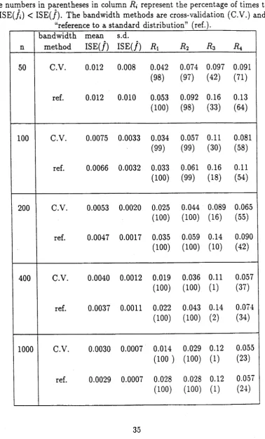
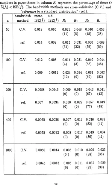
where “av'5 denotes the average over all simulations. We also recorded the number of times that ISE(/t) < ISE(/). These data are summarized in Tables 2.2 to 2.9, for the Normal, Cauchy , Student’s t with 2,4,5,8 degrees of freedom, Gamma (5,1) and Beta (5, 9) distributions respectively, and for the sample sizes n = 50,100,200,400,1000. Relative errors for values of R{. i.e. standard deviations divided by means, are between 7% and 12%.

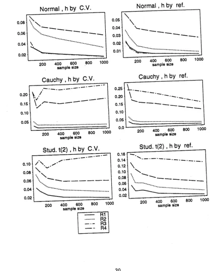
t (2 df) distribution is quite slow and when using cross-validation to estimate h, a sample size of 1000 is insufficient to detect the predicted decrease. This distribution has a (defined at (2.20)) equal to 3. Whilst these tails are lighter than in the critical case of the Cauchy (a = 2), sufficient data can be found in the tails such that 7 does not readily approach zero as n —♦ 0 0.

Data from the Beta distribution are presented because they illustrate the example discussed in Section 2.3.3. As expected, they exhibit similar behaviour to the Normal case, although in the case of Beta data the values of A, converge to zero a little more rapidly. The convergence of A, for the Gamma data is as predicted by the theory.

Figure 2.5: Values of relative difference (i?i) of /, for sample sizes 50,100,200.400,1000 of°Normal (0,1), Cauchy (0,1) and Student’s t (2 df) data.

For graphs on the left, the bandwidth is estimated by cross validation and1 for those on the right, bandwidth is estimated by reference to the Normal distribute .

Norm al, h by ref. Norm al, h by C.V.

400 600

sample size

400 600

sample size

Cauchy , h by C.V. Cauchy , h by ref.

—— . - % _0.25

0.20

0.15

l

I

l

I

I

I

I

0.15

0.10 0.10

0.05 0.05

0.0

N

200 400 600 800

sample size

1000 200 400_{sample size}600 800 1000

400 600

sample size

400 600

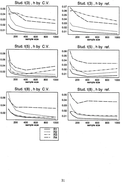
Figure 2.6: Values of relative difference ( Rt) of /, for sample sizes 50,100.200,400,1000 of Student's t (3 df), Student’s t (5 df) and Student’s t (8 df) data.

Stud. t(3) , h by C.V. Stud. t(3) , h by ref.

00 600 sample size

Stud. t ( 5 ) , h by C.V.

00 600 sample size

Stud. t ( 8 ) , h by C.V.

sample size

--- R1 ... R2 --- R3 --- R4

00 600 sample size

Stud. t(5) , h by ref.

00 600 sample size

Stud. t(8) , h by ref.

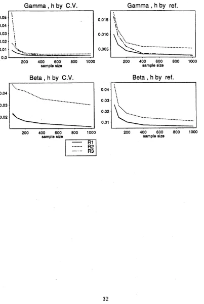
Figure 2.7: Values of relative difference ( Rx) of /, for sample sizes 50.100,200.400,1000 of Gamma(5,l) and Beta(5,9) data.

Gamma , h by C.V. Gamma , h by ref.

0.015

0.010

0.005

00 600

sample size

00 600

sample size

Beta , h by C.V.

sample size

--- R1 ... R2 --- R3

Beta , h by ref.

00 600

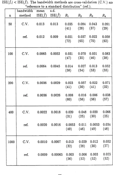
Table 2.2: Values of relative difference (R{) of /,• for sim ulated Normal data. The num bers in parentheses in column R x represent the percentage of times th at

ISE(/{) < IS E (/). The bandw idth m ethods are cross-validation (C.V.) and “reference to a standard distribution” (ref.).

n

bandw idth m ethod

m ean IS E (/)

s.d.

IS E (/)

_Ri

_Rz

50 C.V. 0.013 0.013 0.035

(41) 0.084 (28) 0.043 (37) 0.091 (29)

ref. 0.012 0.009 0.021

(72) 0.037 (65) 0.022 (70) 0.058 (62)

100 C.V. 0.0065 0.0052 0.031

(47) 0.070 (35) 0.031 (46) 0.083 (38)

ref. 0.0064 0.0045 0.014

(58) 0.027 (54) 0.013 (53) 0.052 (55)

200 C.V. 0.0036 0.0029 0.023

(41) 0.057 (30) 0.022 (41) 0.071 (32)

ref. 0.0036 0.0026 0.008

(60) 0.016 (56) 0.006 (56) 0.038 (57)

400 C.V. 0.0022 0.0018 0.020

(31) 0.048 (25) 0.020 (30) 0.066 (25)

ref. 0.0020 0.0016 0.0053

(49) 0.011 (46) 0.0053 (49) 0.034 (48)

1000 C.V. 0.0010 0.0007 0.013

(32) 0.029 (28) 0.012 (30) 0.052 (27)

ref. 0.0009 0.00065 0.003

Table 2.3: Values of relative difference (/?,) of /, for sim ulated Cauchy data. The num bers in parentheses in column Rt represent the percentage of times th at

IS E (/t) < IS E (/). The bandw idth m ethods are cross-validation (C.V.) and “reference to a stan d ard distribution" (ref.).

n

bandw idth m ethod

m ean IS E (/)

s.d.

IS E (/) _{Ri R2 Rz}

50 C.V. 0.015 0.008 0.030

(54) 0.055 (50) 0.21 (57) 0.25 (67)

ref. 0.013 0.010 0.037

(63) 0.068 (58) 0.24 (46) 0.28 (62)

100 C.V. 0.0088 0.0046 0.018

(60) 0.033 (53) 0.17 (38) 0.16 (53)

ref. 0.0072 0.0036 0.023

(62) 0.044 (56) 0.24 (34) 0.21 (51)

200 C.V. 0.0046 0.0023 0.018

(54) 0.033 (51) 0.23 (32) 0.16 (42)

ref. 0.0039 0.0018 0.022

(54) 0.037 (52) 0.23 (28) 0.16 (43)

400 C.V. 0.0027 0.0014 0.016

(50) 0.031 (49) 0.22 (27) 0.15 (38)

ref. 0.0026 0.0013 0.016

(49) 0.033 (46) 0.21 (34) 0.15 (43)

1000 C.V. 0.0012 0.0067 0.013

(45) 0.025 (42) 0.24 (23) 0.17 (31)

ref. 0.0014 0.0006 0.011

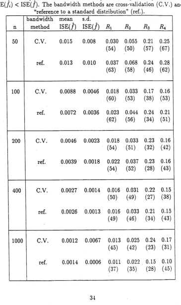
Table 2.4: Values of relative difference (Rt) of /, for sim ulated S tu d en ts't (2 df.) data. The num bers in parentheses in column R t represent the percentage of times th a t

IS E (/,) < IS E (/). The bandw idth m ethods are cross-validation (C.V.) and “reference to a standard d istribution'1 (ref.).

n

bandw idth m ethod

mean IS E (/)

s.d.

IS E (/) Ri R2 Rz

50 C.V. 0.012 0.008 0.042

(98) 0.074 (97) 0.097 (42) 0.091 (71)

ref. 0.012 0.010 0.053

(100) 0.092 (98) 0.16 (33) 0.13 (64)

100 C.V. 0.0075 0.0033 0.034

(99) 0.057 (99) 0.11 (30) 0.081 (58)

ref. 0.0066 0.0032 0.033

(100) 0.061 (99) 0.16 (18) 0.11 (54)

200 C.V. 0.0053 0.0020 0.025

(100) 0.044 (100) 0.089 (16) 0.065 (55)

ref. 0.0047 0.0017 0.035

(100) 0.059 (100) 0.14 (10) 0.090 (42)

400 C.V. 0.0040 0.0012 0.019

(100) 0.036 (100) 0.11 (1) 0.057 (37)

ref. 0.0037 0.0011 0.022

(100) 0.043 (100) 0.14 (2) 0.074 (34)

1000 C.V. 0.0030 0.0007 0.014

(1 0 0 )

0.029 (100) 0.12 (1) 0.055 (23)

ref. 0.0029 0.0007 0.028

Table 2.5: Values of relative difference (/?,) of /,• for sim ulated S tu d en ts't (3 df.) data. The numbers in parentheses in column Rx represent the percentage of times th a t

IS E (/,) < IS E (/). The bandw idth m ethods are cross-validation (C.V.) and “reference to a standard distribution” (ref.).

n

bandw idth m ethod

mean IS E (/)

s.d.

IS E (/) _{Ri R2} Rz R4

50 C.V. 0.018 0.010 0.021

(11) 0.048 (8) 0.040 (45) 0.053 (38)

ref. 0.014 0.008 0.015

(31) 0.031 (22) 0.060 (59) 0.068 (59)

100 C.V. 0.012 0.008 0.014

(4) 0.031 (3) 0.040 (58) 0.044 (45)

ref. 0.009 0.0011 0.024

(12) 0.024 (9) 0.061 (69) 0.062 (53)

200 C.V. 0.0088 0.0046 0.009

(0) 0.019 (0) 0.043 (67) 0.041 (43)

ref. 0.007 0.0034 0.010

(0) 0.022 (0) 0.057 (77) 0.049 (48)

400 C.V. 0.0065 0.0028 0.007

(0) 0.014 (0) 0.036 (82) 0.028 (41)

ref. 0.0055 0.0022 0.008

(0) 0.017 (0) 0.049 (86) 0.034 (41)

1000 C.V. 0.0050 0.0014 0.005

( 0 )

0.010 (0) 0.029 (88) 0.023 (36)

ref. 0.0045 0.0013 0.005

Table 2.6: Values of relative difference (R i) of /, for simulated S tu d en ts't (5 df.) data. The num bers in parentheses in colum n R t represent the percentage of times th at

IS E (/,) < IS E (/). The bandw idth m ethods are cross-validation (C.V.) and “reference to a stan d ard distribution'’ (ref.).

n

bandw idth m ethod

mean IS E (/)

s.d.

IS E (/)

_Ri

_R3

R

50 C.V. 0.016 0.019 0.028

(31) 0.057 (25) 0.090 (38) 0.083 (36)

ref. 0.011 0.009 0.020

(51) 0.038 (44) 0.035 (54) 0.059 (55)

100 C.V. 0.008 0.005 0.016

(24) 0.034 (21) 0.021 (34) 0.048 (31)

ref. 0.007 0.004 0.011

(43) 0.020 (35) 0.027 (46) 0.043 (44)

200 C.V. 0.005 0.003 0.009

(23) 0.019 (19) 0.014 (46) 0.033 (26)

ref. 0.0042 0.0026 0.008

(21) 0.018 (20) 0.016 (43) 0.037 (37)

400 C.V. 0.0032 0.0020 0.006

(16) 0.011 (8) 0.011 (55) 0.025 (16)

ref. 0.0027 0.0014 0.005

(25) 0.009 (12) 0.016 (72) 0.034 (26)

1000 C.V. 0.0019 0.0009 0.004

(22)

0.007 ( 8 )

0.014 (66)

0.025 (18)

ref. 0.0015 0.0006 0.004

Table 2.7: Values of relative difference ( Rt) of /,■ for sim ulated S tu d e n ts't (8 df.) data. The num bers in parentheses in column R x represent the percentage of tim es th a t

IS E (/i) < IS E (/). The bandw idth m ethods are cross-validation (C.V.) and “reference to a stan d a rd distribution'7 (ref.).

n

bandw idth m ethod

mean IS E (/)

s.d.

IS E ( /) _{R i} R2 Rz i?4

50 C.V. 0.012 0.008 0.030

(25) 0.072 (22) 0.031 (31) 0.058 (29)

ref. 0.011 0.008 0.017

(57) 0.033 (53) 0.018 (55) 0.052 (55)

100 C.V. 0.008 0.005 0.021

(21) 0.048 (19) 0.021 (30) 0.047 (29)

ref. 0.006 0.004 0.011

(40) 0.023 (36) 0.019 (45) 0.043 (37)

200 C.V. 0.0040 0.0030 0.012

(14) 0.027 (13) 0.015 (38) 0.035 (20)

ref. 0.0035 0.0026 0.006

(24) 0.013 (21) 0.015 (45) 0.034 (35)

400 C.V. 0.0025 0.0016 0.009

(?) 0.019 (?) 0.010 (28) 0.035 (11)

ref. 0.0020 0.0009 0.005

(9) 0.011 (8) 0.011 (36) 0.038 (19)

1000 C.V. 0.0014 0.0007 0.005

(0) 0.010 (0) 0.010 (36) 0.032 (?)

ref. 0.0012 0.0006 0.004

Table 2.8: Values of relative difference ( R {) of /, for sim ulated G am m a data. The num bers in parentheses in colum n R t represent the percentage of tim es th a t

IS E (/i) < IS E (/). The bandw idth m ethods are cross-validation (C.V.) and “reference to a stan d ard distribution” (ref.).

n

bandw idth m ethod

m ean IS E (/)

s.d.

IS E (/) Ri R2 R3

50 C.V. 0.007 0.005 0.009

(39)

0.018 (30)

0.056 (70)

ref. 0.005 0.003 0.010

(71)

0.017 (64)

0.016 (71)

100 C.V. 0.004 0.003 0.006

(36)

0.011 (30)

0.011 (62)

ref. 0.003 0.002 0.006

(58)

0.011 (51)

0.010 (56)

200 C.V. 0.002 0.001 0.003

(33)

0.006 (32)

0.004 (43)

ref. 0.002 0.0009 0.004

(61)

0.007 (54)

0.006 (62)

400 C.V. 0.001 0.0009 0.002

(33)

0.004 (30)

0.003 (33)

ref. 0.0009 0.0006 0.003

(53)

0.006 (44)

0.003 (48)

1000 C.V. 0.0005 0.0003 0.002

(42)

0.004 (27)

0.002 (43)

ref. 0.0005 0.0003 0.003

(46)

0.005 (37)

Table 2.9: Values of relative difference (Rt) of /, for sim ulated Beta data. The num bers in parentheses in column represent the percentage of times th a t

IS E (/,) < IS E (/). The bandw idth m ethods are cross-validation (C.V.) and “reference to a stan d ard distribution'’ (ref.).

n

bandw idth m ethod

m ean IS E (/)

s.d.

IS E (/) R i R i R z

50 C.V. 0.083 0.062 0.023

(44)

0.047 (34)

0.022 (48)

ref. 0.090 0.076 0.026

(76)

0.045 (71)

0.026 (76)

100 C.V. 0.044 0.033 0.019

(40)

0.043 (23)

0.019 (41)

ref. 0.043 0.029 0.014

(75)

0.025 (66)

0.014 (76)

200 C.V. 0.026 0.021 0.016

(33)

0.042 (26)

0.017 (35)

ref. 0.022 0.013 0.010

(68)

0.018 (57)

0.010 (64)

400 C.V. 0.014 0.011 0.015

(32)

0.035 (20)

0.015 (33)

ref. 0.013 0.009 0.007

(61)

0.014 (48)

0.007 (65)

1000 C.V. 0.007 0.005 0.012

(29)

0.029 (19)

0.012 (29)

ref. 0.006 0.004 0.006

(59)

0.011 (50)

2.5

P r o o fs o f R e s u lts a n d T h e o r e m s

In this section we shall make frequent use of B e rn s te in ’s in eq u a lity (Serfling [22,p.95ff]) and we restate it here because of its importance.

Let Y\ •• - Yn be independent random variables satisfying Pr {|Ti — E(Y{)\ < m} = l, each i, where m < oo. Then for t > 0, and for all n = 1,2 • • • ,

Pr

E ^ - E

_E(y>)

2 x 2

> n i l < 2 exp I ---—---

=---_ / “ I 2 Var(yi) + |mn< (2.39)

2.5.1

P r o o f o f / / 2 = / / 2 + op( 1)

This is statement (2.13) on page 15.

By the triangle inequality, with || • || denoting the L2 metric for functions,

I l l / l l — l l / l l

1 1 /

f \ \ ~

l l / l l

f

<

j E(

which implies that ||/|| —> ||/|| in probability, or equivalently that / f 2 —>• f f 2 in probability.

2.5.2

P r o o f o f f f 2I ( f

>

) =

0

If2

+

o„(l)

This is statement (2.14) on page 15.

We use a result from Theorem 2.3 which is proved later. In that theorem, it is shown that / f 2I ( f < 0) = op { { n h ) ~ 1}. We write the left side of (2.14) as

We now investigate the factor P r ( f < 0). We have that

sup P r ( f < 0) < sup { P r ( |/ - E f \ > |P / |) }

and we can manipulate the RHS of this inequality using Bernstein’s inequality. To identify with the terms in our definition (2.39) on page 41, we write

Yi(:r) = (nh )- l K { h ~ \ x - X;)}

so that f ( x) = Yli=i Yi(x ) and E{ f ( x ) } = E {X)?=i K(^)}- Because the Xi s are inde­ pendent and identically distributed, so to are the s and E{ f ( x ) } = E{Yt(a;)}. Under the i.i.d assumptions, we have that E( f ) = nE(Y\) which is identifiable with the term nt in (2.39) but we retain E ( f ) in the role of nt for convenient evaluation of Bernstein’s inequality. In this notation,

sup [ Pr ( | / - E f \ > |£ / |) } = sup Pr

E 15 - E

_EVi)

We require a bound for |Y{ — E(Yi)\, designated m in (2.39). Since \K\ < C2,

W - E i Y M < \Yi\ + |£{5/,}| < 2( n h ) -

1C2-Thus by Bernstein’s inequality,

_______________

1

and by applying Theorem 2.3 and (2.13) we get (2.14).

2.5.3

P ro o f o f / ( / - f ) f l ( f < 0) = op {(nh) 1 +

}

This is statement (2.15) on page 15.

Let c > 0 be any constant, and write J = {x : f ( x) > c}. We consider the integration

in the left side of (2.15) for the ranges of x given by J and its complement, J . By

Holder’s inequality, 2

e

\J

j

(I - nmf < o)\

<jf

E

\(f

-/ ) / / ( / < o )

< f f } \ i n f P r ( f < $ ) ' ! ' .

We assume (3cc-{2.21)) frhtttr for lcornol function K-r \K\ < -<?2-fft'~€Qaotant)"SO that

■\j---- E f \ < ■{nh)~l GT- Using Bcrnetcm’s inequality'(see (2.39) on--page-44-)-we have

■-t-ha4,

-v*

' sup Pr-( f < 0) sup ----E f \ > \£ / | ) }

. ( \ E f ? 1

n

J r { 2 v a r / + | ( n / !) - 1C 2|£ : / |J

r

Expressions for the expectation and variance of the kernel estimator are given by

E f = f + { K / r \ ) f ^ h r + o(hr) and

var/ = (n /i)-1 /

j

(see Silverman [23, p39]). Thus,

sup P r ( f < 0) = o j(n /i)-1 + h2rJ

and with result (2.12) for the integrated mean square error, we have that

j { f

Since E\(f- / ) / / ( / < 0)| < - f f then,

f . V - n m !

For any e > 0 the right-hand side may be made less than e{(n/i)-1 + h2r}, for all sufficiently large n, by choosing c sufficiently small. The bounds for the integral over the ranges J and J give us the result (2.15).

2 .5 .4 P r o o f o f / ( / — £ ’/ ) / =

op{(n

This is statement (2.16) on page 15.

We first expand the left-hand side as a series of independent variables. That is.

/ ( / - E f ) f = / W 1 j t , K { ( x - X i ) / h } - M f ( M =

L t = i

= n_1 E [A_1 / K {(* - Xi ) / h] f {x)dx - J MS i L

= n - 1 E { / X( y ) f ( Xi - hy)dy -

j

By squaring both sides and taking expectations we have,

e

U O - E f ) f

E {/

J

=

E

E

(/

K(y)f(x

-

hy)dy

-

j Mf

(since the X t are independent ) 21