Computing Convex Coverage Sets
for Faster Multi-objective Coordination
Diederik M. Roijers [email protected]
Shimon Whiteson [email protected]
Frans A. Oliehoek [email protected]
Informatics Institute University of Amsterdam Amsterdam, The Netherlands
Abstract
In this article, we propose new algorithms formulti-objective coordination graphs (MO-CoGs). Key to the efficiency of these algorithms is that they compute a convex coverage set (CCS) instead of a Pareto coverage set (PCS). Not only is a CCS a sufficient solution set for a large class of problems, it also has important characteristics that facilitate more efficient solutions. We propose two main algorithms for computing a CCS in MO-CoGs. Convex multi-objective variable elimination (CMOVE) computes a CCS by performing a series of agent eliminations, which can be seen as solving a series of local multi-objective subproblems. Variable elimination linear support (VELS) iteratively identifies the single weight vector w that can lead to the maximal possible improvement on a partial CCS and calls variable elimination to solve a scalarized instance of the problem forw. VELS is faster than CMOVE for small and medium numbers of objectives and can compute an ε-approximate CCS in a fraction of the runtime. In addition, we propose variants of these methods that employ AND/OR tree search instead of variable elimination to achieve memory efficiency. We analyze the runtime and space complexities of these methods, prove their correctness, and compare them empirically against a naive baseline and an existing PCS method, both in terms of memory-usage and runtime. Our results show that, by focusing on the CCS, these methods achieve much better scalability in the number of agents than the current state of the art.
1. Introduction
In many real-world problem domains, such as maintenance planning (Scharpff, Spaan, Volker, & De Weerdt, 2013) and traffic light control (Pham et al., 2013), multiple agents need to coordinate their actions in order to maximize a common utility. Key to coordinating efficiently in these domains is exploiting loose couplings between agents (Guestrin, Koller, & Parr, 2002; Kok & Vlassis, 2004): each agent’s actions directly affect only a subset of the other agents.
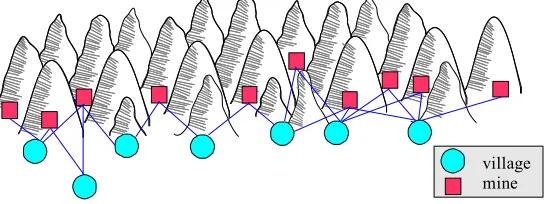
Figure 1: Mining company example.
However, the presence of multiple objectives does not per se necessitate the use of specialized multi-objective solution methods. If the problem can be scalarized, i.e., the utility function can be converted to a scalar utility function, the problem may be solvable with existing single-objective methods. Such a conversion involves two steps (Roijers et al., 2013a). The first step is to specify ascalarization function.
Definition 1. A scalarization functionf, is a function that maps a multi-objective utility of a solution a of a decision problem, u(a), to a scalar utility uw(a):
uw(a) =f(u(a),w),
where w is a weight vector that parameterizes f.
The second step is to define a single-objective version of the decision problem such that the utility of each solutiona equals the scalarized utility of the original problemuw(a).
Unfortunately, scalarizing the problem before solving it is not always possible because w may not be known in advance. For example, consider a company that mines different resources. In Figure 1, we depict the problem this company faces: in the morning one van per village needs to transport workers from that village to a nearby mine, where various resources will be mined. Different mines yield different quantities of resource per worker. The market prices per resource vary through a stochastic process and every price change can alter the optimal assignment of vans. The expected price variation increases with the passage of time. To maximize performance, it is thus critical to act based on the latest possible price information. Since computing the optimal van assignment takes time, redoing this computation for every price change is highly undesirable.
In this article, we consider how multi-objective methods can be made efficient for prob-lems that require the coordination of multiple, loosely coupled agents. In particular, we ad-dressmulti-objective coordination graphs (MO-CoGs): one-shot multi-agent decision prob-lems in which loose couplings are expressed using a graphical model. MO-CoGs form an important class of decision problems. Not only can they be used to model a variety of real-world problems (Delle Fave, Stranders, Rogers, & Jennings, 2011; Marinescu, 2011; Roll´on, 2008), but many sequential decision problems can be modeled as a series of MO-CoGs, as is common in single-objective problems (Guestrin et al., 2002; Kok & Vlassis, 2004; Oliehoek, Spaan, Dibangoye, & Amato, 2010).
Key to the efficiency of the MO-CoG methods we propose is that they compute aconvex coverage set (CCS) instead of a Pareto coverage set (PCS). The CCS is a subset of the PCS that is a sufficient solution for any multi-objective problem with a linear scalarization function. For example, in the mining company example of Figure 1, f is linear, since the total revenue is simply the sum of the quantity of each resource mined times its price per unit. However, even if f is nonlinear, if stochastic solutions are allowed, then a CCS is again sufficient.1
The CCS has not previously been considered as a solution concept for MO-CoGs because computing a CCS requires running linear programs, whilst computing a PCS requires only pairwise comparisons of solutions. However, a key insight of this article2 is that, in loosely coupled systems, CCSs are easier to compute than PCSs, for two reasons. First, the CCS is a (typically much smaller) subset of the PCS. In loosely coupled settings, efficient methods work by solving a series of local subproblems; focusing on the CCS can greatly reduce the size of these subproblems. Second, focusing on the CCS makes solving a MO-CoG equivalent to finding an optimalpiecewise-linear and convex (PWLC)scalarized value function, for which efficient techniques can be adapted. For these reasons, we argue that the CCS is often the concept of choice for MO-CoGs.
We propose two approaches that exploit these insights to solve MO-CoGs more efficiently than existing methods (Delle Fave et al., 2011; Dubus, Gonzales, & Perny, 2009; Marinescu, Razak, & Wilson, 2012; Roll´on & Larrosa, 2006). The first approach deals with the multiple objectives on the level of individual agents, while the second deals with them on a global level.
The first approach extends an algorithm by Roll´on and Larrosa (2006) which we refer to as Pareto multi-objective variable elimination (PMOVE)3, that computes local Pareto sets at each agent elimination, to compute a CCS instead. We call the resulting algorithm
convex multi-objective variable elimination (CMOVE).
The second approach is a new abstract algorithm that we call optimistic linear support (OLS) and is much faster for small and medium numbers of objectives. Furthermore, OLS
1. To be precise, in the case of stochastic strategies a CCS of deterministic strategies is always sufficient (Vamplew, Dazeley, Barker, & Kelarev, 2009); in the case of deterministic strategies, linearity of the scalarization function makes the CCS sufficient (Roijers et al., 2013a).
2. This article synthesizes and extends research already reported in two conference papers. Specifically, the CMOVE algorithm (Section 4) was previously published at ADT (Roijers, Whiteson, & Oliehoek, 2013b) and the VELS algorithm (Section 5) at AAMAS (Roijers, Whiteson, & Oliehoek, 2014). The memory-efficient methods for computing CCSs (Section 6) are a novel contribution of this article. 3. In the original article, this algorithm is calledmulti-objective bucket elimination (MOBE). However, we
can be used to produce a bounded approximation of the CCS, an ε-CCS, if there is not enough time to compute a full CCS. OLS is a generic method that employs single-objective solvers as a subroutine. In this article, we consider two implementations of this subroutine. Usingvariable elimination (VE) as a subroutine yields variable elimination linear support (VELS), which is particularly fast for small and moderate numbers of objectives and is more memory-efficient than CMOVE. However, when memory is highly limited, this reduction in memory usage may not be enough. In such cases, using AND/OR search (Mateescu & Dechter, 2005) instead of VE yields AND/OR tree search linear support (TSLS), which is slower than VELS but much more memory efficient.
We prove the correctness of both CMOVE and OLS. We analyze the runtime and space complexities of both methods and show that our methods have better guarantees than PCS methods. We show CMOVE and OLS are complementary, i.e., various trade-offs exist between them and their variants.
Furthermore, we demonstrate empirically, on both randomized and more realistic prob-lems, that CMOVE and VELS scale much better than previous algorithms. We also empir-ically confirm the trade-offs between CMOVE and OLS. We show that OLS, when used as a bounded approximation algorithm, can save additional orders of magnitude of runtime, even for small ε. Finally, we show that, even when memory is highly limited, TSLS can still solve large problems.
The rest of this article is structured as follows. First, we provide a formal definition of our model, as well as an overview of existing solution methods in Section 2. After presenting a naive approach in Section 3, in Sections 4, 5 and 6, we analyze the runtime and space complexities of each algorithm, and compare them empirically, against each other and existing algorithms, at the end of each section. Finally, we conclude in Section 7 with an overview of our contributions and findings, and suggestions for future research.
2. Background
In this section, we formalize themulti-objective coordination graph (MO-CoG). Before doing so however, we describe the single-objective version of this problem, thecoordination graph
(CoG), of which the MO-CoG is an extension, and thevariable elimination (VE) algorithm for solving CoGs. The methods we present in Section 4 and 5 build on VE in different ways.
2.1 (Single-Objective) Coordination Graphs
Acoordination graph(CoG) (Guestrin et al., 2002; Kok & Vlassis, 2004) is a tuplehD,A,U i, where
• D={1, ..., n} is the set of nagents,
• A=Ai×...× An is the joint action space: the Cartesian product of the finite action
spaces of all agents. A joint action is thus a tuple containing an action for each agent a=ha1, ..., ani, and
• U=
u1, ..., uρ is the set ofρ scalarlocal payoff functions, each of which has limited
scope, i.e., it depends on only a subset of the agents. The total team payoff is the sum of the local payoffs: u(a) =Pρ
Figure 2: (a) A CoG with 3 agents and 2 local payoff functions (b) after eliminating agent 3 by addingu3 (c) after eliminating agent 2 by addingu4.
˙
a2 ¯a2 ˙
a1 3.25 0 ¯
a1 1.25 3.75
˙ a3 ¯a3 ˙
a2 2.5 1.5 ¯
[image:5.612.211.403.269.318.2]a2 0 1
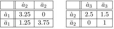
Table 1: The payoff matrices for u1(a1, a2) (left) and u2(a2, a3) (right). There are two possible
actions per agent, denoted by a dot ( ˙a1) and a bar (¯a1).
All agents share the payoff functionu(a). We abuse the notationeto both index a local payoff function ue and to denote the subset of agents in its scope; ae is thus a local joint
action, i.e., a joint action of this subset of agents.
The decomposition of u(a) into local payoff functions can be represented as a factor graph (Bishop, 2006), a bipartite graph containing two types of vertices: agents (variables) and local payoff functions (factors), with edges connecting local payoff functions to the agents in their scope.
Figure 2a shows the factor graph of an example CoG in which the team payoff function decomposes into two local payoff functions, each with two agents in scope:
u(a) =
ρ
X
e=1
ue(ae) =u1(a1, a2) +u2(a2, a3).
The local payoff functions are defined in Table 1. The factor graph illustrates the loose couplings that result from the decomposition into local payoff functions. In particular, each agent’s choice of action directly depends only on those of its immediate neighbors, e.g., once agent 1 knows agent 2’s action, it can choose its own action without considering agent 3.
2.2 Variable Elimination
We now discuss the variable elimination (VE) algorithm, on which several multi-objective extensions (Roll´on & Larrosa, 2006; Roll´on, 2008) build, including our own CMOVE algo-rithm (Section 4). We also use VE as a subroutine in the OLS algoalgo-rithm (Section 5).
pass, VE eliminates each of the agents in turn by computing the value of that agent’s best response to every possible joint action of its neighbors. These values are used to construct a new local payoff function that encodes the value of the best response and replaces the agent and the payoff functions in which it participated. In the original algorithm, once all agents are eliminated, a backward pass assembles the optimal joint action using the constructed payoff functions. Here, we present a slight variant in which each payoff is ‘tagged’ with the action that generates it, obviating the need for a backwards pass. While the two algorithms are equivalent, this variant is more amenable to the multi-objective extension we present in Section 4.
VE eliminates agents from the graph in a predetermined order. Algorithm 1 shows pseudocode for the elimination of a single agent i. First, VE determines the set of local payoff functions connected toi,Ui, and the neighboring agents ofi,ni (lines 1-2).
Definition 2. The set of neighboring local payoff functions Ui of i is the set of all local payoff functions that have agent i in scope.
Definition 3. The set of neighboring agents of i, ni, is the set of all agents that are in
scope of one or more of the local payoff functions in Ui.
Then, it constructs a new payoff function by computing the value of agent i’s best response to each possible joint action ani of the agents in ni (lines 3-12). To do so, it
loops over all these joint actions Ani (line 4). For each ani, it loops over all the actionsAi
available to agent i (line 6). For each ai ∈ Ai, it computes the local payoff when agent i
responds toani withai (line 7). VE tags the total payoff withai, the action that generates
it (line 8) in order to be able to retrieve the optimal joint action later. If there are already tags present, VE appends ai to them; in this way, the entire joint action is incrementally
constructed. VE maintains the value of the best response by taking the maximum of these payoffs (line 11). Finally, it eliminates the agent and all payoff functions in Ui and replaces them with the newly constructed local payoff function (line 13).
Algorithm 1:elimVE(U, i) Input: A CoGU, and an agenti
1 Ui ←set of local payoff functions involvingi 2 ni ←set of neighboring agents ofi
3 unew ←a new factor taking joint actions ofni,ani, as input 4 foreach ani ∈ Ani do
5 S ← ∅
6 foreachai∈ Ai do
7 v←
X
uj∈Ui
uj(ani, ai)
8 tagv withai 9 S ← S ∪ {v}
10 end
11 unew(ani)←max(S) 12 end
Consider the example in Figure 2a and Table 1. The optimal payoff maximizes the sum of the two payoff functions:
max
a u(a) = maxa1,a2,a3
u1(a1, a2) +u2(a2, a3).
If VE eliminates agent 3 first, then it pushes the maximization over a3 inward such that goes only over the local payoff functions involving agent 3, in this case just u2:
max
a u(a) = maxa1,a2
u1(a1, a2) + max
a3
u2(a2, a3)
.
VE solves the inner maximization and replaces it with a new local payoff function u3 that depends only on agent 3’s neighbors, thereby eliminating agent 1:
max
a u(a) = maxa1,a2
u1(a1, a2) +u3(a2)
,
which leads to the new factor graph depicted in Figure 2b. The values ofu3(a2) areu3( ˙a2) = 2.5, using ˙a3, and u3(¯a2) = 1 using ¯a3, as these are the optimal payoffs for the actions of agent 2, given the payoffs shown in Table 1. Because we ultimately want the optimal joint action, not just the optimal payoff, VE tags each payoff of u3 with the action of agent 3 that generates it, i.e., we can think ofu3(a2) as a (value,tag) pair. We denote such a pair with parentheses and a subscript: u3( ˙a2) = (2.5)˙a3, and u
3(¯a2) = (1)¯
a3.
VE next eliminates agent 2, yielding the factor graph shown in Figure 2c:
max
a u(a) = maxa1
max
a2
u1(a1, a2) +u3(a2)
= max
a1
u4(a1).
VE appends the new tags for agent 2 to the existing tags for agent 3, yielding the following tagged payoff values: u4( ˙a1) = maxa2u
1( ˙a
1, a2) +u3(a2) =(3.25)a˙2+ (2.5)˙a2a˙3 = (5.75)˙a2a˙3
andu4(¯a1) = (3.75)¯a2+ (1)¯a2a¯3 = (4.75)¯a2¯a3. Finally, maximizing overa1 yields the optimal
payoff of (5.75)a˙1a˙2a˙3, with the optimal action contained in the tags.
The runtime complexity of VE is exponential, not in the number of agents, but only in theinduced width, which is often much less than the number of agents.
Theorem 1. The computational complexity of VE is O(n|Amax|w) where |A
max| is the
maximal number of actions for a single agentandw is the induced width, i.e., the maximal number of neighboring agents of an agent plus one (the agent itself ), at the moment when it is eliminated (Guestrin et al., 2002).
Theorem 2. The space complexity of VE isO(n|Amax|w).
This space complexity arises because, for every agent elimination, a new local payoff function is created with O(|Amax|w) fields (possible input actions). Since it is impossible
to tell a priori how many of these new local payoff functions exist at any given time during the execution of VE, this need to be multiplied by the total number of new local payoff functions created during a VE execution, which isn.
While VE is designed to minimize runtime4 other methods focus on memory efficiency instead (Mateescu & Dechter, 2005). We discuss memory efficiency further in Section 6.1.
˙
a2 a¯2 ˙
a1 (4,1) (0,0) ¯
a1 (1,2) (3,6)
˙
a3 ¯a3 ˙
a2 (3,1) (1,3) ¯
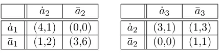
[image:8.612.199.414.87.139.2]a2 (0,0) (1,1) Table 2: The two-dimensional payoff matrices foru1(a
1, a2) (left) andu2(a2, a3) (right).
2.3 Multi-objective Coordination Graphs
A multi-objective coordination graph (MO-CoG) is a tuple hD,A,U i in which Dand Aare as before but, U =
u1, ...,uρ is now a set of ρ,d-dimensionallocal payoff functions. The total team payoff is the sum of local vector-valued payoffs: u(a) = Pρ
e=1ue(ae). We use
ui to indicate the value of the i-th objective. We denote the set of all possible joint action
values as V. Table 2 shows a two-dimensional MO-CoG with the same structure as the single-objective example in Section 2.1, but with multi-objective payoffs.
The solution to a MO-CoG is acoverage set (CS)of joint actionsaand associated values u(a) that contains at least one optimal joint action for each possible parameter vector w of the scalarization function f (Definition 1). A CS is a subset of theundominated set:
Definition 4. The undominated set (U) of a MO-CoG, is the set of all joint actions and associated payoff values that are optimal for some wof the scalarization function f.
U(V) =
u(a) : u(a)∈ V ∧ ∃w∀a0 uw(a)≥uw(a0) .
Because we care about having at least one optimal joint action for everyw, rather than all optimal joint actions, a lossless subset of U suffices:
Definition 5. Acoverage set (CS),CS(V), is a subset of U, such that for each possiblew, there is at least one optimal solution in the CS, i.e.,
∀w∃a u(a)∈CS(V)∧ ∀a0 uw(a)≥uw(a0)
.
Note that the CS is not necessarily unique. Typically we seek the smallest possible CS. For convenience, we assume that payoff vectors in the CS contain both the values and associated joint actions, as suggested by the tagging scheme described in Section 2.2.
Which payoff vectors from V should be in the CS depends on what we know about the scalarization functionf. A minimal assumption is that f is monotonically increasing, i.e., if the value for one objective ui, increases while all uj6=i stay constant, the scalarized value
u(a) cannot decrease. This assumption ensures that objectives are desirable, i.e., all else being equal, having more of them is always better.
Definition 6. The Pareto frontis the undominated set for arbitrary strictly monotonically increasing scalarization functionsf.
P F(V) =u(a) :u(a)∈ V ∧ ¬∃a0 u(a0)P u(a) ,
whereP indicates Pareto dominance (P-dominance): greater or equal in all objectives and
In order to have all optimal scalarized values, it is not necessary to compute the entire PF. E.g., if two joint actions have equal payoffs we need to retain only one of those.
Definition 7. A Pareto coverage set (PCS), P CS(V) ⊆ P F(V), is a coverage set for arbitrary strictly monotonically increasing scalarization functions f, i.e.,
∀a0∃a u(a)∈P CS(V)∧(u(a)Pu(a0)∨u(a) =u(a0))
.
Computing P-dominance requires only pairwise comparison of payoff vectors (Feng & Zilberstein, 2004).5
A highly prevalent scenario is that, in addition to f being monotonically increasing, we also know that it is linear, that is, the parameter vectors w are weights by which the values of the individual objectives are multiplied,f =w·u(a). In the mining example from Figure 1, resources are traded on an open market and all resources have a positive unit price. In this case, the scalarization is a linear combination of the amount of each resource mined, where the weights correspond to the price per unit of each resource. Many more examples of linear scalarization functions exist in the literature, e.g., (Lizotte, Bowling, & Murphy, 2010). Because we assume the linear scalarization is monotonically increasing, we can represent it without loss of generality as a convex combination of the objectives: i.e., the weights are positive and sum to 1. In this case, only a convex coverage set (CCS) is needed, which is a subset of theconvex hull (CH)6:
Definition 8. The convex hull (CH) is the undominated set for linear non-decreasing scalarizations f(u(a),w) =w·u(a):
CH(V) =
u(a) :u(a)∈ V ∧ ∃w∀a0 w·u(a)≥w·u(a0) .
That is, the CH contains all solutions that attain the optimal value for at least one weight. Vectors not in the CH areC-dominated. In contrast to P-domination, C-domination cannot be tested for with pairwise comparisons because it can take two or more payoff vectors to C-dominate a payoff vector. Note that the CH contains more solutions than needed to guar-antee an optimal scalarized value value: it can contain multiple solutions that are optimal for one specific weight. A lossless subset of the CH with respect to linear scalarizations is called a convex coverage set (CCS), i.e., a CCS retains at least one u(a) that maximizes the scalarized payoff, w·u(a), for every w:
Definition 9. A convex coverage set (CCS), CCS(V) ⊆CH(V), is a CS for linear non-decreasing scalarizations, i.e.,
∀w∃a u(a)∈CCS(V)∧ ∀a0 w·u(a)≥w·u(a0).
Since linear non-decreasing functions are a specific type of monotonically increasing func-tion, there is always a CCS that is a subset of the smallest possible PCS.
As previously mentioned, CSs like the PCS and CCS, may not be unique. For example, if there are two joint actions with equal payoff vectors, we need at most one of them to make a PCS or CCS.
5. P-dominance is often calledpairwise dominancein the POMDP literature.
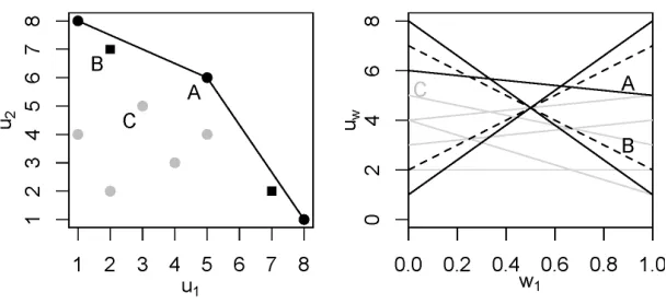
Figure 3: The CCS (filled circles at left, and solid black lines at right) versus the PCS (filled circles and squares at left, and both dashed and solid black lines at right) for twelve random 2-dimensional payoff vectors.
In practice, the PCS and the CCS are often equal to the PF and CH. However, the algorithms proposed in this article are guaranteed to produce a PCS or a CCS, and not necessarily the entire PF or the CH. Because PCSs and the CCSs are sufficient solutions in terms of scalarized value, we say that these algorithms solve the MO-CoGs.
In Figure 3 (left) the values of joint actions, u(a), are represented as points in value-space, for a two-objective MO-CoG. The joint action valueA is in both the CCS and the PCS.B, however, is in the PCS, but not the CCS, because there is no weight for which a linear scalarization ofB’s value would be optimal, as shown in Figure 3 (right), where the scalarized value of the strategies are plotted as a function of the weight on the first objective (w2 = 1−w1). C is in neither the CCS nor the PCS: it is Pareto-dominated by A.
Many multi-objective methods, e.g., (Delle Fave et al., 2011; Dubus et al., 2009; Mari-nescu et al., 2012; Roll´on, 2008) simply assume that the PCS is the appropriate solution concept. However, we argue that the choice of CS depends on what one can assume about how utility is defined with respect to the multiple objectives, i.e., which scalarization func-tion is used to scalarize the vector-valued payoffs. We argue that in many situafunc-tions the scalarization function is linear, and that in such cases one should use the CCS.
In addition to the shape of f, the choice of solution concept depends on whether only deterministic joint actions are considered or whether stochastic strategies are also permit-ted. A stochastic strategy π assigns a probability to each joint action A → [0,1]. The probabilities for all joint actions together sum to 1,P
a∈Aπ(a) = 1. The value of a stochas-tic strategy is a linear combination of the value vectors of the joint actions of which it is a mixture: uπ = P
a∈Aπ(a)u(a). Therefore, the optimal values, for any monotonically increasing f, lie on the convex upper surface spanned by the strategies in the CCS, as indicated by the lines in Figure 3 (left). Therefore, all optimal values for monotonically increasing f, including nonlinear ones, can be constructed by taking mixture policies from the CCS (Vamplew et al., 2009).
smaller. This is particularly important when the final selection of the joint is done by (a group of) humans, who have to compare all possible alternatives in the solution set.
The methods presented in this article are based onvariable elimination (VE) (Sections 4 and 5) and AND/OR tree search (TS) (Section 6). These algorithms are exact solution methods for CoGs.
The CMOVE algorithm we propose in Section 5 is based on VE. It differs from another multi-objective algorithm based on VE, which we refer to as PMOVE (Roll´on & Larrosa, 2006), in that it produces a CCS rather than a PCS. An alternative to VE are message-passing algorithms, like max-plus (Pearl, 1988; Kok & Vlassis, 2006a). However, these are guaranteed to be exact only for tree-structured CoGs. Multi-objective methods that build on max-plus such as that of Delle Fave et al. (2011), have this same limitation, unless they preprocess the CoG to form a clique-tree or GAI network (Dubus et al., 2009). On tree structured graphs, both message-passing algorithms and VE produce optimal solutions with similar runtime guarantees. Note that, like PMOVE, existing multi-objective methods based on message passing produce a PCS rather than a CCS.
In Section 5, we take a different approach to multi-objective coordination based on an
outer loop approach. As we explain, this approach is applicable only for computing a CCS, not a PCS, but has considerable advantages in terms of runtime and memory usage.
3. Non-graphical Approach
A naive way to compute a CCS is to ignore the graphical structure, calculate the set of all possible payoffs for all joint actions V, and prune away the C-dominated joint actions. We first translate the problem to a set ofvalue set factors (VSFs),F. Each VSFf is a function mapping local joint actions to sets of payoff vectors. The initial VSFs are constructed from the local payoff functions such that
fe(ae) ={ue(ae)},
i.e., each VSF maps a local joint action to the singleton set containing only that action’s local payoff. We can now defineV in terms ofF using thecross-sum operator over all VSFs inF for each joint actiona:
V(F) =[ a
M
fe∈F
fe(ae),
where the cross-sum of two setsA andB contains all possible vectors that can be made by summing one payoff vector from each set:
A⊕B={a+b:a∈A∧b∈B}.
The CCS can now be calculated by applying a pruning operatorCPrune(described below) that removes all C-dominated vectors from a set of value vectors, toV:
CCS(V(F)) =CPrune(V(F)) =CPrune([ a
M
fe∈F
fe(ae)). (1)
A CCS contains at least one payoff vector that maximizes the scalarized value for every w:
∀w a= arg max a∈A
w·u(a) =⇒ ∃a0 u(a0)∈CCS(V(F)) ∧ w·u(a) =w·u(a0). (2)
That is, for every w there is an solution a0 that is part of the CCS and that achieves the same value as a maximizing solutiona. Moreover the value of such solutions is given by the dot product. Thus, finding the CCS is analogous to the problem faced inpartially observable Markov decision processes (POMDPs) (Feng & Zilberstein, 2004), where optimalα-vectors (corresponding to the value vectorsu(a)) for all beliefs (corresponding to the weight vectors w) must be found. Therefore, we can employ pruning operators from POMDP literature.
Algorithm 2 describes our implementation ofCPrune, which is based on that of Feng and Zilberstein (2004) with one modification. In order to improve runtime guarantees,CPrune first pre-prunes the candidate solutionsU to a PCS using the PPrune(Algorithm 3) at line 1. PPrune computes a PCS in O(d|U ||P CS|) by running pairwise comparisons. Next, a partial CCS, U∗, is constructed as follows: a random vector u from U is selected at line 4. For u the algorithm tries to find a weight vector w for whichu is better than the vectors in U∗(line 5), by solving the linear program in Algorithm 4. If there is such a w,CPrune finds the best vectorvforwinU and moves it toU∗(line 11–13). If there is no weight for which u is better it is C-dominated and thus removedu fromU (line 8).
Algorithm 2:CPrune(U) Input: A set of payoff vectorsU
1 U ←PPrune(U) 2 U∗← ∅
3 while notEmpty(U)do 4 select randomufromU 5 w←findWeight(u,U∗) 6 if w=null then
7 //did not find a weight whereuis optimal 8 removeufrom U
9 end 10 else
11 v←arg maxu∈Uw·u 12 U ← U \ {v}
13 U∗← U∗∪ {v} 14 end
15 end 16 returnU∗
The runtime of CPruneas defined by Algorithm 2 is
O(d|U ||P CS|+|P CS|P(d|CCS|)), (3)
Algorithm 3:PPrune(U) Input: A set of payoff vectorsU
1 U∗← ∅
2 while U 6=∅do
3 u←the first element ofU 4 foreach v∈ U do
5 if vP u then
6 u←v // Continue withv instead ofu
7 end
8 end
9 Removeu, and all vectors P-dominated byu, from U 10 AddutoU∗
11 end 12 returnU∗
Algorithm 4: findWeight(u,U)
max
x,w x
subject to w·(u−u0)−x≥0,∀u0 ∈ U
d
X
i=1
wi = 1
if x>0 return w else returnnull
The key downside of the non-graphical approach is that it requires explicitly enumerating all possible joint actions and calculating the payoffs associated with each one. Consequently, it is intractable for all but small numbers of agents, as the number of joint actions grows exponentially in the number of agents.
Theorem 3. The time complexity of computing a CCS of a MO-CoG containing ρ local payoff functions, following the non-graphical approach (Equation 1) is:
O(dρ|Amax|n+d|A
max|n|P CS|+|P CS|P(d|CCS|)
Proof. First, V is computed by looping over all ρ VSFs for each joint action a, summing vectors of length d. If the maximum size of the action space of an agent is Amax there are
O(|Amax|n) joint actions. V contains one payoff vector for each joint action. V is the input
of CPrune.
In the next two sections, we present two approaches to compute CCSs more efficiently. The first approach pushed the CPrune operator in Equation 1 into the cross-sum and union, just as the max-operator is pushed into the summation in VE. We call this the
1988), a POMDP pruning operator that only requires finding the optimal solution for cer-tain w. Instead of performing maximization over the entire setV, as in the original linear support algorithm, we show that we can use VE on a finite number ofscalarized instances of the MO-CoG, avoiding explicit calculation of V. We call this approach the outer loop approach, as this it creates an outer loop around a single objective method (like VE), which it calls as a subroutine.
4. Convex Variable Elimination for MO-CoGs
In this section we show how to exploit loose couplings and calculate a CCS using an in-ner loop approach, i.e., by pushing the pruning operators into the cross-sum and union operators of Equation 1. The result is CMOVE, an extension to Roll´on and Larrosa’s Pareto-based extension of VE, which we refer to as PMOVE (Roll´on & Larrosa, 2006). By analyzing CMOVE’s complexity in terms of local convex coverage sets, we show that this approach yields much better runtime complexity guarantees than the non-graphical approach to computing CCSs that was presented in Section 3.
4.1 Exploiting Loose Couplings in the Inner Loop
In the non-graphical approach, computing a CCS is more expensive than computing a PCS, as we have shown in Section 3. We now show that, in MO-CoGs, we can compute a CCS much more efficiently by exploiting the MO-CoG’s graphical structure. In particular, like in VE, we can solve the MO-CoG as a series of local subproblems, byeliminating agents and manipulating the set of VSFsF which describe the MO-CoG. The key idea is to compute
local CCSs (LCCSs)when eliminating an agent instead of a single best response (as in VE). When computing an LCCS, the algorithm prunes away as many vectors as possible. This minimizes the number of payoff vectors that are calculated at the global level, which can greatly reduce computation time. Here we describe theelimoperator for eliminating agents used by CMOVE in Section 4.2.
We first need to update our definition of neighboring local payoff functions (Definition 2), to neighboring VSFs.
Definition 10. The set of neighboring VSFsFi of i is the set of all local payoff functions that have agent iin scope.
The neighboring agents ni of an agent i are now the agents in the scope of a VSF in
Fi, except fori itself, corresponding to Definition 3. For each possible local joint action of ni, we now compute an LCCS that contains the payoffs of the C-undominated responses of
agenti, as the best response values ofi. In other words, it is the CCS of the subproblem that arises when considering onlyFi and fixing a specific local joint actionani. To compute the
LCCS, we must consider all payoff vectors of the subproblem,Vi, and prune the dominated
ones.
Definition 11. If we fix all actions in ani, but not ai, the set of all payoff vectors for this subproblem is: Vi(Fi,ani) =
S
ai L
fe∈F if
e(a
e), where ae is formed from ai and the
appropriate part of ani.
Definition 12. A local CCS, an LCCS, is the C-undominated subset of Vi(Fi,ani):
LCCSi(Fi,ani) =CCS(Vi(Fi,ani)).
Using these LCCSs, we can create a new VSF, fnew, conditioned on the actions of the agents in ni:
∀ani f
new(a
ni) =LCCSi(Fi,ani).
The elimoperator replaces the VSFs in Fi inF by this new factor:
elim(F, i) = (F \ Fi)∪ {fnew(ani)}.
Theorem 4. elim preserves the CCS: ∀i ∀F CCS(V(F)) =CCS(V(elim(F, i))).
Proof. We show this by using the implication of Equation 2, i.e., for all joint actions afor which there is a w at which the scalarized value of a is maximal, a vector-valued payoff u(a0) for which w·u(a0) = w·u(a0) is in the CCS. We show that the maximal scalarized payoff cannot be lost as a result ofelim.
The linear scalarization function distributes over the local payoff functions: w·u(a) = w·P
eue(ae) =
P
ew·ue(ae).Thus, when eliminating agent i, we divide the set of VSFs
into non-neighbors (nn), in which agent i does not participate, and neighbors (ni) such
that:
w·u(a) = X
e∈nn
w·ue(ae) +
X
e∈ni
w·ue(ae).
Now, following Equation 2, the CCS contains maxa∈Aw·u(a) for all w. elim pushes this maximization in:
max
a∈Aw·u(a) =a−maxi∈A−i X
e∈nn
w·ue(ae) + max ai∈Ai
X
e∈ni
w·ue(ae).
elim replaces the agent-i factors by a term fnew(ani) that satisfies w·f
new(a
ni) = maxai P
e∈niw·u
e(a
e) per definition, thus preserving the maximum scalarized value for allwand
thereby preserving the CCS.
Instead of an LCCS, we could compute a local PCS (LPCS), that is, using a PCS computation on Vi instead of a CCS computation. Note that, since LCCS ⊆ LPCS ⊆ Vi, elim not only reduces the problem size with respect to Vi, it can do so more than would
4.2 Convex Multi-objective Variable Elimination
We now present theconvex multi-objective variable elimination (CMOVE)algorithm, which implements elim using CPrune. Like VE, CMOVE iteratively eliminates agents until none are left. However, our implementation of elim computes a CCS and outputs the correct joint actions for each payoff vector in this CCS, rather than a single joint action. CMOVE is an extension to Roll´on and Larrosa’s Pareto-based extension of VE, which we refer to as PMOVE (Roll´on & Larrosa, 2006).
The most important difference between CMOVE and PMOVE is that CMOVE com-putes a CCS, which typically leads to much smaller subproblems and thus much better computational efficiency. In addition, we identify three places where pruning can take place, yielding a more flexible algorithm with different trade-offs. Finally, we use the tag-ging scheme instead of thebackwards pass, as in Section 2.2.
Algorithm 5 presents an abstract version of CMOVE that leaves the pruning operators unspecified. As in Section 3, CMOVE first translates the problem into a set of vector-set factors (VSFs),F on line 1. Next, CMOVE iteratively eliminates agents usingelim (line 2–5). The elimination order can be determined using techniques devised for single-objective VE (Koller & Friedman, 2009).
Algorithm 5:CMOVE(U,prune1,prune2,prune3,q)
Input: A set of local payoff functionsU and an elimination orderq(a queue containing all agents)
1 F ← create one VSF for every local payoff function inU 2 while ani∈ Ani do
3 i←q.dequeue()
4 F ←elim(F, i,prune1,prune2) 5 end
6 f ←retrieve final factor from F 7 S ←f(a∅)
8 returnprune3(S)
Algorithm 6 shows our implementation of elim, parameterized with two pruning op-erators, prune1 and prune2, corresponding to two different pruning locations inside the operator that computesLCCSi: ComputeLCCSi(Fi,ani,prune1,prune2).
Algorithm 6:elim(F, i,prune1,prune2) Input: A set of VSFs F, and an agenti
1 ni ←the set of neighboring agents ofi 2 Fi←the subset of VSF that haveiin scope 3 fnew(ani)←a new VSF
4 foreach ani ∈ Ani do
5 fnew(ani)←ComputeLCCSi(Fi,ani,prune1,prune2) 6 end
7 F ← F \ Fi∪ {fnew}
ComputeLCCSi is implemented as follows: first we define a new cross-sum-and-prune
operatorA⊕ˆB =prune1(A⊕B). LCCSi applies this operator sequentially:
ComputeLCCSi(Fi,ani,prune1,prune2) =prune2( [
ai
ˆ M
fe∈F i
fe(ae)). (4)
prune1is applied to each cross-sum of two sets, via the ˆ⊕operator, leading to incremental pruning (Cassandra, Littman, & Zhang, 1997). prune2is applied at a coarser level, after the union. CMOVE applies elim iteratively until no agents remain, resulting in a CCS. Note that, when there are no agents left, fnew on line 3 has no agents to condition on. In this case, we consider the “actions of the neighbors” to be a single empty action: a∅.
Pruning can also be applied at the very end, after all agents have been eliminated, which we callprune3. In increasing level of coarseness, we thus have three pruning opera-tors: incremental pruning (prune1), pruning after the union over actions of the eliminated agent (prune2), and pruning after all agents have been eliminated (prune3), as reflected in Algorithm 5. After all agents have been eliminated, the final factor is taken from the set of factors (line 6), and the single set,S contained in that factor is retrieved (line 7). Note that we use the empty action a∅ to denote the field in the final factor, as it has no agents in scope. Finallyprune3is called on S.
Consider the example in Figure 2a, using the payoffs defined by Table 2, and apply CMOVE. First, CMOVE creates the VSFsf1andf2 fromu1 andu2. To eliminate agent 3, it creates a new VSFf3(a2) by computing the LCCSs for everya2and tagging each element of each set with the action of agent 3 that generates it. For ˙a2, CMOVE first generates the set {(3,1)˙a3,(1,3)¯a3}. Since both of these vectors are optimal for some w, neither is
removed by pruning and thusf3( ˙a2) ={(3,1)a˙3,(1,3)¯a3}. For ¯a2, CMOVE first generates {(0,0)a˙3,(1,1)a¯3}. CPrunedetermines that (0,0)a˙3 is dominated and consequently removes
it, yielding f3(¯a2) = {(1,1)¯a3}. CMOVE then adds f
3 to the graph and removes f2 and agent 3, yielding the factor graph shown in Figure 2b.
CMOVE then eliminates agent 2 by combining f1 and f3 to create f4. For f4( ˙a 1), CMOVE must calculate the LCCS of:
(f1( ˙a1,a˙2)⊕f3( ˙a2))∪(f1( ˙a1,a¯2)⊕f3(¯a2)).
The first cross sum yields{(7,2)˙a2a˙3,(5,4)˙a2¯a3} and the second yields{(1,1)¯a2¯a3}. Pruning
their union yields f4( ˙a1) ={(7,2)a˙2a˙3,(5,4)a˙2¯a3}. Similarly, for ¯a1 taking the union yields {(4,3)a˙2a˙3,(2,5)a˙2¯a3,(4,7)¯a2¯a3}, of which the LCCS is f
4(¯a
1) = {(4,7)¯a2¯a3}. Adding f
4 results in the graph in Figure 2c.
Finally, CMOVE eliminates agent 1. Since there are no neighboring agents left, Ai
contains only the empty action. CMOVE takes the union of f4( ˙a
1) and f4(¯a1). Since (7,2){a˙1a˙2a˙3} and (4,7){a¯1a¯2a¯3} dominate (5,4){a˙1a˙2¯a3}, the latter is pruned, leavingCCS= {(7,2){a˙1a˙2a˙3},(4,7){¯a1¯a2¯a3}}.
4.3 CMOVE Variants
In this article, we considerBasic CMOVE, which does not useprune1and prune3and only prunes atprune2usingCPrune, as well asIncremental CMOVE, which usesCPruneat bothprune1andprune2. The latter invests more effort in intermediate pruning, which can result in smaller cross-sums, and a resulting speedup. However, when only a few vectors can be pruned in these intermediate steps, this additional speedup may not occur, and the algorithm creates unnecessary overhead.7 We empirically investigate these variants in Section 4.5
One could also consider using pruning operators that contain prior knowledge about the range of possible weight vectors. If such information is available, it could be easily incorporated by changing the pruning operators accordingly, leading to even smaller LCCSs, and thus a faster algorithm. In this article however, we focus on the case in which such prior knowledge is not available.
4.4 Analysis
We now analyze the correctness and complexity of CMOVE.
Theorem 5. MOVE correctly computes a CCS.
Proof. The proof works by induction on the number of agents. The base case is the original MO-CoG, where eachfe(ae) fromF is a singleton set. Then, sinceelimpreserves the CCS
(see Theorem 1), no necessary vectors are lost. When the last agent is eliminated, only one factor remains; since it is not conditioned on any agent actions and is the result of an LCCS computation, it must contain one set: the CCS.
Theorem 6. The computational complexity of CMOVE is
O(n|Amax|wa (wf R1+R2) +R3), (5)
where wa is the induced agent width, i.e., the maximum number of neighboring agents
(con-nected via factors) of an agent when eliminated, wf is the induced factor width, i.e., the
maximum number of neighboring factors of an agent when eliminated, and R1, R2 andR3
are the cost of applying the prune1, prune2and prune3operators.
Proof. CMOVE eliminates n agents and for each one computes an LCCS for each joint action of the eliminated agent’s neighbors, in a field in a new VSF. CMOVE computes O(|Amax|wa) fields per iteration, callingprune1(Equation 4) for each adjacent factor, and
prune2 once after taking the union over actions of the eliminated agent. prune3is called exactly once, after eliminating all agents (line 8 of Algorithm 5).
Unlike the non-graphical approach, CMOVE is exponential only in wa, not the number
of agents. In this respect, our results are similar to those for PMOVE (Roll´on, 2008). However, those earlier complexity results do not make the effect of pruning explicit. Instead, the complexity bound makes use of additional problem constraints, which limit the total number of possible different value vectors. Specifically, in the analysis of PMOVE, the payoff vectors are integer-valued, with a maximum value for all objectives. In practice,
such bounds can be very loose or even impossible to define (e.g., when the payoff values are real-valued in one or more objectives). Therefore, we instead give a description of the computational complexity that makes explicit the dependence on the effectiveness of pruning. Even though such complexity bounds are not better in the worst case (i.e., when no pruning is possible), they allow greater insight into the runtimes of the algorithms we evaluate, as is apparent in our analysis of the experimental results in Section 4.5.
Theorem 6 demonstrates that the complexity of CMOVE depends heavily on the runtime of its pruning operators, which in turn depends on the sizes of the input sets. The input set of prune2is the union of what is returned by a series of applications of prune1, while prune3 uses the output of the last application of prune2. We therefore need to balance the effort of the lower-level pruning with that of the higher-level pruning, which occurs less often but is dependent on the output of the lower level. The bigger the LCCSs, the more can be gained from lower-level pruning.
Theorem 7. The space complexity of CMOVE is
O(d n|Amax|wa |LCCSmax|+ d ρ|Amax||emax|),
where |LCCSmax|is maximum size of a local CCS, ρ is the original number of VSFs, and
|emax|is the maximum scope size of the original VSFs.
Proof. CMOVE computes a local CCS for each new VSF for each joint action of the elim-inated agent’s neighbors. There are maximallywa neighbors. There are maximally n new
factors. Each payoff vector storesdreal numbers.
There are ρ VSFs created during the initialization of CMOVE. All of these VSFs have exactly one payoff vector containingdreal numbers, per joint action of the agents in scope. There are maximally |Amax||emax| such joint actions.
For PMOVE, the space complexity is the same but with|P CCSmax|instead of|LCCSmax|.
Because the LCCS is a subset of the corresponding LPCS, CMOVE is thus strictly more memory efficient than PMOVE.
Note that Theorem 7 is a rather loose upper bound on the space complexity, as not all VSFs, original or new, exist at the same time. However, it is not possible to to predict a priori how many of these VSFs exist at the same time, resulting in a space complexity bound on the basis of all VSFs that exist at some point during the execution of CMOVE.
4.5 Empirical Evaluation
To test the efficiency of CMOVE, we now compare its runtimes to those of PMOVE8 and the non-graphical approach for problems with varying numbers of agents and objectives. We also analyze how these runtimes correspond to the sizes of the PCS and CCS.
We use two types of experiments. The first experiments are done with random MO-CoGs in which we can directly control all variables. In the second experiment, we use Mining Day, a more realistic benchmark, that is more structured than random MO-CoGs but still randomized.
(a) (b) (c)
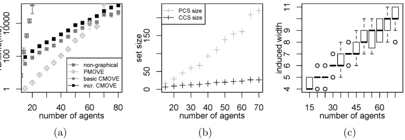
Figure 4: (a) Runtimes (ms) in log-scale for the nongraphical method, PMOVE and CMOVE with standard deviation of mean (error bars), (b) the corresponding number of vectors in the PCS and CCS, and (c) the corresponding spread of the induced width.
4.5.1 Random Graphs
To generate random MO-CoGs, we employ a procedure that takes as input: n, the number of agents;d, the number of payoff dimensions; ρ the number of local payoff functions; and
|Ai|, the action space size of the agents, which is the same for all agents. The procedure
then starts with a fully connected graph with local payoff functions connecting to two agents each. Then, local payoff functions are randomly removed, while ensuring that the graph remains connected, until only ρ local payoff functions remain. The values for the different objectives in each local payoff function are real numbers that are drawn independently and uniformly from the interval [0,10]. We compare algorithms on the same set of randomly generated MO-CoGs for each separate value ofn,d,ρ, and |Ai|.
To compare basic CMOVE, incremental CMOVE, PMOVE, and the non-graphical method, we test them on random MO-CoGs with the number of agents ranging between 10 and 85, the average number of factors per agent held at ρ = 1.5n, and the number of objectivesd= 2. This experiment was run on a 2.4 GHz Intel Core i5 computer, with 4 GB memory. Figure 4 shows the results, averaged over 20 MO-CoGs for each number of agents. The runtime (Figure 4a) of the non-graphical method quickly explodes. Both CMOVE variants are slower than PMOVE for small numbers of agents, but the runtime grows much more slowly than that of PMOVE. At 70 agents, both CMOVE variants are faster than PMOVE on average. For 75 agents, one of the MO-CoGs generated caused PMOVE to time out at 5000s, while basic CMOVE had a maximum runtime of 132s, and incremental CMOVE 136s. This can be explained by the differences in the size of the solutions, i.e., the PCS and the CCS (Figure 4b). The PCS grows much more quickly with the number of agents than the CCS does. For two-objective problems, incremental CMOVE seems to be consistently slower than basic CMOVE.
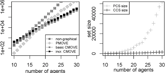
Figure 5: Runtimes (ms) for the non-graphical method, PMOVE and CMOVE in log-scale with the standard deviation of mean (error bars) (left) and the corresponding number of vectors in the PCS and CCS (right), for increasing numbers of agents and 5 objectives.
We therefore conclude that, in two-objective MO-CoGs, the non-graphical method is intractable, even for small numbers of agents, and that the runtime of CMOVE increases much less with the number of agents than PMOVE does.
To test how the runtime behavior changes with a higher number of objectives, we run the same experiment with the average number of factors per agent held at ρ = 1.5n and increasing numbers of agents again, but now ford= 5. This and all remaining experiments described in this section were executed on a Xeon L5520 2.26 GHz computer with 24 GB memory. Figure 5 (left) shows the results of this experiment, averaged over 85 MO-CoGs for each number of agents. Note that we do not plot the induced widths, as this does not change with the number of objectives. These results demonstrate that, as the number of agents grows, using CMOVE becomes key to containing the computational cost of solving the MO-CoG. CMOVE outperforms the nongraphical method from 12 agents onwards. At 25 agents, basic CMOVE is 38 times faster. CMOVE also does significantly better than PMOVE. Though it is one order of magnitude slower with 10 agents (238ms (basic) and 416ms (incremental) versus 33ms on average), its runtime grows much more slowly than that of PMOVE. At 20 agents, both CMOVE variants are faster than PMOVE and at 28 agents, Basic CMOVE is almost one order of magnitude faster (228s versus 1,650s on average), and the difference increases with every agent.
As before, the runtime of CMOVE is exponential in the induced width, which increases with the number of agents, from 3.1 at n= 10 to 6.0 atn = 30 on average, as a result of the random MO-CoG generation procedure. However, CMOVE’s runtime is polynomial in the size of the CCS, and this size grows exponentially, as shown in Figure 5 (right). The fact that CMOVE is much faster than PMOVE can be explained by the sizes of the PCS and CCS, as the former grows much faster than the latter. At 10 agents, the average PCS size is 230 and the average CCS size is 65. At 30 agents, the average PCS size has risen to 51,745 while the average CCS size is only 1,575.
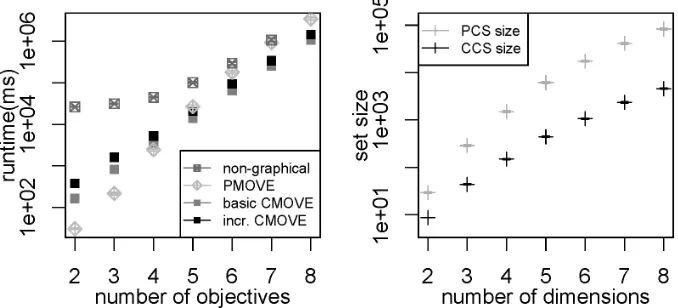
Figure 6: Runtimes (ms) for the non-graphical method, PMOVE and CMOVE in logscale with the standard deviation of mean (error bars) (left) and the corresponding number of vectors in the PCS and CCS (right), for increasing numbers of objectives.
several orders of magnitude slower at d = 2, grows slowly untild = 5, and then starts to grow with about the same exponent as PMOVE. This can be explained by the fact that the time it takes to enumerate of all joint actions and payoffs remains approximately constant, while the time it takes to prune increases exponentially with the number of objectives. When d= 2, CMOVE is an order of magnitude slower than PMOVE (163ms (basic) and 377 (incremental) versus 30ms). However, when d= 5, both CMOVE variants are already faster than PMOVE and at 8 dimensions they are respectively 3.2 and 2.4 times faster. This happens because the CCS grows much more slowly than the PCS, as shown in Figure 6 (right). The difference between incremental and basic CMOVE decreases as the number of dimensions increases, from a factor 2.3 at d= 2 to 1.3 at d = 8. This trend indicates that pruning after every cross-sum, i.e., at prune1, becomes (relatively) better for higher numbers of objectives. Although we were unable to solve problem instances with many more objectives within reasonable time, we expect this trend to continue and that incremental CMOVE would be faster than basic CMOVE for problems with very many objectives.
Overall, we conclude that, for random graphs, CMOVE is key to solving MO-CoGs within reasonable time, especially when the problem size increases in either the number of agents, the number of objectives, or both.
4.5.2 Mining Day
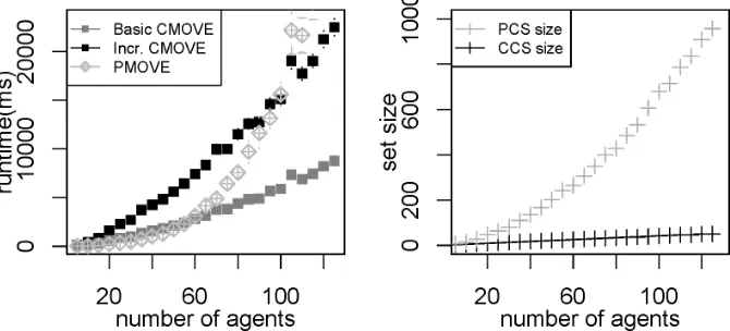
Figure 7: Runtimes (ms) for basic and incremental CMOVE, and PMOVE, in log-scale with the standard deviation of mean (error bars) (left) and the corresponding number of vectors in the PCS and CCS (right), for increasing numbers of agents.
the mining company wants to use the latest possible price information, and not lose time recomputing the optimal strategy with every price change. Therefore, we must calculate a CCS.
To generate a Mining Day instance with v villages (agents), we randomly assign 2-5 workers to each village and connect it to 2-4 mines. Each village is only connected to mines with a greater or equal index, i.e., if village iis connected to m mines, it is connected to minesitoi+m−1. The last village is connected to 4 mines and thus the number of mines isv+ 3. The base rates per worker for each resource at each mine are drawn uniformly and independently from the interval [0,10].
In order to compare the runtimes of basic and incremental CMOVE against PMOVE on a more realistic benchmark, we generate Mining Day instances with varying numbers of agents. Note that we do not include the non-graphical method, as its runtime mainly depends on the number of agents, and is thus not considerably faster for this problem than for random graphs. The runtime results are shown in Figure 7 (left). Both CMOVE and PMOVE are able to tackle problems with over 100 agents. However, the runtime of PMOVE grows much more quickly than that of CMOVE. In this two-objective setting, basic CMOVE is better than incremental CMOVE. Basic CMOVE and PMOVE both have runtimes of around 2.8sat 60 agents, but at 100 agents, basic CMOVE runs in about 5.9s and PMOVE in 21s. Even though incremental CMOVE is worse than basic CMOVE, its runtime still grows much more slowly than that of PMOVE, and it beats PMOVE when there are many agents.
5. Linear Support for MO-CoGs
In this section, we present variable elimination linear support (VELS). VELS is a new method for computing the CCS in MO-CoGs that has several advantages over CMOVE: for moderate numbers of objectives, its runtime complexity is better; it is an anytime
algorithm, i.e., over time, VELS produces intermediate results which become better and better approximations of the CCS and therefore, when provided with a maximum scalarized errorε, VELS can compute anε-optimal CCS.
Rather than dealing with the multiple objectives in the inner loop (like CMOVE), VELS deals with them in theouter loop and employs VE as a subroutine. VELS thus builds the CCS incrementally. With each iteration of its outer loop, VELS adds at most one new vector to a partial CCS. To find this vector, VELS selects a single w (the one that offers the maximal possible improvement), and passes thatwto the inner loop. In the inner loop, VELS uses VE (Section 2.2) to solve the single-objective coordination graph (CoG) that results from scalarizing the MO-CoG using the w selected by the outer loop. The joint action that is optimal for this CoG and its multi-objective payoff are then added to the partial CCS.
The departure point for creating VELS isCheng’s linear support (Cheng, 1988). Cheng’s linear support was originally designed as a pruning algorithm for POMDPs. Unfortunately, this algorithm is rarely used for POMDPs in practice, as its runtime is exponential in the number of states. However, the number of states in a POMDP corresponds to the number of objectives in a MO-CoG, and while realistic POMDPs typically have many states, many MO-CoGs have only a handful of objectives. Therefore, for MO-CoGs, the scalability in the number of agents is more important, making Cheng’s linear support an attractive starting point for developing an efficient MO-CoG solution method.
Building on Cheng’s linear support, in Section 5.1 we create an abstract algorithm that we call optimistic linear support (OLS), which builds up the CCS incrementally. Because OLS takes an arbitrary single-objective problem solver as input, it can be seen as a generic multi-objective method. We show that OLS chooses aw at each iteration such that, after a finite number of iterations, no further improvements to the partial CCS can be made and OLS can terminate. Furthermore, we bound the maximum scalarized error of the intermediate results, so that they can be used as bounded approximations of the CCS. Then, in Section 5.2, we instantiate OLS by using VE as its single-objective problem solver, yielding VELS, an effective MO-CoG algorithm.
5.1 Optimistic Linear Support
OLS constructs the CCS incrementally, by adding vectors to an initially emptypartial CCS:
Definition 13. A partial CCS, S, is a subset of the CCS, which is in turn a subset of V:
S ⊆CCS⊆ V.
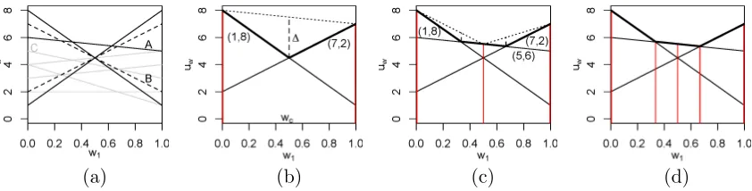
We define the scalarized value function over S, corresponding to the convex upper surface (shown in bold) in Figure 8b-d:
(a) (b) (c) (d)
Figure 8: (a) All possible payoff vectors for a 2-objective MO-CoG. (b) OLS finds two payoff vectors at the extrema (red vertical lines), a new corner weightwc= (0.5,0.5) is
found, with maximal possible improvement ∆. CCS is shown as the dotted line. (c) OLS finds a new vector at (0.5,0.5), and adds two new corner weights to Q. (d) OLS callsSolveCoGfor both corner weights (in two iterations), and finds no new vectors, ensuringS=CCS=CCS.
payoff vector inS:
u∗S(w) = max u(a)∈Sw
·u(a).
Similarly, we define the set of maximizing joint actions:
Definition 15. The optimal joint action set function with respect to S is a function that gives the joint actions that maximize the scalarized value:
AS(w) = arg max
u(a)∈S
w·u(a).
Note thatAS(w) is a set because for somewthere can be multiple joint actions that provide
the same scalarized value.
Using these definitions, we can describe optimistic linear support (OLS). OLS adds vectors to a partial CCS, S, finding new vectors for so-calledcorner weights. These corner weights are the weights where u∗S(w) (Definition 14) changes slope in all directions. These must thus be weights whereAS(w) (Definition 15) consists of multiple payoff vectors. Every
corner weight is prioritized by the maximal possible improvement of finding a new payoff vector at that corner weight. When the maximal possible improvement is 0, OLS knows that the partial CCS is complete. An example of this process is given in Figure 8, where the (corner) weights where the algorithm has searched for new payoff vectors are indicated by red vertical lines.
OLS is shown in Algorithm 7. To find the optimal payoff for a corner weight, OLS assumes access to a function called SolveCoG that computes the best payoff vector for a given w. For now, we leave the implementation of SolveCoG abstract. In Section 5.2, we discuss how to implementSolveCoG. OLS also takes as inputm, the MO-CoG to be solved, and ε, the maximal tolerable error in the result.
[image:25.612.99.520.93.200.2]Algorithm 7:OLS(m,SolveCoG, ε)
Input: A CoGG and an agentito eliminate.
1 S ← ∅//partial CCS,
2 W ← ∅//set of checked weights 3 Q←an empty priority queue
4 foreachextremum of the weight simplexwedo
5 Q.add(we,∞) // add extrema with infinite priority 6 end
7 while ¬Q.isEmpty()∧ ¬timeOut do 8 w←Q.pop()
9 u←SolveCoG(m,w) 10 if u6∈S then
11 Wdel←remove the corner weights made obsolete byufromQ, and store them 12 Wdel← {w} ∪Wdel//corner weights which are removed because of adding u 13 Wu←newCornerWeights(u, Wdel, S)
14 S←S∪ {u}
15 foreach w∈Wudo
16 ∆r(w)←calculate improvement usingmaxValueLP(w, S,W) 17 if ∆r(w)> εthen
18 Q.add(w, ∆r(w))
19 end
20 end
21 end
22 W ← W ∪ {w} 23 end
24 returnS and the highest∆r(w)left in Q
OLS prioritizes corner weights and how this can also be used to bound the error when stopping OLS before it is done finding a full CCS (Section 5.1.3).
5.1.1 Initialization
OLS starts by initializing the partial CCS, S, which will contain the payoff vectors in the CCS discovered so far (line 1 of Algorithm 7), as well as the set of visited weightsW (line 2). Then, it adds the extrema of the weight simplex, i.e., those points where all of the weight is on one objective, to a priority queue Q, with infinite priority (line 5).
These extrema are popped off the priority queue when OLS enters the main loop (line 7), in which the w with the highest priority is selected (line 8). SolveCoG is then called withw (line 9) to findu, the best payoff vector for thatw.
For example, Figure 8b shows S after two payoff vectors of a 2-dimensional MO-CoG have been found by applying SolveCoG to the extrema of the weight simplex: S =
5.1.2 Corner Weights
After having evaluated the extrema,Sconsists ofd(the number of objectives) payoff vectors and associated joint actions. However, for many weights on the simplex, it does not yet contain the optimal payoff vector. Therefore, after identifying a new vectoru to add to S (line 9), OLS must determine what new weights to add to Q. Like Cheng’s linear support, OLS does so by identifying the corner weights: the weights at the corners of the convex upper surface, i.e., the points where the PWLC surface u∗S(w) changes slope. To define the corner weights precisely, we must first define P, the polyhedral subspace of the weight simplex that is above u∗S(w) (Bertsimas & Tsitsiklis, 1997). The corner weights are the vertices of P, which can be defined by a set of linear inequalities:
Definition 16. If S is the set of known payoff vectors, we define a polyhedron
P ={x∈ <d+1:S+x≥~0,∀i, wi >0,
X
i
wi = 1},
where S+ is a matrix with the elements of S as row vectors, augmented by a column vector
of −1’s. The set of linear inequalitiesS+x≥~0, is supplemented by the simplex constraints:
∀i wi > 0 and Piwi = 1. The vector x = (w1, ..., wd, u) consists of a weight vector and
a scalarized value at those weights. The corner weights are the weights contained in the vertices ofP, which are also of the form (w1, ..., wd, u).
Note that, due to the simplex constraints, P is only d-dimensional. Furthermore, the extrema of the weight simplex are special cases of corner weights.
After identifying u, OLS identifies which corner weights change in the polyhedronP by adding u toS. Fortunately, this does not require recomputation of all the corner weights, but can be done incrementally: first, the corner weights in Q for which u yields a better value than currently known are deleted from the queue (line 11) and then the function newCornerWeights(u, Wdel, S) at line 13 calculates the new corner weights that involve u
by solving a system of linear equations to see where u intersects with the boundaries and the relevant subset of the present vectors in S.
newCornerWeights(u, Wdel, S) (line 13) first calculates the set of all relevant payoff
vectors,Arel, by taking the union of all the maximizing vectors of the weights in Wdel9:
Arel=
[
w∈Wdel
AS(w).
If any AS(w) contains fewer than dpayoff vectors, then a boundary of the weight simplex
is involved. These boundaries are also stored. All possible subsets of sized−1 (of vectors and boundaries) are taken. For each subset the weight where these d−1 payoff vectors (and/or boundaries) intersect with each other and u is computed by solving a system of linear equations. The intersection weights for all subsets together form the set of candidate corner weights: Wcan. newCornerWeights(u, Wdel, S) returns the subset ofWcan which are
inside of the weight simplex and for whichu has a higher scalarized value than any payoff
vector already in S. Figure 8b shows one new corner weight labelled wc = (0.5,0.5). In
practice,|Arel|is very small, so only a few systems of linear equations need to be solved.10
After calculating the new corner weights Wu at line 13, u is added to S at line 14. Cheng showed that finding the best payoff vector for each corner weight and adding it to the partial CCS, i.e., S←S∪ {SolveCoG(w)}, guarantees the best improvement toS:
Theorem 8. (Cheng 1988) The maximum value of:
max
w,u∈CCSminv∈Sw·u−w·v,
i.e., the maximal improvement toS by adding a vector to it, is at one of the corner weights (Cheng, 1988).
Theorem 8 guarantees the correctness of OLS: after all corner weights are checked, there are no new payoff vectors; thus the maximal improvement must be 0 and OLS has found the full CCS.
5.1.3 Prioritization
Cheng’s linear support assumes that all corner weights can be checked inexpensively, which is a reasonable assumption in a POMDP setting. However, since SolveCoGis an expensive operation, testing all corner weights may not be feasible in MO-CoGs. Therefore, unlike Cheng’s linear support, OLS pops only one w off Q to be tested per iteration. Making OLS efficient thus critically depends on giving each w a suitable priority when adding it toQ. To this end, OLS prioritizes each corner weight waccording to its maximal possible improvement, an upper bound on the improvement inu∗S(w). This upper bound is computed with respect to CCS, the optimistic hypothetical CCS, i.e., the best-case scenario for the final CCS given that S is the current partial CCS and W is the set of weights already tested withSolveCoG. The key advantage of OLS over Cheng’s linear support is that these priorities can be computed without calling SolveCoG, obviating the need to runSolveCoG on all corner weights.
Definition 17. An optimistic hypothetical CCS, CCS is a set of payoff vectors that yields the highest possible scalarized value for all possible w consistent with finding the vectors S
at the weights in W.
Figure 8b denotes the CCS={(1,8),(7,2),(7,8)} with a dotted line. Note thatCCS is a superset of S and the value of u∗CCS(w) is the same asu∗S(w) at all the weights inW. For a givenw,maxValueLP finds the the scalarized value ofu∗
CCS(w) by solving:
max w·v
subject to W v≤u∗S,W,
whereu∗S,W is a vector containing uS∗(w0) for allw0∈ W. Note that we abuse the notation
W, which in this case is a matrix whose rows consist of all the weight vectors in the set
W.11
UsingCCS, we can define the maximal possible improvement:
∆(w) =u∗CCS(w)−u∗S(w).
Figure 8b shows ∆(wc) with a dashed line. We use themaximal relative possible
improve-ment, ∆r(w) = ∆(w)/u∗CCS(w), as the priority of each new corner weight w ∈ Wu. In
Figure 8b, ∆r(wc)=(0.5,0.5)·((77.5,8)−(1,8))= 0.4.When a corner weightwis identified (line 13),
it is added toQwith priority ∆r(w) as long as ∆r(w)> ε(lines 16-18).
After wc in Figure 8b is added to Q, it is popped off again (as it is the only element
of Q). SolveCoG(wc) generates a new vector (5,6), yielding S = {(1,8),(7,2),(5,6)}, as
illustrated in Figure 8c. The new corner weights (0.667,0.333) and (0.333,0.667) are the points at which (5,6) intersects with (7,2) and (1,8). Testing these weights, as illustrated in Figure 8d, does not result in new payoff vectors, causing OLS to terminate. The maximal improvement at these corner weights is 0 and thus, due to Theorem 8, S = CCS upon termination. OLS called solveCoG for only 5 weights resulting exactly in the 3 payoff vectors of the CCS. The other 7 payoff vectors in V (displayed as grey and dashed black lines in Figure 8a) were never generated.
5.2 Variable Elimination Linear Support
Any exact CoG algorithm can be used to implement SolveCoG. A naive approach is to explicitly compute the values of all joint actionsVand select the joint action that maximizes this value:
SolveCoG(m,w) = arg max u(a)∈V
w·u(a).
This implementation of SolveCoG in combination with OLS yields an algorithm that we refer to asnon-graphical linear support (NGLS), because it ignores the graphical structure, flattening the CoG into a standard multi-objective cooperative normal form game. The main downside is that the computational complexity of SolveCoG is linear in |V| (which is equal to |A|), which is exponential in the number of agents, making it feasible only for MO-CoGs with very few agents.
By contrast, if we use VE (Section 2.2) to implement SolveCoG, we can do better. We call the resulting algorithm variable elimination linear support (VELS). Having dealt with the multiple objectives in the outer loop of OLS, VELS relies on VE to exploit the graphical structure in the inner loop, yielding a much more efficient method than NGLS.
5.3 Analysis
We now analyze the computational complexity of VELS.
11. Our implementation of OLS reduces the size of the LP by using only the subset of weights inW for which the joint actions involved in w,AS(w), have been found to be optimal. This can lead to a slight