Finite Element Technology for Gradient Elastic Fracture Mechanics

Procedia Materials Science 3 ( 2014 ) 2042 – 2047

2211-8128 © 2014 Elsevier Ltd. Open access under CC BY-NC-ND license.

Selection and peer-review under responsibility of the Norwegian University of Science and Technology (NTNU), Department of Structural Engineering doi: 10.1016/j.mspro.2014.06.329

ScienceDirect

20th European Conference on Fracture (ECF20)

Finite element technology for gradient elastic fracture mechanics

Cristian Bagni

*, Harm Askes

, Luca Susmel

a_{University of Sheffield, Department of Civil and Structural Engineering, Mappin Street, Sheffield S1 3JD, United Kingdom}

Abstract

In this paper a unified FE methodology based on gradient-elasticity is presented, including Gauss integration rules and error estimation. Applying the proposed methodology to classical elasticity problems, it has been found that, the linear elements show a convergence rate higher than the theoretical one, for what concerns the stresses. This means that, accepting a small loss in the accuracy of the solution, the use of linear elements, instead of quadratic elements, leads to a solution characterised by a convergence rate higher than the theoretical one along with a sensible reduction in the computational cost. This technology has many possible applications such as the simulation of fatigue failure and bone regeneration.

© 2014 The Authors. Published by Elsevier Ltd.

Selection and peer-review under responsibility of the Norwegian University of Science and Technology (NTNU), Department of Structural Engineering.

Keywords: gradient elasticity, fracture mechanics, length scale, bone regeneration.

1.Introduction

In recent years, elasticity formulations have been used at the micro and nanostructure level and it is exactly at these scales that experimental observations have shown that classical continuum theories fail in the accurate description of deformation phenomena. Furthermore, classical elastic singularities at dislocation lines and crack tips hamper interpretation of the structural response.

* Corresponding author.

E-mail address: c.bagni@sheffield.ac.uk

© 2014 Elsevier Ltd. Open access under CC BY-NC-ND license.

Nomenclature

C elasticity matrix

K stiffness matrix

Nu, Nσ shape functions matrix (for displacements and stresses) Bu strain-displacement matrix

b body forces

f force vector

uc_{, d}c _{continuum and nodal classical elasticity displacements}

g

ı continuum nonlocal stress tensor

sg _{nodal nonlocal stress tensor}

A length scale

The reason why classical continuum theories fail in the description of the problems mentioned above is the lack, in the constitutive equations, of an internal length, representative of the underlying microstructure. To overcome these deficiencies, it has been proposed to enrich the constitutive equations of classical elasticity by including high-order gradients of particular state variables (e.g. strain or stress), multiplied by internal lengths (see for instance Askes and Aifantis (2011) for an historical overview of these formulations).

Since for the most part of the engineering problems a numerical solution is needed, implementation of gradient elasticity is of central importance. Here, the finite element method will be used. Until now, due to the non-standard finite element implementation of gradient elasticity, these theories have been applied to a limited number of finite elements (usually mono-dimensional or linear quadrilateral elements) and without any knowledge about optimal interpolation and integration rules. The aim of this paper is to present a unified FE methodology based on gradient-elasticity, and in particular on the Ru-Aifantis theory (Aifantis (1992); Altan and Aifantis (1992); Ru and Aifantis (1993)), valid for both two- and three-dimensional finite elements, along with Gauss integration rules and error estimation.

2.Shape functions and finite element equations

Discretisation of the displacements has been performed through the traditional shape functions Ni which are collected in a matrixNu that for 2D elements can be written as:

» ¼ º « ¬ ª = " " 2 1 2 1 u 0 0 0 0 N N N N

N (1)

Once the nodal displacements d = [d1x, d1y, d2x, d2y, …]T are known, the continuum displacements u = [ux, uy]T

can be determined through the relation u=Nud. Moreover, the derivative operators ∇and L have been defined as

» » » » ¼ º « « « « ¬ ª ∂ ∂ ∂ ∂ = ∇ y

x with _∇2_=∇T_{∇ and}

T 0 0 » » » » ¼ º « « « « ¬ ª ∂ ∂ ∂ ∂ ∂ ∂ ∂ ∂ = x y y x

L (2)

As explained in Askes and Aifantis (2011), the Ru-Aifantis theorem splits the original fourth-order partial differential equations (p.d.e.) into two sets of second-order p.d.e., which allows us to determine, in first instance, the local displacements _uc _{by solving the p.d.e. of classical elasticity:}

0 b CLu

Taking the weak form of Eq. (3), followed by integration by parts and using the finite element discretisation described above, Eq. (3) leads to

f Kd d CB

B Ω ≡ =

³

c c

T _d

u

u (4)

where Bu=LNu and f collects the contributions of both the body forces and the external loads.

Then, with a second set of equations it is possible to evaluate the gradient-enriched strain or stress field. For what concerns the stress-based theory, in the second step the gradient activity is introduced by using the displacements of the classical elasticity equations as a source term in

(

)

ı

ı −A2∇2 = (5)

Considering again the weak form of Eq. (5) and integrating by part, we obtain

(

)

_³

³

³

¼ º « « ¬ ª ¸ ¸ ¹ · ¨ ¨ © § ∂ ∂ ∂ ∂ + ∂ ∂ ∂ ∂

+ d d d

y y x x c g g g

g _{w CLu}

ı n w ı w ı w ı

w T 2 T

T T

2 T

A

A (6)

where n = [nx, ny]T contains the components of the normal vector to the boundary ī and w is the test function vector.

Ignoring for the moment the boundary term and adopting, for the discretisation, an expanded form Nσof the

shape function matrix Nu given in Eq. (1), in order to accommodate all the three nonlocal stress components, through which ıg =Nσsg, using the same shape functions Nσ to discretise w and with uc =Nudc, the resulting system of equations reads

c u g

T _{d d}

y y x

x s N CB d

N N N N N N

_³

³

º « « ¬ ª ¸ ¸ ¹ · ¨ ¨ © § ∂ ∂ ∂ ∂ + ∂ ∂ ∂ ∂

+ 2 T T T

σ σ σ σ σ σ

σ A (7)

The shape functions Nσ can be defined independently from Nu, but it is most convenient to use the same finite element discretisation for Eqs. (4) and (7).

3.Numerical integration

To solve the first and second step of the Ru-Aifantis theory described above (i.e. Eqs. (4) and (7)) the Gauss quadrature rule has been adopted.

Table 1. Number of Gauss points used in the first step of the Ru-Aifantis theory.

Elements Order Gauss Points

Triangles Linear 1

Quadratic 3

Quadrilaterals Bi-linear 2x2

Bi-quadratic 2x2

Since the first step of the Ru-Aifantis theory consists in the solution of the second-order p.d.e. of classical elasticity, for the numerical integration of the stiffness matrix K, the usual number of integration points is used for each kind of implemented elements, as summarised in Table 1.

both A₌0 and A_≠0. Obviously this possibility would be extremely desirable, but unfortunately it is not always verified, as described afterwards.

We will use M to denote the first matrix term of the left integral in Eq. (7) and D the second one, i.e.

σ σN N

M₌ T _and

y y x x

T T

∂ ∂ ∂ ∂ + ∂ ∂ ∂ ∂

= Nσ Nσ Nσ Nσ

D (8)

The investigation has been carried out through a study of the eigenvalues of the matrix M_+A2D _{when A≠0}

and, obviously, of the matrix M on its own when A=0; in particular, to avoid rank deficiencies all the eigenvalues must be non-zero, which means that zero energy modes are not admitted.

From the performed studies it turned out that, when A=0, it is possible to use the same integration rule only for the linear quadrilateral elements, while for the other three type of elements higher order integration rules are needed (the minimum number of integration points is given in Table 2, for each kind of element). On the contrary, for A≠0 , due to the contribution of the matrix D, it is possible to use the same integration rule, used in the first step, for every type of finite element.

Table 2. Number of Gauss points used in the second step of the Ru-Aifantis theory.

Elements Order Gauss Points

Triangles Linear 3

Quadratic 6 (degree of precision 4)

Quadrilaterals Bi-linear 2x2

Bi-quadratic 3x3

4.Error estimation and convergence study

With the most suitable integration rules for each kind of finite element now identified, the attention has been focused on the error estimation of the new methodology and in particular the convergence rate of the different finite elements has been studied for some simple classical elasticity problems, an example is presented in 4.1.

To determine the convergence rate, the L2-norm error defined as

e c e e

σ σ σ − =

2 (9)

where σe and σc are, respectively, the exact and calculated values of the stresses, has been plotted against the number of degrees of freedom (nDoF).

From the theory it is well known that the errors on displacements and stresses are proportional to the nDoF, respectively, as

(

)

2 1 n

nDoF O nDoF

O _¸¸=

¹ · ¨

¨ © §

≈

+ −

u

e and 2

(

)

n

nDoF O nDoF

O _¸¸=

¹ · ¨

¨ © §

≈ −

ı

e (10)

where n is the polynomial order.

From Eq. (10), it is clear that the

||

||

Fig. 1. Cylinder subject to an internal pressure (left), mode I fracture problem (right): geometry and loading conditions.

4.1.Cylinder subject to internal pressure

One of the analysed problems is the case of a cylinder subjected to an internal pressure pi shown in Fig. 1. The geometrical and material parameters of the problem are b₌4m, a=1m, _E=109_N/m2_{, Ȟ=0.25 and A=0mm.}

An internal pressure pi =107N/m2 is applied.

Thanks to the symmetry of the problem only a quarter of the vessel has been modelled. The domain has been modelled with all four types of implemented finite elements, starting from a rough mesh and performing then a mesh refinement. For what concerns the triangular elements different meshes has been tested: one without symmetry and 2 characterised by different symmetries (only 1 for the quadratic elements). The boundary conditions are taken as homogeneous essential so that the circumferential displacements uθ are null along the two axes of symmetry.

Fig. 2. Cylinder subject to internal pressure: displacements (left)/stress (right) error versus number of Degrees of Freedom.

To define the error, the numerical solutions, obtained using the new methodology, have been compared with the exact solution of the problem available in Timoshenko and Goodier (1970).

As shown in Fig. 2, while for the quadratic elements the convergence rate is nearly equal to the theoretical one, for the linear elements the convergence rate, obtained applying the new methodology, is higher than the theoretical one for what concerns the stresses; the opposite is true regarding the displacements. This is an extremely interesting and powerful result for stress estimation, especially from the commercial point of view, because accepting a small loss in the accuracy of the solution, the use of the linear elements leads to a solution characterised by a higher convergence rate, along with a sensible reduction in the computational cost, compared with the quadratic elements.

5.Application

0.25

Ȟ= and A₌0.1mm. Prescribed displacements u₌0.01mmare applied at the top and bottom edges. Due to the symmetry only the top-right quarter has been modelled and in particular with 32x32 bi-linear and biquadratic quadrilateral elements and with the double of linear and quadratic triangular elements.

The boundary conditions accompanying Eq. (6) are taken as both homogeneous natural throughout the domain 0)

ı

(n g

m kl, 2

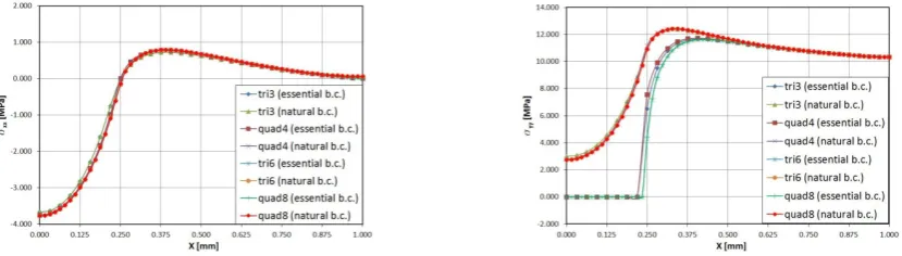
mA = and homogeneous essential, that is the nonlocal stresses components are prescribed so that σxx=0 on the vertical edges, σyy=0 on the face of the crack and σxy=0everywhere. In Fig. 3 σxx and σyy, obtained

with both the boundary conditions, are plotted and compared; it can be seen that the application of the different boundary conditions produces almost no variations for σxx and moderate effects on σyy.

Fig. 3. Mode I fracture problem: comparison of the ıxx (left) and ıyy (right) values for y = 0, obtained with the different types of finite elements.

6.Conclusions

In this paper a unified FE methodology based on gradient-elasticity, for two-dimensional finite elements, has been presented, including Gauss integration rules and error estimation.

The proposed methodology has been applied to classical elasticity problems and it has been found that, for what concerns the stress evaluation, while for the quadratic elements the convergence rate is nearly equal to the theoretical one, the linear elements show a convergence rate higher than the theoretical one. This is an extremely important result, especially from the commercial point of view, because accepting a small loss in the accuracy of the solution, the use of linear elements, instead of quadratic elements, leads to a solution characterised by a convergence rate higher than the theoretical one along with a sensible reduction in the computational cost.

Furthermore, the proposed methodology has been applied to a mode I fracture problem, showing that the different finite elements produce comparable results (as expected) and that singularities in the stress field are removed; the application of different boundary conditions has been also investigated.

At the moment, the methodology for three-dimensional finite elements is under implementation.

Future applications of this new methodology will focus on the simulation of fatigue failure and bone regeneration.

Acknowledgements

Financial support from Safe Technology Ltd is gratefully acknowledged.

References

Aifantis, E.C., 1992. On the role of gradients in the localization of deformation and fracture. Int. J. Eng. Sci. 30, 1279-1299. Altan, S., Aifantis, E.C., 1992. On the structure of the mode III crack-tip in gradient elasticity. Scripta Metall. Mater. 26, 319-324.

Askes, H., Aifantis, E., 2011. Gradient elasticity in statics and dynamics: An overview of formulations, length scale identification procedures, finite element implementations and new results. Int. J. Solids Struct. 48, 1962–1990.