Linear multivariate evaluation models for spatial perception of soundscape

White Rose Research Online URL for this paper: http://eprints.whiterose.ac.uk/91513/

Version: Accepted Version

Article:

Deng, Z., Kang, J., Wang, D. et al. (2 more authors) (2015) Linear multivariate evaluation models for spatial perception of soundscape. Journal of the Acoustical Society of America, 138 (5). pp. 2860-2870. ISSN 0001-4966

https://doi.org/10.1121/1.4934272

[email protected] https://eprints.whiterose.ac.uk/ Reuse

Unless indicated otherwise, fulltext items are protected by copyright with all rights reserved. The copyright exception in section 29 of the Copyright, Designs and Patents Act 1988 allows the making of a single copy solely for the purpose of non-commercial research or private study within the limits of fair dealing. The publisher or other rights-holder may allow further reproduction and re-use of this version - refer to the White Rose Research Online record for this item. Where records identify the publisher as the copyright holder, users can verify any specific terms of use on the publisher’s website.

Takedown

If you consider content in White Rose Research Online to be in breach of UK law, please notify us by

Z. Deng, J. Kang, D. Wang, A. Liu & J. Z. Kang: J. Acoust. Soc. Am. [DOI: 10.1121/1.4934272]

Journal of Acoustical Society of America, Volume 138(5), November 2015, Pages: 2860-2870 Page1 / 17

Linear multivariate evaluation models for spatial

perception of soundscape

Zhiyong Denga*, Jian Kangb, Daiwei Wanga, Aili Liuc, Joe Zhengyu Kangd

a

Music College, Capital Normal University, No.105 Xisanhuan, Beijing, China, 100048

b

School of Architecture, University of Sheffield, Sheffield, United Kingdom

c

College of Resource Environment and Tourism, Capital Normal University, Beijing, China

d_{The Queen’s College}

, University of Oxford, Oxford, UK

* Corresponding author

ABSTRACT: Soundscape is a sound environment that emphasizes the awareness of auditory

perception and social or cultural understandings. The case of spatial perception is significant to soundscape. However, previous studies on the auditory spatial perception of the soundscape environment have been limited. Based on 21 native binaural-recorded soundscape samples and a set of auditory experiments for subjective spatial perception (SSP), a study of the analysis among semantic parameters, the inter-aural-cross-correlation coefficient (IACC), A-weighted-equal sound-pressure-level (Leq), dynamic (D) and SSP is introduced to verify the

independent effect of each parameter and to re-determine some of their possible relationships. The results show that the more noisiness the audience perceived, the worse spatial awareness they received, while the closer and more directional the sound source image variations, dynamics and numbers of sound sources in the soundscape are, the better the spatial awareness would be. Thus, the sensations of roughness, sound intensity, transient dynamic and the values of Leq and IACC have a suitable range for better spatial perception. A better spatial awareness

seems to promote the preference slightly for the audience. Finally, setting SSPs as functions of the semantic parameters and Leq-D-IACC, two linear multivariate evaluation models of

subjective spatial perception are proposed.

Keywords: Spatial perception, Binaural-recorded, IACC, Semantic parameter

PACS numbers: _{43.50.Rq; 43.50.Qp, 43.55.Cs, 43.66.Lj}

1. Introduction

Soundscape, which was previously proposed by Canadian composer and ecologist Schafer in the 1970s, is a sound environment that emphasizes human awareness of their auditory perceptions or social and cultural understandings. Soundscape, as defined by Schafer, includes three main factors: audience, environment and a sound event with the features of keynote, sound signal and soundmark [1].

In the case of human awareness, sound spatial perceptions are defined as a general auditory awareness of the three-dimensional sound spaces, locations and variations [2]. Because soundscape cannot be isolated from the landscape [3, 4], it is always significant to

a)

soundscape. During the 1950s, inter-aural level difference (ILD) and inter-aural time difference (ITD) were mechanisms for sound localizations [5, 6], and then binaural impulse response was proposed by Schroeder [7] to examine the sound quality of room acoustics. With the development of binaural recording technology, the inter-aural cross-correlation coefficient (IACC) was suggested as an independent acoustic parameter to evaluate sound spatial perceptions of a concert hall [2], and some relationships between room acoustics and psychoacoustics were found based on further study of the IACC [8, 9]. Around 2000, still based on the IACC, a model of the auditory brain system proposed by Ando was suggested to describe the primitive temporal and spatial factors for some spatial sensations, such as localization in the horizontal plane of sound fields [10, 11, 12]. Recently, the head-related transfer function (HRTF) and inter-aural cross-correlation function (IACF) were used to create the spatial awareness of virtual audio environments and sound playback systems [13, 14, 15]. However, previous studies on sound spatial perception of open space and soundscape environments were limited, and few efficient predictive models were introduced. According to some of the newest studies regarding the spatiotemporal variability of soundscapes [16], soundwalk [17], listening behaviors in public space [18, 19] and the evaluations of acoustic and cultural awareness for historical soundscape environments [20, 21, 22], physical acoustic parameters alone, such as A-weighted equal sound pressure level (Leq), IACC or dynamic (D)

defined as the maximum difference of sound pressure level during the amplitude variations of a sound signal [21], are not efficient for predicting a more complicated spatial perception of the soundscape or real urban and rural public sound space.

Thus, based on 21 typical native binaural-recorded soundscape samples and a set of auditory experiments for the subjective spatial perceptions, the aim of this study is to verify the independent effect on subjective spatial perceptions (SSPs) of semantic parameters and three well-known and simple-measured acoustic parameters, IACC, Leq (dBA) and D

(dynamic); re-determine some of their possible relationships; and finally propose two linear multivariate evaluation models of subjective spatial perceptions, taking into account SSPs as functions of the semantic parameters and Leq-D-IACC.

2. Methods

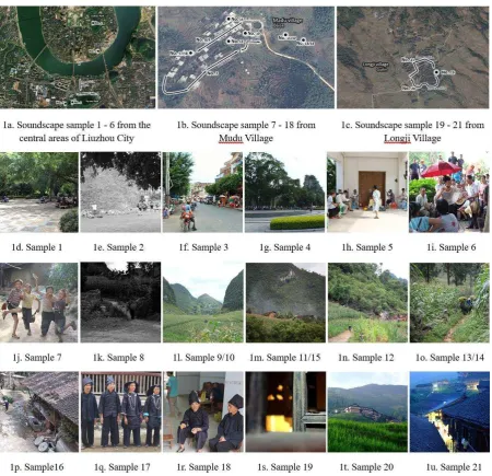
2.1 Study areas and samples

Z. Deng, J. Kang, D. Wang, A. Liu & J. Z. Kang: J. Acoust. Soc. Am. [DOI: 10.1121/1.4934272]

Journal of Acoustical Society of America, Volume 138(5), November 2015, Pages: 2860-2870 Page3 / 17

Fig. 1. The native locations and situations of 21 soundscape samples

2.2 Binaural recording technology

The binaural-recorded signals typically come from two small omni-directional microphones, which are located in the ear canal of a human head or dummy head. When played through a pair of stereo earphones or headphones, a binaural-recorded sound signal could represent the spatial information around the head of the audience, mainly including the sound image locations and their variations with SPL variations. Binaural recording technology was previously used to examine the binaural impulse response of room acoustics6. It is easy to acquire another important acoustic parameter, IACC, from binaural-recorded samples by using Equation (1), while the IACF can be acquired as shown in Equation (2).

as far as possible for stationary recorded samples, and for the sound walking samples, it was kept along with the forward direction of the walking path. The fixed directions of the stationary samples and walking paths of the sound walking samples were based on the situation of environment and the recommendation of local people. The “stationary” or “sound walking” status of each sample is listed in the last column of Table 2.

In this paper, all of the binaural-recorded samples are digitized with a 44.1 kHz sampling rate. Due to the possible maximum distance of the two eardrums, the delay time between the two eardrums is in the range of -44 samples to 44 samples because the aural sound images on the left and right hemispheres are approximately symmetric, especially in the middle frequency and low frequency8. The delay time , represented by the sample numbers, should be set in a range of 0 to 44 samples. Then, according to Equation (2), the variegated IACF curves of the 21 samples are shown normally in Fig. 3.

) ( max

2 1t



IACF

IACC  (1)







t L R

t t dt t p dt t p dt t p t p IACF   (2)

- pL, the sound pressure received by the left ear, represented by the voltage level of the left channel;

- pR, the sound pressure received by the right ear, represented by the voltage level of the right channel;

- , the delay time between two ears, represented by the sample numbers in a digitalized sound signal.

Fig. 2. Sound pressure level envelopes of samples Fig. 3. IACF curves of samples

2.3 Auditory experiment and semantic parameters

Z. Deng, J. Kang, D. Wang, A. Liu & J. Z. Kang: J. Acoust. Soc. Am. [DOI: 10.1121/1.4934272]

Journal of Acoustical Society of America, Volume 138(5), November 2015, Pages: 2860-2870 Page5 / 17

Table 1. Semantic parameters measurement questionnaire

No. Semantic parameter and code

5-point Likert scale

-2 -1 0 1 2

1

QN (Quiet – Noisy)

BL (Boring – Lively)

RS (Rough – Smooth)

DO (Directive – Omni)

CF (Close – Far)

WS (Weak – Strong)

SIV (Sound image variation, Less - More) TrD (Transient Dynamic, Low - High) NSS (Number of sound sources, Less - More)

SPA (Subjective preferred assessment, Don’t like - Like)

SSP (Subjective spatial perceptions, Low – High)

All samples were binaural-recorded sounds and played back through a standard stereo headphone system with sound pressure levels consistent with the values of Leq in TABLE II

and an interval of 10 s between each sound. The duration of each soundscape sample was from 26 s to 239 s.

2.4 Statistical analysis

Pearson correlation analysis was used to examine the possible relationships among the semantic parameters, IACC, Leq (dBA), D (dynamic) and the SSP. Then, the SSP was set as

the controlling variable, and principal components analysis and system clustering analysis were applied to determine the interaction influence of QN, BL, RS, DO, CF, WS, SIV, TrD, NSS and SPA, as well as to find the orthogonal principal components of the SSP. Finally, multi-regression was used to create the linear single-value evaluation models of the SSP. All of the statistics mentioned above were carried out in MATLAB® 2012a, SPSS® 20.0 and Excel® 2013.

3. Results, Analysis and Models

3.1 Correlation analysis

According to the results of the auditory experiment, the average values of the semantic parameters (QN, BL, RS, DO, CF, WS, SIV, NSS, SPA and the SSP), IACC, Leq and

descriptions of the soundscape contents are shown in Table 2. The correlations are shown in Table 3.

the lowest correlation with the subjective spatial perception (SSP), i.e., 0.019 and 0.006, respectively, which are close to zero. Moreover, in the cases of the three important acoustic parameters, i.e., IACC, Leq and D (dynamic), the highest correlation value (i.e., 0.621) exists

between D (dynamic) and SSP, while the other ones show a similarity for the absolute values of -0.193 and 0.205.

Table 2. Semantic and acoustic parameter values of the soundscape samples

No.

Average value of semantic parameters Acoustic

parameters

Soundscape

description

Status of

recorded

position

QN BL RS DO CF WS SIV TrD NSS SPA SSP IACC Leq

(dBA) D

(dB)

1 0.54 0.92 0.00 -0.29 0.00 -0.21 1.29 0.17 0.71 0.75 0.75 0.22 65 37 Tango in Liuhou Park. Stationary

2 1.46 -0.63 -0.83 0.33 -0.83 0.88 0.29 0.83 0.63 -0.83 -0.83 0.18 65 33 Elderly people activities. Stationary

3 1.67 -0.33 -0.50 -0.42 -0.71 0.88 0.96 0.71 0.71 -0.38 -0.38 0.09 73 26 Guangming Road Market. Sound walking

4 1.38 -0.21 -0.29 -0.33 -0.79 0.88 0.79 0.58 0.21 -0.46 -0.46 0.31 74 27 Yu-ma Park soundscape. Sound walking

5 0.79 0.29 0.08 0.17 -1.04 0.83 -0.21 0.50 -0.04 0.00 0.00 0.26 85 5 Small folk orchestra with Stationary

6 0.38 0.54 0.00 -0.04 -0.83 0.54 0.50 0.63 0.75 0.17 0.17 0.23 75 31 Three antiphonal singing. Stationary

7 -0.42 1.38 0.79 -0.71 -0.75 0.08 1.04 0.63 0.54 1.21 1.21 0.14 72 46 Village dusk soundscape. Sound walking

8 -1.17 0.54 0.63 -0.33 -0.17 -0.71 -0.21 -0.25 -0.50 0.13 0.13 0.27 55 36 Village night soundscape. Sound walking

9 -1.38 0.63 0.75 -0.04 -0.08 -0.50 0.13 -0.33 0.17 0.33 0.33 0.33 60 35 Village morning, sound. Sound walking

10 -1.71 0.67 1.13 1.00 0.79 -1.29 -1.04 -0.96 -0.33 0.54 0.54 0.05 40 11 Village morning, quiet. Sound walking

11 -1.38 0.46 0.71 0.54 0.50 -0.92 -1.04 -0.71 -0.58 0.29 0.29 0.04 48 9 Village sound with insects. Stationary

12 -0.88 0.42 0.25 0.04 -0.67 -0.63 -0.38 -0.29 -0.25 0.25 0.25 0.12 55 25 Village sound of working. Sound walking

13 -1.21 0.17 0.25 0.25 -0.67 0.13 -0.25 0.46 0.25 0.54 0.54 0.96 75 46 Talk among local people. Stationary

14 -0.38 0.38 0.33 0.29 -0.58 -0.33 -0.46 0.13 -0.46 0.13 0.13 0.60 69 12 Village sound in farmland. Sound walking

15 -0.29 0.42 -0.08 0.58 -0.92 0.13 -0.38 0.33 0.08 0.13 0.13 0.67 75 37 Village sound with birds. Stationary

16 0.00 0.75 0.29 0.58 -1.38 0.67 0.17 0.67 -0.04 0.58 0.58 0.76 76 13 Village sound with crowing. Sound walking

17 0.25 0.46 0.38 0.17 -1.21 0.75 -0.67 0.54 -0.13 0.38 0.38 0.22 79 21 Antiphonal singing. Stationary

18 0.75 0.33 -0.29 -0.50 -1.42 1.04 0.63 0.63 0.75 0.04 0.04 0.15 70 52 Interviews for the singers. Stationary

19 -0.75 -0.04 0.25 -0.04 0.04 -0.71 -0.29 -0.50 -0.04 -0.21 -0.21 0.27 50 17 Village soundscape indoors. Stationary

20 0.63 -0.63 -0.29 0.00 -0.42 0.38 0.54 0.33 0.38 -0.54 -0.54 0.59 70 35 Valley sound walking. Sound walking

Table 3. Correlation coefficients among the subjective spatial perception parameters

Parameters QN BL RS DO CF WS SIV TrD NSS IACC Leq (dBA) D SPA SSP

NQ 1

BL -0.517 1

RS -0.857 0.714 1

DO -0.357 -0.058 0.260 1

CF -0.593 0.107 0.536 0.265 1

WS 0.861 -0.370 -0.744 -0.314 -0.854 1

SIV 0.643 -0.047 -0.523 -0.750 -0.344 0.538 1

TrD 0.794 -0.234 -0.682 -0.350 -0.859 0.935 0.613 1

NSS 0.656 -0.181 -0.620 -0.504 -0.394 0.631 0.832 0.674 1

IACC -0.071 -0.129 -0.088 0.301 -0.310 0.161 -0.067 0.295 -0.039 1

Leq (dBA) 0.638 -0.107 -0.478 -0.223 -0.834 0.845 0.415 0.890 0.458 0.452 1

D (dB) 0.109 0.053 -0.268 -0.583 -0.261 0.244 0.568 0.366 0.622 0.122 0.184 1

SPA -0.564 0.939 0.721 -0.010 0.130 -0.370 -0.062 -0.212 -0.150 0.018 -0.079 0.106 1

SSP 0.355 0.006 -0.348 -0.660 -0.252 0.316 0.552 0.373 0.561 -0.193 0.205 0.621 0.019 1

3.2 Independent effect

1. Independent effect of semantic parameter

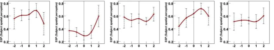
Based on the 5-point Likert scale, an analysis with standard deviations for the variations of the SSP against the semantic parameters is shown in Fig. 4. According to the linked curves of the average values of the SSP, the independent effect of a semantic parameter can be interpreted in more detail.

Fig. 4a shows an overall decline in relations between the sensation of noisiness (represented by QN, one of the parameters related to the sensation of sound intensity) and the subjective spatial perception (SSP). Namely, the more noise the audience hears, the worse their perceived spatial awareness becomes. According to Fig. 4d and 4e, the sensations of sound directivity (DO) and sound distance (CF) have similar monotonically decreasing relationships with the subjective spatial perception (SSP). It is interesting to note that a close soundscape could result in a relatively high spatial perception, while it is easy to understand that directive sounds could create a more spatial sound environment. As shown in Fig. 4b, there is also a monotonically decreasing but weaker relationship between the parameters BL and SSP.

4f. WS, STD = 0.079 4g. SIV, STD = 0.120 4h. TrD, STD = 0.043 4i. NSS, STD = 0.104 4j. SPA, STD = 0.050

Fig. 4. Independent effect of semantic parameters with the standard deviations (STD)

In contrast, Fig. 4g, 4i and 4j give the overall increasing relationships among the sensations of sound source image variations (SIV), numbers of sound sources (NSS) and subjective preferred assessment (SPA) and the subjective spatial perception (SSP), which means that more variations and numbers of sound sources may help people to increase their spatial awareness of the soundscape environments; moreover, according to Fig. 4j, people appear to prefer to like the soundscape with a little bit more spatial perception even though the feelings of boredom or liveliness for the soundscape (represented by BL, another parameter related to the overall sensation of preference) have a slight monotonically decreasing relationship with the SSP.

However, for the independent effects from the sensations of roughness (RS), sound intensity represented by WS, and transient dynamic (TrD, another parameter related to sound intensity), the situations are more complex. According to Fig. 4c and 4h, both the extreme sensations of roughness and dynamic variations of sounds may slightly benefit the subjective spatial perception (SSP), while on the contrary, either too much weak or strong sound may result in a slight aggression in relation to the spatial awareness, as shown in Fig. 4f, which means that it must be an important cue to find an optimal range of sound intensity awareness for a better subjective spatial perception. This will be discussed further in Section 3.2.2, when introducing the independent effect of Leq.

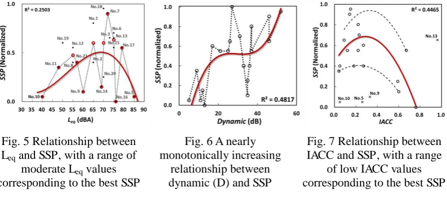
2. Effect of Leq

The acoustic parameter Leq is always a critical and positive factor for many auditory

sensations of the sound environment, including loudness, noisiness, roughness, pleasance and, of course, the spatial awareness4, 8. However, based on the results of this study, several differences are apparent: first, there is a relatively lower correlation coefficient (i.e., 0.205) between Leq and SSP, as listed in TABLE III; second, there is a range of Leq corresponding to

the best SSP due to the shape of the cubic polynomial fitting curve of Fig. 5. For example, sample 18 has the highest SSP value but not the highest Leq value. This is consistent with the

relationship between the parameter WS and SSP of Fig. 4f and contrary to the non-monotonic relationship between the parameter RS and SSP of Fig. 4f.

According to the correlation coefficients in Table 3, the sensations of noisiness (QN), roughness (RS), sound source distance (CF), weakness (WS) or variations of sound pressure levels (TrD) are highly correlated with the Leq values; normally, they also have similar

Z. Deng, J. Kang, D. Wang, A. Liu & J. Z. Kang: J. Acoust. Soc. Am. [DOI: 10.1121/1.4934272]

Journal of Acoustical Society of America, Volume 138(5), November 2015, Pages: 2860-2870 Page9 / 17

3. Effect of dynamic

According to Table 3, parameter D has the highest positive correlation coefficient (0.621) of the acoustic parameters, and its nearly monotonically increasing relationship with the SSP is shown in Fig. 6. This is similar to the sensations of sound source image variations (SIV) and numbers of sound sources (NSS) shown in Fig. 4g and 4j, respectively, but with very different from the transient dynamic sensation (TrD) shown in Fig. 4h. Namely, the sensation for dynamic changes of a real changeable soundscape environment is not exactly equal to the physical sound dynamic.

4. Effect of IACC

Another important acoustic parameter related to spatial awareness is IACC, and some models based on IACC have suggested that if the value of IACC is close to zero, this means that the sounds for two ears are uncorrelated and full of spatial perceptions. On the contrary, when the sound in the middle of two ears brings identical sound pressures on both ears, then the value of IACC is 1, which indicates no sense of spatial perceptions5. However, similar to the effect of Leq, there is a correlation coefficient of only -0.193 between IACC and the SSP,

as listed in Table 3, and excluding samples 5, 9, 10 and 13, there is also a range of low IACC values corresponding to the best SSP, as shown in Fig. 7.

Fig. 5 Relationship between Leq and SSP, with a range of

moderate Leq values

corresponding to the best SSP

Fig. 6 A nearly monotonically increasing

relationship between dynamic (D) and SSP

Fig. 7 Relationship between IACC and SSP, with a range

of low IACC values corresponding to the best SSP

3.3 Inter-relationships

1. Principal components and clusters

the perception modes of SSP.

Table 4. Results of PCA

Semantic

Parameters

Weight

Order

Total

Weight*

Component coefficients**

C1 C2 C3

QN 4 0.131 0.391 -0.076 -0.008

BL 10 0.001 -0.212 0.555 0.179

RS 7 0.106 -0.374 0.229 0.074

DO 8 0.075 -0.201 -0.362 0.452

CF 3 0.135 -0.301 -0.132 -0.552

WS 2 0.151 0.385 0.029 0.311

SIV 6 0.119 0.304 0.335 -0.391

TrD 1 0.158 0.373 0.145 0.317

NSS 5 0.122 0.325 0.222 -0.256

SPA 9 0.002 -0.216 0.550 0.194

*Normalized weight coefficients, the total summation is standardized to 1, and only the first three principal components are used to calculate the total weight of each component.

**Kaiser-Meyer-Okin measure of sampling adequacy, 0.719; cumulative 90.013%; extraction method, principal component analysis. The component coefficients are calculated by using component matrix values divided by the eigenroot of the corresponding principal component.

Table 5. HCA results and their membership parameters

Clustering

distance algorithm

Minimum rescaled

distance

Cluster and membership parameters

1 2 3

Euclidean 15 SPA BL RS DO CF SIV NSS WS TrD QN

Pearson 13 SPA BL RS DO CF SIV NSS WS TrD QN

Chebychev 23 SPA BL RS CF DO SIV NSS WS TrD QN

Minkowski 16 SPA BL RS DO CF SIV NSS WS TrD QN

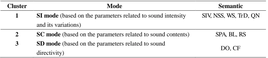
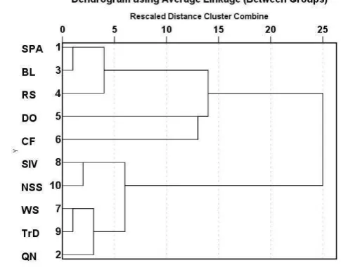
2. Perception modes of SSP

According to the minimum rescaled distances of some normal clustering distance algorithms in Table 5 and the effective component matrix values in Table 6, the optimal clusters and their corresponding SSP semantic modes with semantic parameters are shown in TABLE VI, while the Pearson clustering dendrogram is shown in Fig. 9.

Table 6. Optimal clusters and the corresponding modes of SSP with semantic parameters

Cluster Mode Semantic

1 SI mode (based on the parameters related to sound intensity

and its variations)

SIV, NSS, WS, TrD, QN

2 SC mode (based on the parameters related to sound contents) SPA, BL, RS

3 SD mode (based on the parameters related to sound

directivity) DO, CF

Z. Deng, J. Kang, D. Wang, A. Liu & J. Z. Kang: J. Acoust. Soc. Am. [DOI: 10.1121/1.4934272]

Journal of Acoustical Society of America, Volume 138(5), November 2015, Pages: 2860-2870 Page11 /

17

parameters SIV, NSS, WS, TrD, QN and Leq; C2, with a total weight of 0.236, is equivalent to

the SC mode related to sound contents and mainly dependent on the parameters SPA, BL and RS; and C3, with a total weight of 0.130, is equivalent to the SD mode related to sound directivity and mainly dependent on the parameters DO, CF and IACC. Thus, the component values of the three SSP modes can be represented by Equations (3) to (5), in which of the SSPSI, SSPSC and SSPSD are defined as the new semantic components related to the

perceptions of sound intensity and its variations (SI mode), sound contents (SC mode) and sound directivity (SD mode) respectively.

Fig. 8. Dimensions of PCA and the distributions of semantic parameters

Fig. 9. HCA dendrogram of semantic parameters, Pearson correlation method

SPA NSS TrD SIV WS CF DO RS BL QN C SSP_SI 216 . 0 325 . 0 373 . 0 304 . 0 385 . 0 301 . 0 201 . 0 374 . 0 212 . 0 391 . 0 1 ~           ₍₃₎ SPA NSS TrD SIV WS CF DO RS BL QN C SSP_SC 550 . 0 222 . 0 145 . 0 335 . 0 029 . 0 132 . 0 362 . 0 229 . 0 555 . 0 076 . 0 2 ~            (4) SPA NSS TrD SIV WS CF DO RS BL QN C SSPSI 194 . 0 256 . 0 317 . 0 391 . 0 311 . 0 552 . 0 452 . 0 074 . 0 179 . 0 008 . 0 3 ~            (5)

3.4 Linear single-value evaluation model

1. Semantic model

Fig. 10. Comparisons among SSPSI, SSPSC, SSPSD and the SSP values of Table 2

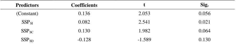
According to the algorithm of principal components analysis, the components extracted are orthogonal to each other. Thus, a linear single-value semantic regression model of the SSP can be approximated by Equation (6) with the multi-regression coefficients in Table 7.

136 . 0 128

. 0 130

. 0 082

.

0     

 SSP_SI SSP_SC SSP_SD

SSP (6)

Equation (6) has already shown that the semantic parameters of evaluation are simplified to the three components corresponding to Equation (3), (4) and (5). If the assessments of the sensations of sound intensity, sound content and sound directivity are known, then the subjective spatial perception (SSP) of a binaural-recorded soundscape sample is easy to predict.

Table 7. Regression among the new semantic components and SSP

Predictors Coefficients t Sig.

(Constant) 0.136 2.053 0.056

SSPSI 0.082 2.541 0.021

SSPSC 0.130 1.982 0.064

SSPSD -0.128 -1.589 0.130

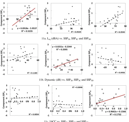
2. Acoustic model

According to linear fitting analysis, some linear regression relationships either between Leq

and SSPSI, D (dynamic) and SSPSC, or IACC and SSPSD can be found in Fig. 11.

Applying the regression formulas of Fig. 11 to Equation (6), the linear single-value semantic regression model of the SSP, represented by the parameters Leq, D (dynamic) and

Z. Deng, J. Kang, D. Wang, A. Liu & J. Z. Kang: J. Acoust. Soc. Am. [DOI: 10.1121/1.4934272]

Journal of Acoustical Society of America, Volume 138(5), November 2015, Pages: 2860-2870 Page13 /

17

11a. Leq (dBA) vs. SSPSI, SSPSC and SSPSD

11b. Dynamic (dB) vs. SSPSI, SSPSC and SSPSD

11c. IACC vs. SSPSI, SSPSC and SSPSD

Fig. 11. Linear relationships between semantic components and acoustic parameters, with the squared correlations and the solid lines suggesting the regression formula

1055 . 0 1237 . 0 0033 . 0 0075 . 0 136 . 0 ) 1566 . 0 9662 . 0 ( 128 . 0 ) 2344 . 0 0251 . 0 ( 130 . 0 ) 9537 . 5 0918 . 0 082 . 0 136 . 0 128 . 0 130 . 0 082 . 0                        IACC D L IACC D L SSP SSP SSP SSP eq eq SD SC SI (7)

3. Model test of the same set

the auditory experiment of Section 2.3, except for some minor differences with the exact values.

Fig. 12. The SSP values based on the auditory experiment, semantic and acoustic models

4. Conclusions

As discussed above, in current soundscape research efforts, many studies are focused on creating a link between acoustic parameters and psychoacoustic parameters, semantic parameters or human awareness itself and on providing an objective model to predict the corresponding subjective perception. Thus, starting from the analysis of the independent effect of 10 semantic parameters and two main acoustic parameters Leq and IACC, the

purpose of this paper was to try to reveal an evaluation model to predict the subjective spatial perception of soundscape from the above parameters.

The results of the correlation analysis and the independent effect show that the more noise (QN) an audience perceives, the less spatially aware they become, while the more closer (CF), more directional (DO), sound source image variations (SIV), numbers of sound sources (NSS) and dynamic (D) parameters the soundscape has, the better the spatial awareness would be. Then, the sensations of roughness (RS), sound intensity (WS), transient dynamic (TrD) and the values of Leq and IACC have a suitable range for a better subjective spatial perception.

Finally, a better spatial awareness seems to promote the preference (SPA and BL) slightly for an audience in a real soundscape environment.

In other words, according to the analysis of inter-relationships among all of the parameters, the awareness of the subjective spatial perception depends on the human sensations of sound intensity and its variations (SI mode), sound contents (SC mode) and sound directivity (SD mode). If assessments of the three sensations (the semantic components, SSPSI, SSPSC and

SSPSD) are given in simple a 5-point Likert scale, then the subjective spatial perception (SSP)

of a binaural-recorded soundscape sample is easy to predict by using Equation (6), or Equation (7) can be used to calculate the values of Leq, D (dynamic) and IACC with a known

awareness of sound contents.

Based on the above auditory experiments, PCA and HCA analysis, this study suggests a SSPSI-SSPSC-SSPSD semantic model and a Leq-D-IACC acoustic model to predict the

Z. Deng, J. Kang, D. Wang, A. Liu & J. Z. Kang: J. Acoust. Soc. Am. [DOI: 10.1121/1.4934272]

Journal of Acoustical Society of America, Volume 138(5), November 2015, Pages: 2860-2870 Page15 /

17

IACF), IACC (inter-aural delay time at which the IACC is observed) and ASW (apparent

source width) [24] to be examined for the spatial sensations of binaural signals in the further study. But, these two models could be important for simplifying the numbers of evaluation parameters of spatial awareness and give a quantified indicator between the sound space perception and landscapes during the soundscape planning process [25, 26].

Acknowledgments

This study is supported by the National Natural Science Foundation of China (No. 41401156), the Outstanding Training Foundation of Beijing (No. 012135407704), the “YANJING” Scholar Foundation of Beijing (No. 012155674700) and the Youth Funding Project of Humanities and Social Sciences Research Foundation from the Education Ministry of CHINA (No. 11YJCZH026).

References:

[1] R. M. Schafer, The Soundscape: Our Sonic Environment and the Tuning of the World (Alfred Knopf, New York, 1997), Introduction, pp.15-16.

[2] Y. Ando, “Orthogonal Factors Describing Primary and Spatial Sensations of the Sound Field in a Concert Hall,” Proceedings of the International Conference on Acoustics 2001 Rome, Sept. 2-7, 2001, paper 5_07.

[3] B. C. Pijanowski, A. Farina, S. H. Gage, S. L. Dumyahn and, B. L. Krause, “What is soundscape ecology? An introduction and overview of an emerging new science,” Landscape Ecology, 26, 1213–1232 (2011).

[4] B. C. Pijanowski, L. J. Villanueva-Rivera, S. L. Dumyahn, A. Farina, B. L. Krause, B. M. Napoletano, et al., “Soundscape ecology: The science of sound in the landscape,” BioScience, 61(3), 203–216 (2011).

[5] D. Y. Ma and H. Shen, Handbook of Acoustics (Science, Beijing, 2004, Chinese edition), Chap. 20, pp.574.

[6] J. Blauert, Communication Acoustics (Springer-Verlag, Berlin, 2005), Chap. 4, pp.75-103. [7] M. R. Schroeder, D. Gottlob and K. F. Siebrasse, “Comparative study of European concert halls: correlation of subjective preference with geometric and acoustic parameters,” The Journal of the Acoustical Society of America, 56, 1195-1201 (1974).

[8] H. Fastl and E. Zwicker, Psychoacoustics: Facts and Models (Springer-Verlag, Berlin, 2007), Chap. 15, pp.293-311.

[9] J. M. Potter, On the binaural modeling of spaciousness in room acoustics (Ph.D. dissertation, the Technical University of Delft, Delft, Netherlands, 1993), Introduction, pp.1-3.

[10]Y. Ando, Architectural Acoustic: Blending Sound Sources, Sound Fields, and Listeners (Springer, New York, 1998), Chap. 8, pp.120-121.

[11]Y. Ando, “A theory of primary sensations and spatial sensations measuring environmental noise,” Journal of Sound and Vibration, 241(1), 3-18 (2001).

[12]Y. Ando, “Correlation factors describing primary and spatial sensations of sound fields,” Journal of Sound and Vibration, 258(3), 405-417 (2002).

[13]B. S. Xie, X. L. Zhong, D. Rao and Z. Q. Liang, “Head-related transfer function database and its analyses,” Science in China Series G: Physics, Mechanics & Astronomy, 50(3), 267-280 (2007).

[14]C. Y. Zhang and B. S. Xie, “Platform for dynamic virtual auditory environment real-time rendering system,” Chinese Science Bulletin, 58(3), 316-327 (2013).

[15]R. Shimokura, A. Cochi, L. Tronchin and M. C. Consumi, “Calculation of IACC of Any Music Signal Convolved with Impulse Responses by Using the Interaural Cross-Correlation Function of the Sound Field and the Autocorrelation Function of the Sound Source,” Journal of South China University of Technology (Natural Science Edition), 35(Supplement), 88-91 (2007).

[16]J. Liu, J. Kang, T. Luo, H. Behm and T. Coppack, “Spatiotemporal variability of soundscapes in a multiple functional urban area,” Landscape and Urban Planning, 115, 1-9 (2013).

Z. Deng, J. Kang, D. Wang, A. Liu & J. Z. Kang: J. Acoust. Soc. Am. [DOI: 10.1121/1.4934272]

Journal of Acoustical Society of America, Volume 138(5), November 2015, Pages: 2860-2870 Page17 /

17

individually,” The Journal of the Acoustical Society of America, 134(1), 803-812 (2013). [18]J. Hong and J. Y. Jeon, “Designing sound and visual components for enhancement of

urban soundscapes,” The Journal of the Acoustical Society of America, 134(3), 2026-2036 (2013).

[19]S. Dance and P. Wash, “MP3 listening levels on London Underground for music and speech,” Applied Acoustics, 74(6), 850-855 (2013).

[20]W. Yang and J. Kang, “Acoustic comfort evaluation in urban open public spaces,” Applied Acoustics, 66, 211-229 (2005).

[21]D. W. Wang, Z. Y. Deng, X. X. Li and A. L. Liu, “Temporal features extraction for the binaural soundscape samples,” Proceedings of INTERNOISE 2014 (Melbourne, Australia, November 16-19, 2014), paper No.901.

[22]Z. Y. Deng, D. W. Wang, A. L. Liu, H. K. Chen and J. Zhangn, “Semantic Assessment for the Soundscape of Chinese Ethnic Historical Areas,” Proceedings of INTERNOISE 2013 (Innsbruck, Austria, September 15-18, 2013), paper No.0123, pp.268.

[23]J. Kang and M. Zhang, “Semantic differential analysis of the soundscape in urban open public spaces,” Building and Environment, 45(1), 150-157 (2010).

[24]Y. Ando, Auditory and Visual Sensations (Springer, New York, 2009), Chap. 7, pp.125-136.

[25]X. Ren and J. Kang, "Effects of visual landscape factors of ecological waterscape on acoustic comfort," Applied Acoustics, 96, 171-179 (2015).