S o n g X i C h e n
A th e s is s u b m i t t e d fo r t h e d e g r e e o f
D o c t o r o f P h ilo s o p h y
o f
T h e A u s t r a l i a n N a t i o n a l U n i v e r s i t y
C e n t r e fo r M a t h e m a t i c s a n d I t s A p p lic a tio n s
A c k n o w l e d g e m e n t s
I would like to express my deepest g r a t i t u d e to m y super vi sor , Professor P e t e r Hall for his excellent supervision and insight. He i n t r o d u c e d me to t h e s ubj ect t r e a t e d in this thesis, and as a whole op ened my eyes to m o d e r n t e chniques of stat istics. His e nc o ur a g e m en t s and cons tr uct i ve criticism were i m p o r t a n t stimuli for this thesis. I would like to t h a n k Drs. A n d r e w Wood a nd Dar yl Dayley of ANU , a n d Professor Ar t Owen of Stanf or d University for beneficial discussions and e nc o ur a g e m en t s . A special t h a n k s goes to my fellow s t u d e n t R o b e r t Mur is on for his friendship an d tennis games which I enjoyed so mu ch d ur i n g my two years stay in C a n b e r r a . I also would like to t h a n k th e people a t t he Ce n t r e for M a t h e m a t i c s an d Its Appli cat ions and in b o t h Statistics D e p a r t m e n t s of ANU for th ei r s u p p o r t and assistance, which make my ti me at ANU t he m o s t enjoyable.
I am great ly i nd e bt ed to my wife, Ling, for her c ont i nu ed help, e n c o u r a g e m e n t and love over t he last two years. It is never easy to be a P h . D s t u d e n t ’s wife. I am also i n d e b t ed to bo th families of us in C h in a , for their endless love a nd mor al s u p p o r t .
T h e following p a pe rs have been s u b m i t t e d for pub li c at i on from t he work c ont ained in this thesis:
C H E N , S.X. an d HALL, P. (1991). S m oo th e d e mpir ica l likelihood confidence i n t e r vals for quantiles. A n n . S ta t is t, to a p pe a r .
C H E N , S.X. (1991). On the accur acy of empir ical likelihood confidence regions for l inear regression model. A n n . Inst. Stat i st . M a t h , to a p p e a r .
C H E N , S.X. (1992a). Empi ri ca l likelihood confidence intervals for linear regression coefficients. S u b m i t t e d to Jour na l o f M ul t iv ar ia te A n a l y s i s., May, 1992.
m e t h o d of inference with s a mpl ing p r oper ti es similar to those of th e b o o t s t r a p . However, in s te a d of assigning equal pr obabilities n -1 to all d a t a values, empirical likelihood places a r b i t r a r y pr obabilities on th e d a t a poin ts, say p, on t he i ’th d a t a value. T h e weights p, are chosen by profiling a m u l t i n o m i a l likelihood s u p p o r t e d on t he s ampl e, a nd empirical likelihood confidence regions are c o n s t r u c t e d by con t o u r i n g this m u l t in om i al likelihood. An a t t r a c t i v e f eat ur e of empir ical likelihood is t h a t it p rod u ce s confidence regions whose s hapes a nd o r ie nt a ti o ns are d e t e rm in e d ent ir ely by the d a t a , and which have coverage a cc ur acy at least c o m p a r a b l e with th o se of b o o t s t r a p confidence regions. In C h a p t e r 1 of this thesis we review t he con cepts of empir ical likelihood and its devel opment s. We also outl ine th e noti ons of E d g e w o r t h expans ion which is an i m p o r t a n t tool of s t u d y i n g t he coverage pr oper ti es of e mp ir ica l likelihood confidence regions.
In C h a p t e r 3 we consider the second n o n - s t a n d a r d case, which is to c on s t r u c t e m pi r i c al likelihood confidence region for t he regression coefficient vector ß of a li near regression model Y, = X{ß + 6, , 1 < i < n. Due to t he presence of the fixed design p oi nt s, t he observed r a n d o m variables are i n d e p e n d e n t b u t n ot identically d i s t r i b u t e d . So it is not the s t a n d a r d i n d e p e n d e n t a nd identically d i s t r i b u t e d r a n do m s a mp l e case any more. E m p ir ic a l likelihood m e t h o d s were p r op os e d by Owen (1991) for c on s tr u c t i n g confidence regions for ß in th e mo d el (3.1.1). He derived a n o n p a r a m e t r i c version of W i l k s ’ t h e o r e m , e ns u ri ng t h a t empir ical likelihood con fidence regions for ß have correct a s y m p t o t i c coverages. We show t h a t coverage er ro rs of t he empir ical likelihood confidence regions for ß are of or der to- 1. B a r t l e t t cor rect ions ma y be employed to r educe the coverage er ror s to 0 ( n ~ 2). For pr act ical i m p l e m e n t a t i o n of B a r t l e t t correct ion, we also give an empir ical B a r t l e t t correction.
It is not eno ug h to j us t c o n s t r u c t confidence regions for ß of a linear regression mode l. In pr act ice, stat i st ic ian s are often confronted with pr o bl em s of c o ns t r u ct i n g confidence intervals for a p a r t i c u l a r regression coefficient or for cer tain linear c o m b i na t i o ns of ß. In C h a p t e r 4 we add re s s the above p r o bl em u n d e r t he simple linear regression model: y,- = a0 + b0Xi -f et-, 1 < i < n. N o n p a r a m e t r i c versions of W i l k s ’ t h e o r e m are proved for empirical likelihood of th e slope p a r a m e t e r b0 a nd me a n p a r a m e t e r y 0 = a 0 + b0 x 0 for any Used x 0, which enabl e us to c o n s t r u c t empir ical likelihood confidence intervals for t hese p a r a m e t e r s . We also show t h a t coverage errors of these confidence intervals are of or der n -1 an d can be reduce d to or der n ~ 2 by B a r t l e t t correction.
A ck n o w led g em en ts 2
R e la te d p u b lic a tio n s 3
A b s t r a c t 4
C H A P T E R O N E
C O N C E P T S OF E M P I R I C A L L I K E L I H O O D A N D E D G E W O R T H E X P A N S I O N S
1.1 I n tr o d u c t io n 1
1.2 C o n c e p ts of E m p irical Likelihood 3
1.3 E d g e w o rth E x p an sio n s 9
1.3.1 E d g ew o rth E x p an sio n s for i.i.d Case 10
1.3.2 E d g ew o rth E x p an sio n s for a non-i.i.d Case 12 1.3.2 T ra n s fo rm a tio n of E d g ew o rth E x p an sio n 13
1.4 M o tiv a tio n and S u m m a ry of Thesis 16
C H A P T E R T W O
E M P I R I C A L L I K E L I H O O D C O N F I D E N C E I N T E R V A L S F O R Q U A N T I L E S
2.1 I n tr o d u c tio n 19
2.2 U n s m o o th e d E m p irica l Likelihood Confidence Interv als for Q u an tiles 20 2.3 S m o o th e d E m p irical Likelihood Confidence Intervals for Q u an tiles 23
2.3.1 N o tatio n and L em m as 24
2.3.2 W ilk s ’ T h eo re m and Coverage A ccuracy 28
2.3.3 B a r t le tt C orrection 30
2.4 S im u latio n S tu d y 33
2.5 P roofs 48
2.5.1 P ro o f of L em m a 2.3.2 48
2.5.2 P r o o f of T h eo re m 2.3.3 49
C H A P T E R T H R E E
O N T H E C O V E R A G E O F E M P I R I C A L L I K E L I H O O D C O N F I D E N C E R E G I O N S F O R L I N E A R R E G R E S S I O N M O D E L
3.1 I n tr o d u c tio n 66
3.2 W ilk s ’ T h e o re m an d Coverage A ccuracy 67
3.3 B a r t le tt C o rrectio n 74
3.4 S im u latio n S tu d y 77
3.5 P roofs 82
3.5.1 P r o o f of L e m m a 3.2.1 82
3.5.2 P r o o f of T h eo re m 3.3.1 85
3.5.3 P r o o f of T h eo re m 3.3.2 85
A p p e n d ix 3 C a lcu latio n of c u m u la n t of n? R 92
C H A P T E R F O U R
E M P I R I C A L L I K E L I H O O D C O N F I D E N C E I N T E R V A L S F O R L I N E A R R E G R E S S I O N C O E F F I C I E N T S
4.1 In tr o d u c tio n 97
4.2 P relim in a ries 98
4.3 E m p iric a l Likelihood Confidence Interval for Slope P a r a m e te r 100
4.3.1 W ilk s ’ T h eo re m 101
4.3.2 Coverage A ccuracy and B a r tle tt C o rrectio n 104
4.3 E m p irica l Likelihood Confidence Interval for M eans 108
4.4.1 W ilk s ’ T h e o re m 108
4.4.2 C overage A ccuracy and B a r t le tt C o rrectio n 112
4.5 S im u latio n S tu d y 114
4.6 P roofs 120
4.6.1 P r o o f of T h eo re m 4.3.2 120
4.6.2 P r o o f of T h eo re m 4.3.3 121
C H A P T E R F I V E
C O M P A R I N G E M P I R I C A L L I K E L I H O O D A N D B O O T S T R A P H Y P O T H E S I S T E S T S
5.1 I n t r o d u c t i o n 139
5.2 E m p i r i c a l Likelihood and B o o t s t r a p Hypothes is Tests 140
5.2.1 Em pi ri ca l Likelihood Tests 141
5.2.2 B o o t s t r a p Test 142
5.3 P owe r E x p a ns i o ns 143
5.3.1 Power of (J)ec 144
5.3.2 Power of <f>b 147
5.4 P ower C o m pa r i s on s 150
5.4.1 T h e Univariate Case 151
5.4.2 T h e Bivariate Case 151
5.5 S imu lat i on S t u d y 154
5.6 Proofs 158
A p p e n d i x 5 Cal culat ions of c u m u l a n t s 159
A p p e n d i x 5.1 Cal culat ion of C u m u l a n t s of n? R (t) 159 A p p e n d i x 5.2 Cal culat ion of C u m u l a n t s of n? S ( r ) 168
w & n © £ ®o
The tao
that can be said is not the everlasting Tao.
I f a name can be named, it is not the everlasting Name.
That which has no name is the origin o f heaven and earth
That which has a name is the Mother o f all things
1.1 I n t r o d u c t i o n
T h e coming of the c o m p u t e r age in the last a few decades has deeply changed t h e s hapes and t h e ways of t h i nk in g of the centuries old displine called Statistics. T h e m os t n o t a b l e event was t he bi rt h of th e b o o t s t r a p m e t h o d in 1979 by Efron (1979) a nd t he following works done in 1980s, leading t he b o o t s t r a p be com ing a m a t u r e general stat i st ic al p r o c e d u r e with wide rang e of appl i cat i ons . Hall (1992) gave a full d es cr ipt ion of the d ev el opment and t he or y of t h e b o o t s t r a p . An i m p o r t a n t f eat ur e of t h e b o o t s t r a p is t he idea of “r e s a m p l i n g ” . In t he p r e - b o o t s t r a p era, s tat i st ic ian s d e p e n d e d heavily on t he C en t r a l Limit T h e o r e m , which gives a n o r m a l a p p r o x i m a t i o n to a stat istic of interest. However, this a p p r o x i m a t i o n only takes into acc ou nt t he first two m o m e n t s w i t h o u t t a ki ng care of skewness a nd kur tosis of t he stat istic, causing t h a t t he accur acy of t he a p p r o x i m a t i o n is only of first order. By g e ne ra t in g a large n u m b e r of r esampl es o ut of t he original sa mpl e in a c o m p u t e r , t he b o o t s t r a p implicitly corrects skewness an d kur tosis d ur i n g th e r e s am pl i ng p r o cedure. Thi s leads to a mor e a c c u ra te a p p r o x i m a t i o n to t he d is t r i b u t i o n of the statistic.
for survival probabil it y. Tho se a u t h o r s show t h a t t he confidence intervals have the desired p r o p e r t y of res pect i ng r ange, which is not generally held by n o r m a l a p p r o x i m a t i o n b as ed m e t h o d s . However, Owen was th e first to s yst ema ti ca ll y d e m o n s t r a t e t h a t t h e ide a has very wide r ange of appl icat ions.
It has been shown t h a t n o n p a r a m e t r i c versions of W i l k s ’ t h e or em and B a r t l e t t correct ion hold t r u e for empir ical likelihood in a wide r an ge of s i tu at io ns , akin to t he u s u al p a r a m e t r i c likelihood. However, c o m p a r e d with p a r a m e t r i c likelihood, emp ir ica l likelihood is r o b u s t since it is c o n s tr u ct e d in a way which does n ot as sume t he form of the d i s t r i b u t i o n . C o m p a r e d with t he b o o t s t r a p , e mpir ica l likelihood has several a d v an t a ge s . Hall and La Scala (1990) have identified t h e following a t t r i b u t e s :
(1) E mp i r i c a l likelihood enabl e the s ha pe and o r ie nt a ti o n of a confidence region to be d e t e r m i n e d “a u t o m a t i c a l l y ” by t he s ampl e, wher eas c o ns t r u ct i o n of a m u l t ivar iat e b o o t s t r a p confidence region requires a decision on how t he region should be s h a p e d a nd o rient ed since the b o o t s t r a p itself c a n n o t provide an answer to any of these. It can be very h a r d to decide w h e t h e r to use an elliptical or r e c t a n g u l a r confidence region.
(2) E mp i r i c a l likelihood confidence regions are B a r t l e t t cor rect ionabl e, m e a n i n g t h a t a simple a d j u s t m e n t for scale reduces t h e or der of m a g n i t u d e of coverage error from n ~ 1 to n~ 2, wh er e n denotes sampl e size. (See DiCiccio, Hall and R o m a n o 1991.) T h e b o o t s t r a p confidence region can a t t a i n t he s a me or de r of coverage accuracy. However, t h e b o o t s t r a p achieves this at expensive of e n o r m o u s c o m p u t e r hours.
r a t i o of me a n s .
(4) E m p i r i c a l likelihood confidence regions are r ange r es pect ing, as was noti ced by T h o m a s a nd G r u nk em ei e r (1975). For exampl e, th e empi ri ca l likelihood confi dence region for a correlation coefficient always lies withi n interval ( — 1,1). However, this p r o p e r t y is n ot necessarily preserved by a b o o t s t r a p confidence region; consider for e x a m p l e confidence regions c on s tr u ct e d using th e per centil e- t m e t h o d .
T h e basic concepts of empir ical likelihood are given in Section 1.2, t o g e t h e r with s ome f u n d a m e n t a l formulae and expans ions used by e mpir ica l likelihood. In Section 3.1 we display some existing results of E dg e w o r t h e x pa ns io n, which will be t h e basic tool used in this thesis to s t ud y coverage acc ur acy a nd B a r t l e t t corr ect ion of e m pi ri ca l likelihood confidence region. We provide an outl ines of this thesis in Section 1.4
1 . 2 C o n c e p t s o f E m p i r i c a l l i k e l i h o o d
In this section we describe the basic concept of e mpir ica l likelihood. S u p po s e X i, • • •, X n are p- dimens ional i n d e p e n d e n t and identical d i s t r i b u t e d (i.i.d.) r a n d o m vectors from u n k n ow n d i s t ri b ut io n F. Let 0 = 0 ( E ) de no t e some c ha ra c t e r i s t i c of F, such as m e a n , variance etc, for which we want to c o n s t r u c t a confidence region (or int er val) . Wr it e P i , V i > ’' ' -> P n for n onnegat i ve n u m b e r s a d d i n g to unit y, and
6(p) for t he value of 6 when the di st ri b ut io n f unction F is replaced by
wher e I is t h e ind i ca to r functi on. We can view Fp ( x) as weighted em pi ri ca l d i s t r i b u n
Ep ( z ) = P i ! { x i < x ), i = 1
tion f unct i on . For i ns ta nce if 6 denot e the p op u l a t i o n m e a n , t h a t is 9 = f x d F ( x ) ,
n
If we i m p os e only one c o ns t ra i nt , Y P i = 1, while m a xi mi z in g n " = 1 P», we get
Pi = n ~ 1 for i = 1 which gives us th e b o o t s t r a p e s t i m a t e 0 = 0 ( F ) f ° r where
n
F( x ) = ^_1 /(*,- < x)
» = l
is t he emp ir ica l d i s t r i b u t i o n f unction. T h u s , we have
L( 0) = n ~ n .
Now t he emp ir ica l log-likelihood ratio , eval uated at 0 = 9X, is defined as
1(6, ) = - 2 log{ 1 ( 9 , ) / ! ( « ) }
n
= - 2 min 5 Z log ( n P*)* (1.2.1)
0 ( P ) = 0 i . I Z P . = 1 x
It is well-known t h a t u n d e r certain regular ity c ondi tions , th e us ual p a r a m e t ric log-likelihood r at i o has the following pr oper ti es : (1) it converges in d i s t ri b ut io n to Xp5 t he chi-square d i st r i b u ti o n with p degrees of f reedom, as s a mpl e size n a p proaches to infinity; this is W i l k s ’ t he ore m (Wilks 1938); (2) it is B a r t l e t t cor rect able ( B a r t l e t t 1937, Lawley 1956). W i l k s ’ t he o re m enabl e us to c o n s t r u c t confidence r e gions by looking up t h e Xp tables, and B a r t l e t t correct ion can be used to impr ove th e coverage acc u ra cy of the confidence region by simple a d j u s t m e n t to t he me an of the log-likelihood r at i o statistic.
r e g ul a ri ty conditions:
(i) E = C o v ( Ti) is positive definite ma t ri x; (ii) £ | | X 1||a < oo;
(iii) for every positive b, the char acter ist ic f uncti on g of X \ satisfies ^ ^ 2) C r a m e r ’s condi tion sup \g(t)\ < 1,
ll*ll>*
whe re 5 = 5 for t h e me a n case and 5 = 15 for th e s m o o t h f uncti on of m e a n s case. T h e reg ul ar it y co ndi tions as sumed for t he regression case are described in C h a p t e r 3.
In t he rest of this section we give some basic f or mul ae and a l g o ri t hm s for the case of 0 = /I = f x d F ( x ) , which has been used by pr evious a u t h o r s an d will be referenced r e p e a te dl y in this thesis for c on s tr u c t i n g emp ir ica l likelihood confidence regions in o t h e r situa ti on s.
Ac cor ding to (1.2.1), the empirical log-likelihood r at i o for 6 = fi, e val uate d at A* = Mi, is
n
^(Mi) = - 2 min 5 1 l og( n pi). (1.2.3)
zJ
P t x . = ^ 1 >X/
P i =1 i=1Using the L ag ra ng e mu ltip lier m e t h o d to solve t he above op t i ma l i z a t i o n pr oblem (1.2.3), it t u r n s o u t t h a t the o p ti ma l p . ’s have th e following form:
1 1
n 1 -f t T (X i — fi) ’ 1 < i < n,
wher e t = (C , • • • , t p )T satisfies
(1.2.4)
X j - f i 1 + t T ( X i - p )
S u b s t i t u t i n g (1.2.4) int o (1.2.1) we o bt a i n
n
i ( ß ) - 2 5Z l o g { l + t T ( X i - jt)}.
(1.2.5)
:= 1
i= 1 wher e A = (Ax,• • • , Ap )T = £ 2 J satisfies
■ £
Zi
1 + AT 2j
= 0. (1.2.8)
Since a na l yt ic solution for A in (1.2.8) is not a t t a i n a b l e , we have to r esor t to e x p a n sion. Before doing t h a t , let us first define
a j ' -jk = E ( z l 1 • • • z j k ) ,
" (1.2.9)
A *1'"** = n - 1 ^ z \ x • • • z \ k — a j l '"j k .
i= 1
We see a jl "ik is a Ar’th or der m u l t iv a ri at e m o m e n t of Z, a nd is a A:’th or der cent ral m u l t i v a r i a t e me a n of Z j ’s.
Owen (1990) set up an one- te rm Taylor expan sion for l ( n) :
i {^i ) — n A j A j + O p(n 1^2). (1.2.10)
T h r o u g h o u t this thesis we use t he s u m m a t i o n convent ion t h a t t e r m s with r e p ea t ed indices are to be s u m m e d over. From (1.2.10) we are able to prove the following n o n p a r a m e t r i c version of W i l k s ’ t h e o re m by a s s um i ng condi tion (i) of (1.2.2) ,
^ O ) Xp> as n —> 00, (1.2.11)
since y/ n A = ( A 1, • • •, Ap ) converges to A ( 0 , / p ) in d i s t r i b u t i o n by t he C en t r a l Limit T h e o r e m , where I p is t he p- dimens ional ide nt it y m a t r i x . An a-level confidence region for fi can be c o n s tr u ct e d in the following way. F i r s t find from th e Xp tables the value ca such t h a t
to be devel oped. After Taylor e xpan si on, as has been shown by DiCiccio, Hall and R o m a n o (1988), A has the following expansion:
Xj = A j - A jk A k + a jkl A* A 1 + A jl A kl A k + A jkl A* A 1
- a klm A jm A k A 1 - 2 a jkm A ,m A k A 1 + 2 a jkn a tmn A k A 1 A m (1.2.12) - a jk,m A fc A 1 A 1 + 0 p{ n ~ 2).
S u b s t i t u t i n g ( 1.2 . 12) into (1.2.13), we o bt a in
7 i - ^ ( / i ) = A j A j - A j k A j A k + § a j k l A j A k A l + A j 1 A k 1 A j A K
+ § A j k l A j A k A l - 2 a j k m A l m A j A k A l + a j k n a , m n A j A k A l A m
- ^ a j k l m A j A k A ' A m + Op ( n - 5/ 2). (1.2.13)
A signed root d eco mp os it i on for £(fi) can be derived from (1.2.13), t h a t is,
l ( ß ) = ( n , / 2 R T ) ( n 1/2R ) + O p( n - 3/ 2), (1.2.14)
where R = R i + R 2 + R3 is a p-dimensional vector a nd Ri = O p ( n ^ 2) for l = 1, 2, 3. C o m p a r i n g t e r m s in (1.2.13) with those in (1.2.14) yields,
R \ = a>,
R i = - ' - A i k A k + ± a i k m A kA m and
ß j _ I ^ 4j m m k m _____ — a J k m A * m A k A1
3 8 3 12
- a ~ - ’ A j m A k A l + 1 a j k n a 1 m n A m A k A 1 — ^ a j kl m A m A k A1,
where R j{ is t he j ’t h c o m p o n e n t of R t . Notice t h a t t he re exists a s m o o t h f uncti on h 0 such t h a t R = h 0( U0), where U0 = ( A 1, • • •, Ap , A 11, • • • App, A 111, • • •, APPP)T is a me a n of i.i.d. r a n d o m vectors. So, R is a s m o o t h f uncti on of i.i.d. me a ns . T h u s , after cal cu la ti ng joint c u m u l a n t s of R, a nd using th e valid E d g e w o r t h expan si on developed by B h a t t a c h a r y a and Ghosh (1978) for this case, it can be shown t h a t u n d e r co ndi tio n ( 1.2 .2 ) for any x > 0 ,
T hi s implies t h a t
P(/x € I a ) = a - ß 0 ca gp(ca ) n 1 + 0 ( n 2),
which m e a n s t h a t t he coverage acc ur acy of th e empir ical likelihood confidence region I Q is of or d er n ~ 1. We know t h a t in the p a r a m e t r i c case, p a r t of th e coverage er ror of a confidence region c on s tr u c t e d by the log-likelihood r ati o m e t h o d is due to th e m e a n of the log-likelihood rati o not being equal to p, which is t he m e a n of t h e Xp d i s t r i b u t i o n . B a r t l e t t correction can be used to impr ove th e coverage acc ur acy by r e a d j u s t i n g t h e me a n of t he log-likelihood ratio. For t he case of s m o o t h f uncti on of m e a n s , DiCiccio, Hall a nd R o m a n o (1991) showed t h a t t he e mpir ica l likelihood confidence region is B a r t l e t t cor rect able, which implies t h a t a simple a d j u s t m e n t for th e me a n can reduce the coverage error from or der n ~ 1 to or d er n ~2. From e xp ans io n (1.2.13) the above a u t h o r s showed t h a t
E { t ( ß ) } = p ( l + ß o n - 1) + 0 ( n ~ 2),
where ß 0 is t he B a r t l e t t f actor given by (1.2.15). It can be shown t h a t
P { i { p ) < cQ ( l + Co«- 1 )} = & + 0 ( n ~ 2), (1.2.16)
where Co is ei ther ß 0 or a r o o t- n consistent e s t i m a t e of ß 0. From (1.2.16), we can correct t h e confidence region I a by defining
J a = { M U M < Ca ( l + Co «" 1)},
ical likelihood confidence regions. So it is wor thwhile to devote this section on it. In this section we display some existing results on E dg e w o r t h e xp ans ions , for e xampl e as des cr ibed in B h a t t a c h a r y a a nd Ra o (1976) a nd B h a t t a c h a r y a a nd Gh os h (1978). T h es e result s will be used r e p e a t e d l y in this thesis to derive a s y m p t o t i c expans ions of d i s t r i b u t i o n s of t he empir ical log-likelihood r ati o stat istics in various sit ua ti ons . In p a r t i c u l a r , we are int er es ted in E dg e w o r t h e xpans ions for d is t r i b u t i o n s of s m oo t h f uncti on of a m e a n , where t h e me a n could be an average of ei ther i.i.d. r a n d o m vectors or i n d e p e n d e n t b u t n ot identically d i s t r i b u t e d r a n d o m vectors. Before doing this we give some n ot a t i o n .
Let F be t h e d is tr i bu ti on f uncti on of a r a n d o m vector X £ R fc with c h a r a c t e r istic f uncti on p. If f ||x||ad F ( x ) < oo, we ma y have th e following Tayl or ex pans ion
log{v?(t)} = X« (*t)v /v! -F o(||t||*), as t -> 0, (1.3.1) M< *
where t = ( G, • • • ,£ * ) and v = (rq, •••,u*; ) is a n on ne ga t iv e vector of integers with o p e ra t i on s |v| = X) t v, and (i t ) v = ( i t i ) Vl • • • ( i t k )Vk. T h e coefficient Xv a p p e a r i n g in (1.3.1) is called t he u ’th c u m u l a n t of F . For a given set of Xv •> we define p olynomial s
X/(*) = H M = i V '
for any positive integer /, wher e z v = z ”1 • • • z vkk for z — (-2q , • • • , z k) £ R *\ M o r e over, we define p olynomial s P s (z : {Xv}) by t he following f or mal e qu at i on in a real variable u,
OO OO 1 OO , v
1 + Ps ( z : {Xt,})u* = 1 + 77 { XZ 7*+;2 - u } l .
5 = 1 / = 1 Z! * = 1 v (s + 2 )!'
Let V = C o v ( X ) , <f>o,v a nd $ 0,v be the n o r m a l densit y a nd d is t r i b u t i o n functi ons in R fc with zero me a n and covariance m a t r i x V respectively, an d p u t
„ dv1 d Vk
D 4>o,v — (po,v (x) •• * 77777 777“ <t>o,v (x
F u r t h e r m o r e , let P r ( — $ 0y * {Xv }) be t h e finite signed m e a s u r e on TLk with density Pr(-(f>0>v :
{x„})-1 . 3 . {x„})-1 E d g e w o r t h E x p a n s i o n s f or i . i. d . C a s e
S u p po s e X i , - - * , X n are i.i.d r a n d o m vectors d r a w n from d is t r i b u t i o n F with me a n p , covariance m a t r i x V a nd char act er ist i c functi on <p. Let
n
W = n - 1/2 £ ( X , - m). * = 1
T h e n we have t h e following t he o re m due to Esseen (1945) a nd B h a t t a c h a r y a (1968):
T h e o r e m 1 . 3 . 1 A s s u m e that F has finite s ’th absolute m o m e n t f o r s ome integer s > 3, and satisfies the C r a m e r ’s condition sup|| t ||>6 |y?(t)| < 1 f or any positive b.
Then,
3 - 2
sup I P(W€ B ) - £ n - r/2 P r ( - < f o,v : { x , } ) ( B ) | = o ( r r < ' - 2)/2), (1.3.2)
B6B r = o
where B is any class o f Borel sets satisfying
sup I <f>0tV ( v) d v = 0 ( e ) , e I 0, (1.3.3) B t B J ( d B ) '
and d B and (d B ) e are the boundary o f B and e-neighborhood o f d B respectively.
Let f i, • • •, f m be real-valued Borel m e a s u r a b l e f uncti ons on R fc , h be a s m o ot h real-valued functi on on R m , and Q, = ( f i (X, ), • • • , f m (X,-)) for 1 < i < n. Cons ider a st at i st ic
T„ = n ' l 2 { h ( Q ) - h ( n q)},
where Q = n ~ l 52 j Qi and p q = E ( Q i ) . Clearly T n is a s m o o t h functi on of Q. P u t
Co ns id er t he following Taylor expans ion of Tn a r o u n d fiq,
5 — 1
< = n1/2E E (fci
~k = 1 * 'i
wher e Q k a nd [ilqk are the z*fc ’th c om p o n e n t s of Q and /i? respectively. Using t h e d e l ta m e t h o d we m a y exp ec t t h a t t he E d g e w o r t h e xpans ion of t h e d is t r i b u t i o n of
Tn a nd Tn generally disagree only in t e rm s of or d er n~ (-s~ 2^ 2 or smaller, i.e
P( T„ < x ) = P( T„ < x) + 0( n - < * - 2)/2),
since Tn — Tn = op ( n~ 2^ 2). Now, t he c u m u l a n t s of Tn are muc h easier cal culated t h a n tho se of Tn , since Tn is a m ul t iv a ri at e p ol ynom ia l in Q — /z9. If Q\ has sufficiently m a n y m o m e n t s t h e n , as shown by J a m e s and M a y n e (1962), t h e j ’th
/
c u m u l a n t k j n of Tn is given by
kj,n ^ kj,n + °( n
~^2),
~ /
wher e kj n is an “a p p r o x i m a t e c u m u l a n t ” of Tn , havi ng t he form
L _ f S ’=12 n " /2 bji if j
4
- 2;\ <T2, + 1 2 1 : 1 n - ‘' * b2iif 2, an d bj i ’s d ep e n d only on the m o m e n t s of Z x an d on derivatives of h at /i9. T h e c har act er i st i c functi on of Tn (or Tn ) can be a p p r o x i m a t e d by
T n (t) = exp{«t k 1>n + ^ - ( k 2>n - er]) + ~ f " h. n } e x p ( - o r V / 2 ) . (1.3.4)
2! v 7!
j = 3
After e x p a n d i n g t he first e x po ne nt i a l factor in (1.3.4), we o b ta i n i - 2
T n(t) = e x p ( —<72^2/ 2 ) { l + n ~ r/2 7rr ( ^ ) l + o ( n ~ {s~ 2)/2),
— OO
wher e
« — 2
1>,,n = {1 + n ~ r/2 wr ( - d / d v ) } <f>a*(v).
r = 1
B h a t t a c h a r y a a n d Gh osh (1978) proved t h a t is a valid E d g e w o r t h ex pans ion of t he d i s t r i b u t i o n of T n . P a r t of t he ir results are s t a t e d in th e following t he or em:
T h e o r e m 1 . 3 . 2 A s s u m e that (i) h has cont inous derivatives up to order s > 3 in a neighborhood o f p q; (ii) E \ Q i \ s is finite; (in) C r a m e r ’s condition holds f or Q \ , that is l i m s u p ^ i ^ . ^ | E { e x p ( i < t , Q i > ) } | < 1, where < > denotes the Euclidean i n ne r product on R * . Then,
sup | P ( T n € B ) - f xfS}n( v ) d vI = o ( n _ ( , _ 2 ) / 2 )
b&b J b
u ni f or ml y holds over the class o f B satisfying (1.3.3).
1 . 3 . 2 E d g e w o r t h E x p a n s i o n for a n o n - i . i . d c a s e
In this subsecti on we display result for s e t t in g up E dg e w o r t h expan sion for a non-i.i.d case. T h e case we consider is t h a t t he s a mp l e X i , • • ■ , X n are i n d e p e n d en t b u t n ot necessarily identically d is t r i b u t e d r a n d o m vectors in R fc. Thi s is j us t t h e s i t u a ti on of a linear regression mod el , wher e t h e presence of t h e fixed design po in ts makes t h e r es pons e r a n d o m variables are i n d e p e n d e n t b u t n ot identically d i s t r i b u t e d .
(i) V k tn u n if o rm ly bounded away from zero; (ii) the average s-th absolute n
m o m e n t s n ~ l ^ E(|| X, ||)* are bounded away from infinity f or s > 3;
« = l
(Hi) f o r each positive €, lim n -1 ^ / ||Xi||* = 0; (iv) the (1.3.5)
n_"°°
i=i 'V;ll
><«1/2
characteristic f u n c t i o n s gn o f X n satisfies C r a m e r ’s condition lim sup s up \gn (i)| < 1, for every positive b.
n — oo || <|| > 6 Then
s —2
s up \P(S„ € B ) - E n - r / 2 P r ( - $ 0iv : { x if„ } ) ( B ) | = r = o
over the class o f B satisfying (1.3.3).
1 . 3 . 3 T r a n s f o r m a t i o n o f E d g e w o r t h E x p a n s i o n
We show in T h e o r e m 1.3.2 t h a t t he E dg e w o r t h expan si on for t he d i s t ri b ut io n of an i.i.d. m e a n can be t r a n s f o r m e d by a s m o o t h functi on to yield a n o t h e r valid E d g e w o r t h e xp an si on. We also show t h a t this e xpans ion ma y be cal culated from th e c u m u l a n t s o b t a i n e d by using the del t a m e t h o d , i.e th e c u m u l a n t s formally cal c ul ated from a Tayl or expans ion o m i t t i n g t e rm s of higher order. S kovgaar d (1981) generalized the above result of B h a t t a c h a r y a and Ghosh (1978). He d e m o n s t r a t e d , using t he d e l ta m e t h o d , t h a t any (not j u s t for i.i.d. m e a n ) valid E dg e w o r t h ex pan si on m a y be t r a n s f o r m e d by a sequence (not j u st a single s m o o t h f uncti on) of sufficiently s m o o t h functi ons to get a n o t h e r valid E d g e w o r t h expans ion.
5 - 2
^ >
Pr{^0,/fc •
{Xo,n}) (u))
r — o
ßs ,n = [sup{ ||Xw ,n ||1/(H_2) | 3 < |v| < 5 }] ' 2 = o ( l ) ,
a n d {xv,n •> 3 < \v\ < s } are t he c u m u l a n t s of Un . Clearly we have x«,n = 0 for |u| = 1, since E ( U n ) = 0. W h e n Un is a nor mal ized sum of i n d e p e n d e n t a nd identical d i s t r i b u t e d r a n d o m vectors, we have ß s n = 0 ( n ~ ^ s~ 2^ 2) as Xv,n = 0 ( n ~ ^ v^~2^ 2).
Let {h n } be a sequence of functi ons m a p p i n g into R m for m < k. For each n, h n is p- ti mes differentiable at zero (p > 2) and satisfying h n (0) = 0 a nd the J a c o b i a n m a t r i x of h n at zero, say D h n (0), is of r a nk m . P u t
B n = { D h n (0)} { D h n (0)}T , and f n — B~ 1 hn ,
so t h a t f n (Un ) has a s y m p t o t i c variance I m . We shall show t h a t u n d e r certain condi t io ns on t he s m o ot h ne s s of h n , a valid E dg e w o r t h expan sion of th e d i s t ri b ut io n of f n (Un ) ma y be es tabl is hed from the a p p r o x i m a t e c u m u l a n t s of f n ( Un ) ob ta i ne d by using t he d e l ta m e t h o d . Let
= ( D il ••• D i , f n ) (0), 1 ii < k.
Taylor e x p a n d i n g f n (Un ) a r o u n d zero, we have
p - l
y . T E ( / ! ) - 1 e J j , U'n' ■ ■ ■ U'n‘ .
1= 1 *1 I
L 0 , if \v\ > s
By t h e well-known f or mu lae c onnec ting m o m e n t s a nd c u m u l a n t s we are able to define t h e f or mal m o m e n t s of t/n , which will be used to cal culate t he m o m e n t s and th e c u m u l a n t s of Yn .
Neglecting th e t e r m s at smaller or der of ß i>n in r/v n we o b t a i n fjVin, t he a p p r o x i m a t e c u m u l a n t s of Y n , where
V v ,n — i j v , n T
Let Cn be t he density of t he finite signed me a su r e with c har act er i st i c f uncti on
Cn = e xp ( i < t , f )i,n > f)2tn ||f||2) E ^ ~ o Pr ( i t ■ {*/«,*})
where 77! n is an m - d i m e n s i o n a l vector consisting of all f/v n with |u| = 1, 7)2,« is an
m X m m a t r i x with all fjv n |v| = 2 as its el ement s, an d < > denot es t he Eucl idea n inner p r o d u c t of vectors.
Now t he p ro bl em becomes how to choose q such t h a t
sup \ P { f n (Un ) E B } - I ( n ( u ) d u \ = o(/?,,„), (1.3.6)
B € B b
where B is defined by (1.3.3). To this end we define, for a > 0,
p ( a ) = {(2 + a ) l o g ( ß - ' n ) } ' l 2 a n d € R ‘ | ||t|| < /.(or)},
and a s s u m e t he following r egular ity condi tion:
(i) f n is p times cont inously differentiable on H n ( a) and
1 . 4 M o t i v a t i o n a n d S u m m a r y o f T h e s i s
Since O w e n ’s pioneering p ap e r s in 1988 a nd 1990, e mpir ica l likelihood has been d r a w in g increasing a t t e n t i o n as a n o n p a r a m e t r i c m e t h o d of c o n s t r u c t i n g confidence regions a n d doing tests. However, al mo st all t he ore tic al d ev el op ment s of empirical likelihood have focussed on t he case where th e p a r a m e t e r of i nt er es t is a s m oo t h f uncti on of m e a ns and the s amp le is i.i.d. It is only in this case t h a t coverage error has been shown to be of or d er n~ 1, r educible to n~ 2 by B a r t l e t t correction. Hall and La Scala (1990) gave a survey of dev el op men ts in this s etting. At t h e s a me t ime, t he m a j o r i t y of p ub li sh ed work c on c e n t r a t e d on c on s t r u c t i n g confidence regions, with little a t t e n t i o n being paid to aspect s of hypothe si s t est ing and to power pr oper ti es of th e e mp ir ica l likelihood test.
T h e m a i n c on t ri b u t i o n s of this thesis are: (1) developing t he hi gh- or der th eo ry of e mp ir ica l likelihood in new sett ings, which include th e cases of quant iles and regression; (2) cal culating t he power of empir ical likelihood tests.
t he s m o o t h i n g p a r a m e t e r , so t h a t it is not necessary to a cc ur at el y d e t e r m i n e an “o p t i m a l ” value of t h e p a r a m e t e r . F u r t h e r m o r e , we show t h a t s m o o t h e d empirical likelihood is B a r t l e t t corr ect ionabl e. T h a t is, an empir ical correction for scale can redu ce t h e size of coverage er ror from or der n -1 to or d er n ~ 2.
In C h a p t e r 3 we consider c on s tr u c t i n g a confidence region for t he regression coefficient vector, say /?, of a linear regression model. Due to th e presence of the fixed design p o in t s, the r esponses of the mo de l are i n d e p e n d e n t b u t not i d e n t i cally d i s t r i b u t e d r a n d o m variables. Owen (1991) p r op os e d using e mpir ica l likeli h oo d to c o n s t r u c t confidence region for ß. He derived a n o n p a r a m e t r i c version of W i l k s ’ t h e o r e m , e ns ur ing t h a t the empir ical likelihood confidence regions have cor rect a s y m p t o t i c coverage. However, questions r eg ar d in g t h e coverage acc ur acy and B a r t l e t t cor rect abil ity of t he confidence region r e ma i n to be addr es sed. We show in C h a p t e r 3 t h a t t h e coverage accur acy of an empir ical likelihood confidence region for th e regression coefficient vector is of or der of n - 1 , an d t h a t B a r t l e t t correction can be i m p l e m e n t e d to i mpr ove t he coverage acc ur acy from ode r of n -1 to n - 2 . We also give an empir ical B a r t l e t t f act or for pr act ical ly i m p l e m e n t i n g t he B a r t l e t t correction.
E M P I R I C A L L I K E L I H O O D C O N F I D E N C E I N T E R V A L S F O R Q U A N T I L E S
2.1 I n t r o d u c t i o n
We n o te d in C h a p t e r 1 t h a t mo st work on empir ical likelihood has c on c e n t r a t e d on t h e case wh er e t he p a r a m e t e r of int er es t is a s m o o t h f uncti on of m e a ns . In this c h a p t e r we consider c on s t r u c t i n g confidence intervals for p o p u l a t i o n quant iles, which c a n n o t be r epr es ent ed as a s m o o t h f uncti on of me ans.
Owen (1988) has noted t h a t , when applied to t he pr obl em of c o n s t r u c t i n g co n fidence intervals for a p o p u l a t i o n qu ant ile (in p a r t i c u l a r , for th e m e d i a n ) , empirical likelihood r e p r o d u c e s precisely t he so-called sign-test or b i n o m i a l - m e t h o d interval. Th is is r ea s su r in g, b u t it does show t h a t in th e co nt ext of quant i le e s ti m a t i o n , s t r a i g h t em pi ri ca l likelihood has n o t h i n g to offer over existing t echniques. One p r o bl em a s so ci at ed with t he sign test m e t h o d is t h a t it is usually u n a b l e to creat confidence int ervals with coverage acc ur acy b e t t e r t h a n or de r of n -1//2 even for two-sided intervals. T h e reason for t he poo r coverage p er f o r m a n c e of t he sign test intervals is d ue to t h e discreteness of t he binomi al d i s t r i b u t i o n , which d e t er mi ne s th e t r u e coverage probability.
totic d i s t r i b u t i o n of the e mpir ica l log likelihood rati o st at i st ic is to be (cent ral) chi -s quar ed. F u r t h e r m o r e , we derive necessary a nd sufficient condi tions on the s m o o t h i n g p a r a m e t e r for the er ror in t he chi-squared a p p r o x i m a t i o n to be
an d also for t he er r or after B a r t l e t t correction to be 0 ( n ~ 2). We suggest a p a r t i c ularly simpl e version of t he B a r t l e t t correction t h a t pr od uc es confidence intervals with coverage er r or o ( n _ 1 ), a l t ho u gh not quite 0 ( n ~ 2).
Section 2.2 discusses u n s m o o t h e d empir ical likelihood confidence intervals for q uant iles . Section 2.3 describes s mo o t h e d empir ical likelihood m e t h o d s for q u a n tiles, a n d proves a n o n p a r a m e t r i c version of W i l k s ’ t h e o re m . We also s t u d y in t h a t section t h e coverage accur acy and B a r t l e t t corr ect abil ity of th e confidence intervals . A si mul at i on s t u d y is pr es en te d in Section 2.4. All proofs are deferred to Section 2.5.
2 . 2 U n s m o o t h e d E m p i r i c a l L i k e l i h o o d C o n f i d e n c e I n t e r v a l s f o r Q u a n t i l e s Let X i , ' • - , X n be an i.i.d. sampl e from an u n k n o w n d is t r i b u t i o n F with 9q = F ~ 1( q) as its unique q’th quant ile. We wish to c o n s t r u c t a confidence interval for 9q. Let p — ( p i , • • • , £ „ ) with p , ’s being n onn eg at i ve n u m b e r s a d di n g to unity. We define t he weighted empir ical d i s t ri b ut io n f unction of F as
n
Fp ( x) = E Pi I { X i < * ) ,
» = 1
where I is t he i nd i c a t or f uncti on. T h e n , empirical likelihood for 6q, eval uated at 9, is defined to be
n
L{9) = sup n Pi ’ (2.2.1)
p : F p ( 9 ) = q P i = 1 i = 1
R( 0) = L ( 9 ) / L ( 0 ) = sup I I (n Pi)•
p : F p ( 9 ) = q ,-= 1
(2.2.2)
Let 9(p) be t he q't h qu ant ile of the weighted empir ical d i s t ri b ut io n f uncti on Fp(x). T h e n 9(p) = inf { x : Fp ( x) > q}. Let us r e-index t he s a mp l e such t h a t X, = X ^ ) , d e n ot i ng t he i ’th largest d a t a value in the sampl e. Clearly t he r an ge of 9(p) is the set of o r d er e d s tat is tic s { X ^ ) , • • •, X ( n ) }. Accor ding to (2.2.2), we have for any 1 < i < 7 i ,
R { X (i )} = L { X w } / L ( 0 ) = sup sup n n Pi
11
(2.2.3)p : 8 ( p ) = X ( t ) , P . = 1 i = 1
It is obvious t h a t (2.2.3) can be ref or mul at ed as an o pt i mi z a t i o n p r o bl em with th e following form:
n
=
sup
n
(nPi),
i = i
sub iect to
( X j = 1 Pj = 1,
E} = i
Pj > q
,
Pj < q,
Pj > 0 , for 1 < j < n.
Since t h e o bj ective function Ü x (^ P*) is a concave functi on of p, a nd th e feasible set (2.2.4)
1
of p satisfying (2.2.4) is convex, t hen any local m a x i m u m is also a globe m a x i m u m . Using t he K u h n - T u c k e r t h e o re m we ma y show t h a t t h e o p t i m a l p has th e following form:
q / h 1 < j < *; Pj = (1 - g ) / ( n - *), i + 1 < j < n. T h u s we have
R { X (i)} = » ” ( q / iy(1 - q ) / ( n -{ (2.2.5)
Some s impl e cal culation reveals t h a t ß { X ( n } is an u n i m o d a l f unction satisfying f Ä { * (j)} < R ( X ( i +l ) ) if i < [np]-t
wher e 7q, r 2 are respectively the smal lest, largest integers such t h a t
»" ( 9 / 0 ' { ( 1 - ? ) / ( » - 0 } " " ' >c
-A ccor di ng to David (1981, p.15), if F has a density, t he exact coverage probabil it y of t he confidence interval / ( c ) is given by
P{0, e i ( c ) } = p { x iri)< 8 , < x (ri)}
=
E
( " ) « * ( 1 - 9 ) — * (2.2.6)* = r i
= P ( r 1 < M < r 2 - 1),
wher e M is a b ino mi al B i ( n , q) r a n d o m variable. F o r mu l a (2.2.6) implies t h a t the e mp ir ica l likelihood confidence interval for a quant i le is equivalent to t h a t o b t a in ed by t he so-called “sign t e s t ” . Thi s coverage p r ob ab il i ty c a n n o t r en d er ed closer t h a n o rd er n - 1 ^2 to any p r e d e t e r m i n e d nomi nial coverage level, such as 0.95, no m a t t e r how t he integers r q , r 2 are selected. To a pp r ec i a t e this po in t , notice t h a t due to the discret eness of t h e binomial d is t r i b u t i o n th e coverage p r ob ab il i ty of 1(c) given by (2.2.6), can take only a finite n u m b e r of values. Thi s m e a ns t h a t for any c* bet ween 0 a n d 1 it is very likely t h a t you c a n n o t have an exact a level confidence interval for 9q. By t he DeMo iv re- Lapl ace t h e o r e m , we can a p p r o x i m a t e a bi nomi al d i st r i b u ti o n by a n o r m a l d i s t ri b ut io n . In p a r t i c u l a r , using K a l i n i n ’s result ( J o h n s o n and Kotz, 1969, p.62f.), we have
OO
P ( n < M < r 2 - 1) = $ ( y 2) - $ ( » i ) + E { « « ( 1 - < i ) Y i l 2 Q i , (2-2.7) j= 1
wher e $ is t he s t a n d a r d n o r m a l d i st r i b u ti o n f uncti on, Qj ' s are known f uncti on of uj, yi and y25 wher e to is t he c ont i nui t y correction which can be assigned ar b it r ar il y (usually, we choose u = 0.5), and
7q — ( 1 — u>) — nq rq + (1 — u ) — nq
Vi = ---7" " " / — , V i = — , , ■ 7— •
T h e n p u t ca = m a x { Jß ( r i ), R ( r^)}, from (2.2.6) a m d (2.2.7) we have
P( 0 , £ I CJ = a + { q ( l - q ) } - ,/2 Q i n - i/2 + 0 ( n ~ ' ) . (2.2.8)
T h i s m e a n s t h a t t he empir ical likelihood confidence interval for a q uant i le has cov erage e r r o r no b e t t e r t h a n 0 ( n - 1 / 2).
2 .3 S m o o t h e d E m p i r i c a l L i k e l i h o o d C o n f i d e n c e I n t e r v a l s f or Q u a n t i l e s We showed in t he previous section t h a t due to t he discreteness of th e b in omi al d i s t r i b u t i o n , t he coverage of the empir ical likelihood confidence int er val for a q u a n tiles is in e r ro r by a t e rm of size n - 1 / 2. To improve coverage acc ur acy we c on s t r u c t a s m o o t h e d emp ir ica l likelihood for a qu ant ile in this section, by s m o o t h i n g th e weight ed e m p ir ic a l di st ri b ut io n f unction Fp(x). We show t h a t this s m o o t h e d e m pirical likelihood a d m i t s a n o n p a r a m e t r i c version of W i l k s ’ t h e o r e m , which allows us to c o n s t r u c t a confidence interval for 9q by consult ing t he x \ tables. F u r t h e r m o r e , we show t h a t by a p p r o p r i a t e l y choosing th e s m o o t h i n g p a r a m e t e r , t he coverage er ror of t h e s m o o t h e d empir ical likelihood confidence interval is of o r d er n -1 and can be f u r t h e r r educe d to or de r of n -2 by employing B a r t l e t t cor rect ion. Thes e are significant i m p r o v e me n t s over the confidence interval o b t a i n e d by t he “sign t e s t ” .
s m o o t h e d e mp ir ica l likelihood we have to first give some n o t a t i o n an d concepts of kernel s m oo t hi n g .
Let K d e no t e an r ’th or der kernel, of the t y p e c o m mo nl y used in n o n p a r a m e t r i c d ens it y e s t i m a t i o n or regression (e.g. Silverman 1986, p.66ff; Här dl e 1990, p . l d l f ) . T h a t is, for some integer r > 2 a nd c o n s t a n t k ^ 0, K is a f uncti on satisfying
r 1 if j = 0
J
u-' K ( u ) du =^
0 if 1 < ji < r — 1 (2.3.1) I k if j = r.T h e case r = 2 is the mo s t c o m m o n , and the re we take K to be a s y m m e t r i c p r o b ability density. Larger values of r p r od u c e curve e s t i m a t o r s with smal ler variance. Define G ( x ) =
I
<x K ( y ) dy. In this n o t a t i o n we p u t Gh{%) = G ( x / h ) . W h e n r = 2 an d K is a density, G and G h are p r o p e r di st ri b ut io n functi ons. T h e h a p p e a r i n g in G h { x ) is called the “b a n d w i d t h ” or “s m o o t h i n g p a r a m e t e r ” a nd satisfiesh —> 0, as n —> oo. (2.3.2)
Let / be the densit y f uncti on of F a nd t he i ’th derivative of / . We as sume t h a t
/ a nd f G - 1) ex ist in a n e i g h b o u r h o o d of 6q a nd are c ont i nu ous
(2.3.3) at 6q; a nd f ( 0 q) > 0.
T h e m o m e n t s of Gh { 0 q — X ) are cal culated in th e following l e mma :
L e m m a 2 . 3 . 1 . A s s u m e conditions (2.3.1) - (2.3.3), and that the kernel K is bounded and compactly supported. T hen
( 0 E { G h(0, - x ) } = q + + o ( h ' ) ,
=
J
F { 9 q - h u ) K ( u ) d u .By Tayl or e x pa ns io n of F ( 9 q — h u) a r o u n d 9q, and noticing t h a t K is an r ’th or der kernel,
£ { G * ( 0 , - X ) } = F ( 6 , ) + (2.3.4)
r oo
+ ( - h y / r \ J
Ur {/<’- 1)(0,
— OO
- u h u ) - f (r~ 1)(9q)} K ( u ) d u ,
wher e u = u ( u ) G ( 0 ,1 ) . Since K is b o u n d e d and co mp ac tl y s u p p o r t e d , and f (r ^ is co nt i no u s at 9q, it ma y be shown t h a t
lim
/ i — o Ur {/<’• - ‘H#,
— u h u ) f (r~ l ) (9q)} K ( u ) d u = 0.
S u b s t i t u t i n g this int o (2.3.4) a nd n ot i ng t h a t F ( 9 q) — q we have proved (i).
To prove (ii), we first notice t h a t the condi tions of K being b o u n d e d and c o m p a c t l y s u p p o r t e d imply t h a t bm is finite for each positive int eger m. Again using i n t e g r a t i o n by p a rt s,
roo
E{ G™ + ' ( » ,- X ) } =
j
G™ + 1( e , - X ) d F ( x )— OO roo
= - J
G™ + 1{ u ) d F ( 9 q - h u )- OO
roo
= - ( m + 1) J F ( 9 q — h u) G™ (u) K ( u ) du. (2.3.5)
— OO
Bas ed on an o ne - t e r m Taylor e xpan si on of F ( 9 q — h u ) a r o u n d 9q a nd t he cont inuit y of / at 9q, we can show from (2.3.5) t h a t
£{G™ + 1(0, - X ) } = q - ( m + l ) f c / ( 0 , ) 6 m + o(h).
( /Xi = c0 h r 4- o ( h r ),
{ ^2 = 9 - <72 + 0 ( h ) , (2.3.6)
l /*« = q + E J l J ( - 1 ) ' ()) ? ' +1 + ( - 1 ) ’ q' + 0 ( h ) , i > 3, wher e c0 = ( — l ) r k f ^ r~ l \ 0 q)/r\.
Now we m a y c o n s t r u c t s m o o t h e d empir ical likelihood for 0q. We first s m o o t h t h e weight ed emp ir ica l d i st r i b u ti o n f unction Fp by defining
n
Fp,k (0) = £ p i G M - X i ) .
i = 1
We see t h a t t he s m o o t h i n g is achieved by r eplacing th e i nd i c a t or f uncti on I ( X i <
0) in Fp with Gh(0 — X {). Rep lacing the c on s t r a i n t Fp(0) — q by its s m o o t h e d c o u n t e r p a r t Fp h(0) = q in (2.2.2), and ta ki ng t he l o g a r i t h m , we get t he s m o o t h e d em pi ri ca l log likelihood r ati o for 0q eval uated at 0q = 0,
n
i h{0) = inf - 2 5 1 l ° g( npi ) . P- Fp, h(0)=<l -, Y1 P . = l - t = 1
Using t he L ag r a n g e mul tipl ier m e t h o d , we ma y prove t h a t t he o p t i m a l poi nt occurs with pi = n - 1 {l + A(0) Wi ( 0) } ” 1, whence
n
M « ) = 2 £ iog{i + a( « ) » , - ( « ) } ,
i = l
wher e \ ( 0 ) is d e t e r m i n e d by
n
£ «?,(<?) {1 + A(0) w. f » ) } - 1 = 0 . (2.3.7)
» ' = 1
T h e solution of e quat i on (2.3.7), A(0), satisfies t he following L e m m a 2.3.2, whose p r o o f is deferred to Section 2.5.
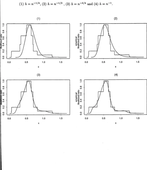
F IG U R E 2.1: U nsm oothed (step function ) via sm oothed em pirical likelihood ratio
functions for m edian based on sam ple
A,
w ith various choices of b an d w id thh:
(1)
h =
n - 1 / 4, (2)h
= n - 1 / 2 . (3)h =
n - 3 / 4 and (4)h = n ~ l .
[image:39.547.8.522.174.766.2]A
= { 0 . 0 1 1 , 0 . 0 2 4 , 0 . 0 5 5 , 0 . 0 6 , 0 . 0 6 8 , 0 . 3 1 3 , 0 . 3 4 1 , 0 . 4 9 6 , 0 . 5 0 6 , 0 . 6 3 3 ,0 . 6 3 9 , 0 . 6 8 9 , 0 . 7 0 , 0 . 8 1 7 , 1 . 2 5 1 , 1 . 2 7 1 , 1 . 4 4 5 , 1 . 6 6 2 , 1 . 6 7 8 }
g e n e r a t e d from t h e \ \ d i s tr i bu ti on .
2 . 3 . 2 W i l k s ’ T h e o r e m a n d C o v e r a g e A c c u r a c y
As p o i n t e d o u t in C h a p t e r 1, a f u n d a m e n t a l result of empir ical likelihood is t h a t , like p a r a m e t r i c likelihood, it a d m i t s a n o n p a r a m e t r i c version of W i l k s ’ t h e o r em. We have m e n t i o n e d in C h a p t e r 1 t h a t th e W i l k s ’ t h e or em holds t r u e for t h e case of s m o o t h f uncti on of m e a n s , which enables us to c o n s t r u c t an empirical likelihood confidence interval by looking up th e chi-square tables. For our c ur r en t p r ob le m of c o n s t r u c t i n g confidence intervals for a quant ile, we would like to first prove t he W i l k s ’ t he or em for ih(6q), which will give us a s m o o t h e d empir ical likeli hood confidence interval with correct a s y m p t o t i c coverage. T h e n we would like to inve st i gat e coverage accur acy a nd B a r t l e t t corr ect abil ity of th e confidence interval. In p a r t i c u l a r , we wish the or d er of m a g n i t u d e of coverage er ror to be of smaller o rd er t h a n n - 1 / 2, which is t he o r d er of t he coverage er ror of u n s m o o t h e d empirical likelihood confidence intervals (as shown in Section 2.2). T h e aim of this s ubsection is to a dd r e s s these pr ob lems by giving t hr ee t h e o re m s ( T h e o r e m s 2.3.3 - 2.3.5). T h e proofs of t he se t h e o r e m s are deferred to Section 2.5.
O u r first result establ ishes necessary and sufficient condi tions on t he choice of b a n d w i d t h , h, such t h a t l h { 0 q) has an a s y m p t o t i c x \ di s t r i b ut i o n.
T h e o r e m 2 . 3 . 3 : A s s u m e that
K satisfies (2.3.1), and is bounded and compactly supported; that
asks t h a t K be a kernel of or de r r. T h e r eq u ir e m e n t s t h a t K be b o u n d e d an d c om p a c t l y s u p p o r t e d implies t h a t Gh is b o u n d e d , so as to get t he result in L e m m a 2.3.2 which is used to prove T h e o r e m 2.3.2. However, we could o b t a i n t he result in T h e o r e m 2.3.2 by impo si ng o t h e r similar co ndi tions on t he kernel. T h e second p a r t asks t h a t t he d i s tr i bu ti on function F be sufficiently s m o o t h in a n e i g h b o u r hood of 6q; t he condi tion t h a t r c ont inuous derivatives of t he t a r g e t f uncti on (here, F) exist is t h e us ual s mo o th n es s a s s u mp t i o n imp os e d when working with an r ’th o rder kernel. Req ui r in g t h a t f ( 9 q) > 0 ensures t h a t t he a s y m p t o t i c variance of th e samp le q u an t il e is of order n ~ 1. W i t h o u t t h a t a s s u m p t i o n t h e or de r of m a g n i t u d e of variance is str ictly larger t h a n n - 1 , and t he a s y m p t o t i c t h e o ry is quit e different. Finally, as king t h a t nh* —> 0 as n —► oo ensures t h a t t he b a n d w i d t h does not co n verge to zero too slowly. Thi s is act uall y a very weak condi tion on h, since t here is no res tr ic ti on on t.
If K is a s econd- or der kernel (i.e. r — 2) and f ' ( 9 q) 0 t h e n t h{ 6q) is a s y m p totically x \ if a n d o n ly if h = o { n ~ ^ ) . Such a b a n d w i d t h is of smal ler or der of m a g n i t u d e t h a n t h a t which is usually a p p r o p r i a t e for mi ni mi si ng error of a curve e s t i m a t o r ; t he l a t t e r h is of size n - ®, as shown for e xa m p l e by Silver man (1986, p.40ff). W h e n f ^ r ~ 1\ 9 q) = 0, it is possible for lh{&q) to have an a s y m p t o t i c x \ d i s t r i b u t i o n yet n h 2r to be b o u n d e d away from zero.
If (2.3.8) is t r u e and we choose the b a n d w i d t h h such t h a t n h 2r —* 0 , t he n by the t he o r e m we can c on s t r u c t an o-level s m o o t h e d e mpir ica l likelihood confidence interval for 6q as follows. F i rs t find from the x \ tables t h e value ca such t h a t
P ( x l < ca ) = a.
Bas ed on T h e o r e m 2.3.3, we a s su me t h a t
n h 2r —► 0 as n —> oo. (2.3.9)
Clearly (2.3.9) implies (2.3.2). To establ ish an expan si on of E d g e w o r t h ty p e for th e d i s t r i b u t i o n f unct i on of i h (9q), we a s su me t h a t
n h / l o g n —> oo, as n —* oo. (2.3.10)
T h e coverage a cc ur acy of I hCa is discussed in th e following th e or em:
T h e o r e m 2 . 3 . 4 : A s s u m e conditions (2.3.8) - (2.3.10). Then a sufficient condition f o r
P ( S , € / » . . ) = a + 0 ( » - ‘ ) (2.3.11) as n —► oo, is that n h r is bounded. This condition is also necessary i f f ^ r ~ 1\ 0 q) ^ 0. T h e o r e m 2.3.4 implies t h a t t he s mo o t h e d empir ical likelihood confidence i n terval I hCa has coverage er r or of or de r n -1 if t h e b a n d w i d t h h is pr op er ly chosen as r e c o m m e n d e d by t he t h e o r e m . Thi s is a significant i m p r o v e m e n t over the u n s m o o t h e d empi ri ca l likelihood confidence interval I Cq given in Section 2.2. Notice t h a t t he b o u n d n e s s of n h r is sufficient for condi tion (2.3.9) to be t ru e. If th e or der of th e kernel K is r > 2, we can choose h = 0 { n ~ l ^r ). It is obvious t h a t for such h, n h r is b o u n d e d a nd n h /log n —> oo. T h e o r e m 2.3.4 assures t h a t this choice of h leads to coverage accur acy of or de r n~ 1.
2 . 3 . 3 . B a r t l e t t C o r r e c t i o n
error by r escaling £h(0q) , so t h a t it has correct me a ns . We s t a r t with cal culating t he e x p e c t a t i o n of £h(9q), which is given in t h e following l e mm a .
L e m m a 2 . 3 . 5 : A s s u m e condi tions (2.3.8) and (2.3.9). Then,
E{ £h{ dq) } = 1 + n ~ 1 ß + n + o ( n h 2r) -f 0 { h 3r + n ~ l h r + n - 2 ) ,
where ß = ^ (3//J 2 /i4 — 2/ig 3 //g) fij = E [ G { ( 9 q —Xt-)/h] — q]j .
We see from L e m m a 2.3.5 t h a t the difference bet ween t h e e x pe c t at i o n s of £h(9q) a n d its a p p r o x i m a t i n g chi-squared d i s t ri b ut io n is d o m i n a t e d by t e rm n ~ l ß + n n \ / i j 1 . So if we choose b a n d w i d t h h such t h a t n h 2r = 0 ( n ~ 2) t h e n we have
E { t h (6q) } - E ( X 2l ) = n - 1 ß + 0 ( n ~ 2).
We m a y r eason t h a t the e x pe c t at i o n of £h{6q)/{ 1 + n ~ l ß ) differs from t h a t of t he Xi d i s t r i b u t i o n only in t e r m s of or der n - 2 , by using b a n d w i d t h h such t h a t n h 2r = 0 ( n ~ 2). However, ß is usually u n k n ow n in pr act ice and m u s t be e s ti m a t e d . To this e n d , we define
n
fij = n - 1 E [G{(#, - * , ) / / * } - ? F
» = 1
an d ß = ^ ( 3 / * "2 — 2f i ~3 /ig), where 9q is a r oo t- n consistent e s t i m a t e of 9q. By
th e s m o o t h n e s s of G and Tayl or expans ion , we ma y show t h a t ß = ß + 0 { n ~ 1^2). P u t d( ca , 7 ) = ca ( l + n- 1 7 ) where 7 is ei t her ß or ß. We prove in th e following
t he o re m t h a t by a p p r o p r i a t e l y choosing h, t he B ar t l e t t - c o r r e c t e d confidence interval
£ h , d ( c a,7 ) = {# I £h(&) ^ d( ca , 7 ) } has s maller coverage er ror t h a n I hCa, no m a t t e r
w h e t h e r ß or ß is used.
T h e o r e m 2 . 3 . 6 . A s s u m e condi tions (2.3.8) and (2.3.10). Then a suffi cient condi tion f or
1*2 = 9 ( 1 - 9 ) + 0 ( h) , V 3 = 9( 1 ~ 9) (1 - 29) + 0 ( h ) ,
A*4 = 9 (1 - 9) (1 - 39 + 392) + 0 ( h ) .
Define ß Q = ^ q ~ 1( 1 — 9)- 1 ( l — 9 + 92)- T h e n we have ß = /30 + 0 ( h ) . Since /30 is k n o w n, a nd if h is small en ou g h, ß 0 will be a good a p p r o x i m a t i o n of ß . For e x a m p l e , if h satisfies t he r eq u i r e m e n t of T h e o r e m 2.3.6 a nd K is a second- or der kernel t h e n ß = ß 0 + 0 ( n - 3 ^4). Define the “p a r t i a l ” B a r t l e t t - c o r r e c t e d confidence int er val Ih,d(ca ,ß0) = {# < ca (1 + ß 0n~ 1) }. It m a y be shown t h a t t he result in (2.3.12) can be changed to
P ( 0 q e I h,d(Ca,0o)) = a + 0 ( n ~ 1 h ) . (2.3.13)
S u pp o s e we use a second or de r kernel and choose th e b a n d w i d t h h of or de r n - 3 / 4, as sug ges ted by T h e o r e m 2.3.6. T h e n we o bt a in
P ( 0 , e / ft,i(c„ , ^ , ) = a + 0 ( n - 7/4).
So t he coverage er r or is j u s t a f actor 0 ( n 1/f4) larger t h a n t h a t of t h e full B a r t l e t t cor rect ion confidence interval.