Nonparametric Bayesian Topic Modelling with Auxiliary Data

(1)

Nonparametric Bayesian Topic

Modelling with Auxiliary Data

Kar Wai Lim

A thesis submitted for the degree of

Doctor of Philosophy of

The Australian National University

(2)

c

2016 Kar Wai Lim

(3)

Except where otherwise indicated, this dissertation is my own original work.

(4)

(5)

Supervisor

Wray Buntine

Professor, Monash University Melbourne, VIC, Australia

Advisors

Edwin Bonilla

Senior Lecturer, The University of New South Wales Sydney, NSW, Australia

Hanna Suominen

Senior Researcher, NICTA

Adjunct Assistant Professor, The Australian National University Professional Associate, University of Canberra

Adjunct Professor, University of Turku (Finland) Canberra ACT, Australia

Scott Sanner

(6)

(7)

(8)

(9)

Acknowledgments

First, I would like to express my deepest gratitude to my supervisor, Wray Buntine, for the support and inspiration during my doctoral study. This dissertation would not be possible if not for his dedication and invaluable advice. I would also like to thank my advisors, Edwin Bonilla, Hanna Suominen, and Scott Sanner, for their comments in and out of research. In addition, I give thanks to the researchers for the interaction through visits and conferences.

My sincere thanks also goes to the Australian National University and NICTA for the financial support by way of a scholarship. In particular, I am grateful to Jochen Renz and Bob Williamson for supporting my application. I also appreciate the various assistance, encouragements, and moral supports from the university staff, NICTA employees, my peers, and my friends. Finally, I thank my family.

NICTA is funded by the Australian Government through the Department of Com-munications and the Australian Research Council through the ICT Centre of Excel-lence Program.

(10)

(11)

Abstract

The intent of this dissertation in computer science is to study topic models for text an-alytics. The first objective of this dissertation is to incorporate auxiliary information present in text corpora to improve topic modelling for natural language processing (NLP) applications. The second objective of this dissertation is to extend existing topic models to employ state-of-the-art nonparametric Bayesian techniques for better modelling of text data. In particular, this dissertation focusses on:

• incorporating hashtags, mentions, emoticons, and target-opinion dependency present in tweets, together with an external sentiment lexicon, to perform opin-ion mining or sentiment analysis on products and services;

• leveraging abstracts, titles, authors, keywords, categorical labels, and the cita-tion network to perform bibliographic analysis on research publicacita-tions, using a supervised or semi-supervised topic model; and

• employing the hierarchical Pitman-Yor process (HPYP) and the Gaussian pro-cess (GP) to jointly model text, hashtags, authors, and the follower network in tweets for corpora exploration and summarisation.

In addition, we provide a framework for implementing arbitrary HPYP topic models to ease the development of our proposed topic models, made possible by modu-larising the Pitman-Yor processes. Through extensive experiments and qualitative assessment, we find that topic models fit better to the data as we utilise more auxil-iary information and by employing the Bayesian nonparametric method.

(12)

(13)

List of Figures

4.1 Graphical Model for the Latent Dirichlet Allocation (LDA) . . . 28

4.2 Graphical Model for the Author-topic Model (ATM) . . . 30

4.3 Graphical Model for the Supervised LDA . . . 31

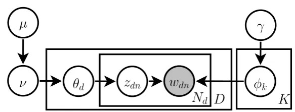
5.1 Graphical Model for the HPYP Topic Model . . . 35

5.2 Chinese Restaurant Process Representation . . . 38

5.3 Chinese Restaurant with Table Multiplicity Representation . . . 39

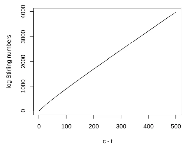
5.4 Plot of Log Stirling Numbers . . . 52

6.1 Graphical Model for the Interdependent LDA . . . 58

6.2 Graphical Model for the Twitter Opinion Topic Model (TOTM) . . . 59

6.3 Preprocessing Pipeline for Tweets . . . 69

6.4 Pairwise Hellinger Distances . . . 75

6.5 Convergence Analysis for the TOTM . . . 78

6.6 The Log Posteriors of the Hyperparameter b . . . 79

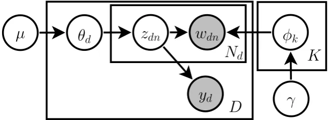
7.1 Graphical Model for the Citation Network Topic Model (CNTM) . . . . 83

7.2 Snapshot of the Author–Topics Network . . . 102

7.3 Training Word Log Likelihood vs Iterations . . . 103

8.1 Graphical Model for the Twitter Network Topic model (TNTM) . . . . 110

8.2 Convergence Analysis for the TNTM . . . 132

8.3 Cumulative Frequency of the Mixing Proportionsρθd0 . . . 133

8.4 Cumulative Frequency of the Mixing Proportionsρθd _{. . . 134}

(20)

(21)

List of Tables

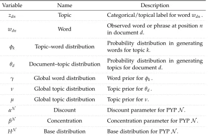
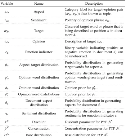
5.1 List of Variables for the HPYP Topic Model . . . 36

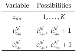
5.2 All Possible Proposals for the Blocked Gibbs Sampler . . . 41

6.1 List of Emoticons and Strong Sentiment Words . . . 60

6.2 List of Variables for the Twitter Opinion Topic Model (TOTM) . . . 62

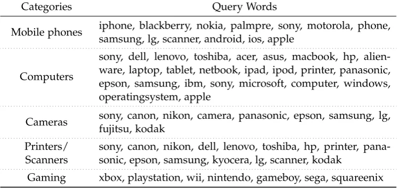
6.3 Keywords for Querying the Electronic Product Dataset . . . 67

6.4 Corpus Statistics . . . 70

6.5 Perplexity Results . . . 72

6.6 Sentiment Classification Results . . . 73

6.7 Sentiment Evaluations for the Sentiment Priors . . . 74

6.8 Top Target Words for the Electronic Product Tweets . . . 75

6.9 Opinion Analysis of Target Words . . . 76

6.10 Aspect-based Opinion Comparisons . . . 77

6.11 Contrasting Opinions on iPhones . . . 78

7.1 List of Variables for the Citation Network Topic Model (CNTM) . . . . 86

7.2 Summary of the Datasets . . . 94

7.3 Categorical Labels of the Datasets . . . 94

7.4 Perplexity for the Training and Test Documents . . . 98

7.5 Comparison of Clustering Performance . . . 99

7.6 Topical Summary for the ML, M10 and AvS Datasets . . . 100

7.7 Major Authors and Their Main Research Area . . . 101

7.8 Time Taken to Perform the Training Algorithm . . . 105

8.1 List of Variables for the Twitter Network Topic model (TNTM) . . . 114

8.2 Keywords for Querying the Datasets . . . 123

8.3 Summary of the Datasets . . . 124

8.4 Test Perplexity and Network Log Likelihood Comparisons . . . 126

8.5 Ablation Test on the TNTM . . . 127

8.6 Clustering Evaluations . . . 129

8.7 Topic Coherence . . . 129

8.8 Topical Analysis of the Learned TNTM . . . 130

8.9 Inference on Authors’ Interest . . . 131

(22)

(23)

List of Acronyms

AG Adaptor Grammars

ASUM Aspect and Sentiment Unification Model ATM Author-Topic Model

BUGS Bayesian Inference Using Gibbs Sampling CAT Citation Author Topic

CNTM Citation Network Topic Model CRP Chinese Restaurant Process DP Dirichlet Process

EM Expectation-Maximisation GEM Griffiths-Engen-McCloskey GP Gaussian Process

HBC Hierarchical Bayes Compiler HDP Hierarchical Dirichlet Process HPYP Hierarchical Pitman-Yor Process IDF Inverse Document Frequency

ILDA Interdependent Latent Dirichlet Allocation JAGS Just Another Gibbs Sampler

LDA Latent Dirichlet Allocation

LDA-DP Latent Dirichlet Allocation with Dirichlet Prior Modified LSI Latent Semantic Indexing

MCMC Markov Chain Monte Carlo

MG-LDA Multi-grain Latent Dirichlet Allocation MH Metropolis-Hastings

ML Machine Learning

NLP Natural Language Processing NMI Normalised Mutual Information PDD Poisson-Dirichlet Distribution

pLSA Probabilistic Latent Semantic Analysis

(24)

xxiv LIST OF TABLES

pLSI Probabilistic Latent Semantic Indexing PMI Pointwise Mutual Information

PMTLM Poisson Mixed-Topic Link Model POS Part-Of-Speech

PYP Pitman-Yor Process

SCNTM Supervised Citation Network Topic Model TF Term Frequency

(25)

Chapter1

Introduction

We live in the information age. With the Internet, information can be obtained easily and almost instantly. This has changed the dynamic of information acquisition. For example, we can now (1) attain knowledge by visiting digital libraries, (2) be aware of the world by reading news online, (3) seek opinions from social media, and (4) en-gage in political debatesviaweb forums. As technology advances, more information is created, to a point where it is infeasible for a person to digest all the available content. To illustrate, in the context of PubMed, a healthcare database, the number of entries has seen a growth rate of approximately 3,000 new entries per day in the ten-year period from 2003 to 2013 [Suominenet al., 2014]. This motivates the use of machines to automatically organise, filter, summarise, and analyse the available data for the users. To this end, researchers have developed various methods, which can be broadly categorised into computer vision [Low, 1991; Mai, 2010], speech recognition [Rabiner and Juang, 1993; Jelinek, 1997], andnatural language processing(NLP) [Man-ning and Schütze, 1999; Jurafsky and Martin, 2000]. This dissertation focuses on text analysis within NLP.

In text analytics, which is often associated with text mining, researchers seek to accomplish various goals, includingsentiment analysis(or opinion mining) [Pang and Lee, 2008; Liu, 2012], topic modelling (or topic segmentation) [Blei, 2012], information retrieval[Manninget al., 2008], andtext summarisation[Lloret and Palomar, 2012]. To illustrate, sentiment analysis can be used to extract digestible summaries or reviews on products and services, which can be valuable to consumers. On the other hand, topic models attempt to discover abstract topics that are present in a collection of text documents. Note that text mining is often associated to the analysis of a large text collection. Since we do not limit our work to only dealing with large text corpora, we will say that this dissertation focusses on topic modelling rather than text mining.

Initially, topic models were developed for unstructured text. Topic models were inspired by the latent semantic indexing (LSI) [Landauer et al., 2007] and its proba-bilistic variant, probabilistic latent semantic indexing(pLSI), also known asprobabilistic latent semantic analysis (pLSA) [Hofmann, 1999]. Pioneered by Blei et al. [2003], the latent Dirichlet allocation(LDA) is a fully Bayesianextension of the pLSI, and can be

(26)

2 Introduction

considered the simplest Bayesian topic model. The LDA is then extended to many different types of topic models. Some of them are designed for specific applications [Wei and Croft, 2006; Meiet al., 2007], some of them model the structure in the text [Blei and Lafferty, 2006; Du, 2012], while some incorporate extra information in their modelling [Ramageet al., 2009; Jinet al., 2011].

This dissertation will concentrate on topic models that take into account addi-tional information. This information can beauxiliary data (or metadata) that accom-pany the text, such as keywords (or tags), dates, authors, and sources; or external resources like word lexicons. For example, on Twitter, a popular social media plat-form, its messages, known astweets, are often associated with several metadata like location, time published, and the user who has written the tweet. This information can also be used. For instance, Kinsellaet al.[2011] model tweets with location data, while Wanget al.[2011b] use hashtags for sentiment classification on tweets. On the other hand, many topic models have been designed to perform bibliographic analy-sis by using auxiliary information. Most notable of these is the author-topic model [Rosen-Zvi et al., 2004], which, as its name suggests, incorporates authorship infor-mation. In addition to authorship, the Citation Author Topic model [Tuet al., 2010] and the Author Cite Topic Model [Katariaet al., 2011] make use of citations to model research publications. There are also topic models that employ external resources to improve modelling. For instance, He [2012] incorporates a sentiment lexicon as prior information into the LDA for a weakly supervised sentiment analysis.

Considering theory, recent advances in Bayesian methods have produced topic models that utilisenonparametricBayesian priors. The most direct approach of these is simply replacingDirichlet distributionsin the LDA byDirichlet process(DP) [Ferguson, 1973], resulting in the hierarchical Dirichlet process LDA (HDP-LDA) proposed by Teh et al. [2006]. One can further extend the topic models by using the Pitman-Yor process (PYP) [Ishwaran and James, 2001] that generalises the DP, this includes Sato and Nakagawa [2010], Du et al.[2012b], Lindseyet al.[2012], among others. Besides more flexible modelling, other advantages of employing the nonparametric Bayesian method on topic models is the ability to infer the number of clusters and to estimate topic prior probabilities from the data. Using PYPs also allows the modelling of power-law properties exhibited by natural languages [Goldwateret al., 2005].

(27)

§1.1 List of Published and Submitted Papers 3

1 .

1 List of Published and Submitted Papers

The following papers are accepted for publication in peer reviewed conference pro-ceedings and journal, listed in reverse chronological order:

1. Lim, K. W., Buntine, W. L., Chen, C., and Du, L. (2016). Nonparametric Bayesian topic modelling with the hierarchical Pitman-Yor processes. Inter-national Journal of Approximate Reasoning, 1(1):1–40.

2. Lee, Y., Lim, K. W., and Ong, C. S. (2016). Hawkes processes with stochastic excitations. In Balcan, M. F. and Weinberger, K. Q., editors, Proceedings of the 33rd International Conference on Machine Learning, ICML 2016, pages 79–88. 3. Lim, K. W. and Buntine, W. L. (2016). Bibliographic analysis on research

pub-lications using authors, categorical labels and the citation network. Machine Learning, 103(2):185–213.

4. Lim, K. W. and Buntine, W. L. (2014). Bibliographic analysis with the Citation Network Topic Model. In Phung, D. and Li, H., editors,Proceedings of the Sixth Asian Conference on Machine Learning, ACML 2014, pages 142–158. Brookline, Massachusetts, USA. Microtome Publishing.

5. Lim, K. W. and Buntine, W. L. (2014). Twitter Opinion Topic Model: Extracting product opinions from tweets by leveraging hashtags and sentiment lexicon. In Li, J., Wang, X. S., Garofalakis, M. N., Soboroff, I., Suel, T., and Wang, M., editors, Proceedings of the 23rd ACM International Conference on Conference on In-formation and Knowledge Management, CIKM 2014, pages 1319–1328. New York City, New York, USA. ACM.

6. Lim, K. W., Chen, C., and Buntine, W. L. (2013). Twitter-Network Topic Model: A full Bayesian treatment for social network and text modeling. In Advances in Neural Information Processing Systems: Topic Models Workshop, NIPS Workshop 2013, pages 1–5. Lake Tahoe, Nevada, USA.

7. Lim, K. W., Sanner, S., and Guo, S. (2012). On the mathematical relationship between expected n-call@k and the relevancevs.diversity trade-off. In Hersh, W. R., Callan, J., Maarek, Y., and Sanderson, M., editors,Proceedings of the 35th International ACM SIGIR Conference on Research and Development in Information Retrieval, SIGIR 2012, pages 1117–1118. New York City, New York, USA. ACM.

The following papers are currently under review:

(28)

4 Introduction

1 .

2 Major Contributions

We outline some major contributions of this dissertation:

1. Framework for Bayesian topic modelling: We present a modelling framework for nonparametric Bayesian topic models that employ the hierarchical Pitman-Yor processes (HPYPs). The novelty of this framework lies in the modularisa-tion of the Pitman-Yor processes (PYPs), allowing us to implement HPYP topic models that are of arbitrary structure. The framework is inspired by BUGS (stands for Bayesian inference using Gibbs sampling) [Lunn et al., 2000], that performs inference on arbitrary Bayesian models. However, BUGS does not extend to nonparametric Bayesian models. Several other tools for automatic in-ference, such as JAGS (stands for just another Gibbs sampler) [Plummer, 2003] and Infer.NET [Minkaet al., 2014], do not work for HPYP topic models.

The above framework has been successfully applied to implement several topic models that will be discussed in this dissertation, like the HDP-LDA,1 a nonparametric extension to the author-topic model (ATM), the proposedTwitter Opinion Topic Model(TOTM), theCitation Network Topic Model(CNTM), and the Twitter Network Topic Model(TNTM). Here we note that the network component of the CNTM and the TNTM is simply implemented on top of the framework, with little modification to the framework.

2. Opinion mining and sentiment analysis: We create a nonparametric Bayesian topic model to perform opinion mining on tweets. The proposed model, TOTM, leverages auxiliary metadata that are present in tweets, such as hashtags, men-tions, emoticons, and strong sentiment words for sentiment analysis. As an extension to theinterdependent LDA(ILDA) [Moghaddam and Ester, 2011], the TOTM models the target-opinion pairs that are extracted from tweets directly. As such, the TOTM is able to discover target specific opinions, which is ne-glected in existing approaches.

Another novelty of this work is a new formulation for incorporating senti-ment prior information into topic models using existing public sentisenti-ment lexi-con. Although there are some existing work [He, 2012; Dinget al., 2008; Taboada et al., 2011] that uses sentiment lexicon for sentiment analysis, their approaches tend to bead hocor rule-based in nature. In contrast, our formulation follows a full Bayesian approach, and it learns and updates itself with the available data.

In addition, we illustrate the usefulness of the TOTM with several quali-tative analysis and applications that cannot be obtained with other topic mod-els. This includes (1) an opinion analysis of specific target words, which are only made possible by modelling the target-opinion interaction directly, (2) an

(29)

§1.2 Major Contributions 5

aspect-based opinion comparison of major brands, and (3) an extract of con-trastive opinions on certain products. We note that this work is published in Lim and Buntine [2014b].

3. Bibliographic analysis: Bibliographic analysis on research publications is al-ways of interest to the research community. For this, we propose the CNTM that models text, the corresponding publication metadata, as well as the associ-ated citation network. Modelling the citation network with a topic model leads to a complicated learning algorithm if we were to apply the standard Markov chain Monte Carlo(MCMC) theory naïvely. Our contribution in this work, apart from designing a full Bayesian topic model for bibliographic analysis, is that we propose a novel and efficient learning algorithm for the CNTM. The proposed algorithm introduces auxiliary parameters and uses the delta method approxi-mation [Oehlert, 1992], to allow some parameters from the network component to be assimilated into the topic model component. Hence, this leads to a sim-pler learning algorithm for the full model.

Moreover, we propose a method to incorporate supervision into the CNTM. This uses the categorical information that is available to the research publica-tions. We demonstrate that incorporating supervision leads to improvement on document clustering. For applications, we use the CNTM for (1) corpora ex-ploration by extracting research topics, (2) analysis of authors’ research areas, and (3) a visualisation of the author-topic network. The work on bibliographic analysis is published in Lim and Buntine [2014a]. An extended version of this work will be available in Lim and Buntine [2016].

4. Bayesian modelling on tweets: We propose a fully Bayesian nonparametric topic model, named the TNTM, to jointly model the text content of tweets, their hashtags, their authors, and the corresponding followers network. The novelty in this work is that the TNTM utilises the HPYP to model the tweets, and the Gaussian process (GP) to model the network. Albeit slightly complicated, the TNTM is carefully designed to model tweets.2 Contrary to some existing topic models that treat hashtags as labels (e.g., Tsai [2011]), we model the hashtags as words that share tokens with text in the tweets. However, they are captured by a different variable. The complexity of the learning algorithm comes from the fact that each PYP in the model can have multiple parent PYPs and that the GP is not a conjugate, thus we develop a sampler that deals with the PYPs in vector form. The main contribution of this work is the holistic model for tweets.

Through experiments, we show that jointly modelling the text content and the followers network leads to an improvement in model fitting, as compared to individual modelling of the text content and the followers network. This

(30)

6 Introduction

supports the argument that the more data the better. On the other hand, ap-plying the TNTM for automatic topic labelling suggests that hashtags are also good labels for topics. This work is published in Limet al.[2013, 2016].

Besides the major contributions mentioned above, in Section 3.2.4, we derive the pos-terior of a hierarchical Dirichlet model in which one of the intermediate Dirichlet distribution is integrated out. We show that this is a mixture ofDirichlet-multinomial distributions. The mixture is linked to the Chinese Restaurant Process (CRP) repre-sentation when we introduce auxiliary variables that select one of the mixture. This result is currently unpublished.

1 .

3 Dissertation Outline

This dissertation is outlined as follows. In Chapter 2, we briefly review the necessary background for Bayesian modelling. In particular, we introduce the terminologies and the basic concepts for Bayesian models. We then discuss some commonly used algorithms for approximate Bayesian inference. We focus on the MCMC method that will be used in this dissertation, the respective algorithms are theMetropolis-Hastings (MH) algorithm and theGibbs sampler.

In Chapter 3, we move on to describe the probability distributions and stochastic processes that we will use in this dissertation. The univariate probability distribu-tions that are mentioned are the Bernoulli distribution, the binomial distribution, and the beta distribution. We discuss the conjugacy of the beta-binomial distribution. We then detail the multivariate counterpart of the above mentioned distributions. Be-sides, we also present a hierarchical Dirichlet model that serves as a simple analogue to the HPYP used in the proposed topic models in later chapters. For stochastic processes, we outline the DP and the PYP, which are the building blocks for the following chapters.

Next, we discuss some commonly used Bayesian topic models in Chapter 4. The simplest of these is LDA. LDA is often extended to more complicated models, a nonparametric extension of LDA is the HDP-LDA. We also discuss topic models that incorporate metadata in their model. Examples are the ATM, the tag-topic model, and the supervised LDA. We also mention some notable and relevant topic models.

Chapter 5 details our topic modelling design and its implementation. We present a generic HPYP topic model that will be extended later. We detail its generation process, its model representation using the CRP metaphor, itsposterior likelihood, and the inference procedure. We then outline some standard evaluations for topic models. The technical details on implementing the topic models are also presented. The discussion on Chapter 5 will be referred extensively by the later chapters.

(31)

§1.4 A Note on Notation 7

TOTM is extended from the generic HPYP topic model and thus the outline in Chap-ter 6 is similar to that of ChapChap-ter 5. In addition, we describe a procedure to incor-porate sentiment lexicon as prior information into topic modelling, which leads to improvement in sentiment classification. Moreover, we discuss the steps to perform data cleaning and preprocessing, which are also relevant for Chapter 7 and 8. We then perform experiments to assess the TOTM and present qualitative results that are made possible with the TOTM. A diagnostic of the TOTM is also presented.

Chapter 7 and 8 follow the same structure as Chapter 6 so we outline the dif-ference. In Chapter 7, we perform bibliographic analysis on research publications with the proposed CNTM. The CNTM is also an extension of the above HPYP topic model. The auxiliary information used by the CNTM includes authors, categories, keywords, abstracts, titles, and the citation network. We propose a novel inference al-gorithm for the CNTM, which combines the network component and the topic model component for efficient learning. Furthermore, we propose a method to incorporate supervision into the CNTM. Experiments show improvement on quantitative evalu-ations and sound qualitative results.

Finally, we propose the TNTM in Chapter 8. The TNTM models the authors, hashtags, and the followers network alongside tweets. Note that rather as labels, the hashtags are treated as words in the TNTM. As with the previous two models, the TNTM is also extended from the HPYP topic model. To model the network, we employ the use of the GP, which leads to a very flexible modelling of tweets. For inference, we propose an MH algorithm to jointly learn the topic model and the follower network. In the experiments, our ablation studies show that each compo-nent of the TNTM is important. We also demonstrate the quality of the TNTM in applications such as topic labelling and analysis of authors. Chapter 9 concludes.

1 .

4 A Note on Notation

Before moving to the next chapter, we discuss the notation philosophy used in this dissertation. We first note that the variables in each chapter are self-contained, that is, we do not carry on the definition of a variable to the next chapter unless explicitly stated. However, we try to keep the meaning of the variables consistent throughout this dissertation. For example, theαandβ in this dissertation are hyperparameters, even though they might not be the same across the chapters.

(32)

(33)

Chapter2

Bayesian Analysis

We first review the necessary background that is relevant to this dissertation. This chapter focuses on the basics of the Bayesian method and we introduce the termi-nologies used later in this dissertation in Section 2.1. Then, in Section 2.2, we present some approximation techniques for Bayesian inference. We will particularly focus on the Markov chain Monte Carlo (MCMC) method as they are employed in this dis-sertation. Examples of the MCMC techniques include the Metropolis-Hastings (MH) algorithm and the Gibbs sampler.

2 .

1 Bayesian Modelling

A classical (frequentist) statistical model treats its parameters as unknownconstants. These parameters need to be estimated by estimatorsthat are usually obtained from techniques such as maximum likelihood estimation and method of moments match-ing.3 _{An estimator is also a}_{statistic, that is, it is a function of the observed data.}

In contrast, a Bayesian model regards its unknown parameters asrandom variables, each of them having a prior distribution of its own. Inference on these parameters are based on their posterior distributions obtainedviathe Bayes’ rule, conditional on the observed data.

An advantage of Bayesian inference over the classical approach is that we can in-corporate our prior knowledge of the parameters into the model, whether the priors are from our own strong beliefs or based on previous experiences. Even when no prior information is available, we can let the priors to be “uninformative” or “vague”, and let the data influence the posterior distributions.

This chapter serves as a refresher on important aspects in Bayesian analysis that are relevant to this dissertation. It is assumed that readers understand the basics of Bayesian methods hence the following discussion will be brief and concise. A

3_{The maximum likelihood estimators refers to the parameter values that maximise the model} like-lihood (or log likelike-lihood), while the estimators from the moments matching method are obtained by matching the theoretical moments with the moment from the data.

(34)

10 Bayesian Analysis

comprehensive review of Bayesian approach can be found in the introductory text Bayesian Data Analysisby Gelman et al. [2013] andBayesian Theory by Bernardo and Smith [1994].

2.1.1 A Simple Model

This dissertation introduces various Bayesian terminologies and concepts by way of a simple Bayesian model, given below:

(y|a,b)_∼ p(y|a,b), (2.1) (a_|b)_∼ p(a_|b), (2.2)

b_∼ p(b), (2.3)

where a, b and y are the random variables of the model, the notation (y|a,b) _∼ p(y_|a,b)means the value ofyfollows aprobability distribution p(y_|a,b)givenaandb.

2.1.2 Priors and Posteriors

In this Bayesian model, a andbare unknown parameters, each having aprior distri-bution; whereas y corresponds to an observable variable. Using the Bayes’ rule, the joint posterior densityof aandbcan be written as

p(a,b_|y) = p(y|a,b)p(a,b)

p(y) , (2.4)

where p(y) =R R

p(y_|a,b)p(a,b)da dbis themarginal probability distributionofy, and p(a,b) = p(a_|b)p(b)is thejoint probability distributionofa andb.

It is more common to write the joint posterior density up to a proportionality,

p(a,b_|y)∝ p(y_|a,b)p(a,b). (2.5) This is because p(y) is often hard to compute (due to the integration) and does not depend on the parameters a and b. Writing the joint posterior density in this proportionality formula allows us to avoid evaluating p(y), but we are still able to analyse the posterior (e.g., using the MCMC method, see Subsection 2.2).

If there is only one parameter of interest to be analysed, we can integrate out the other nuisance parameters to obtain themarginal posterior density. In this case, the marginal posterior densities for parametersa andbare

p(a_|y) =

Z

p(a,b_|y)db, p(b_|y) =

Z

(35)

§2.1 Bayesian Modelling 11

2.1.3 Posterior Inferences

Unlike classical statistics, where inference on the unknown parameters are sum-marised into a single number and its confidence interval, the Bayesian approach enables us to analyse the distributions of the unknown parameters, that is, through the posterior distributions. Nevertheless, it is very useful to look at the key statistics of the posterior distributions, just like the classical approach.

The quantities of interest are posterior mean, median and mode, which are read-ily attainable from the posterior distributions. For confidence interval, a Bayesian equivalent would be the central posterior density region or thehighest posterior density region, for details, see Jaynes and Kempthorne [1976].

In this example, assuming we have seen n values of y, namelyY = (y1, . . . ,yn), the joint posterior distribution can be derived as

p(a,b|Y) = p(Y|a,b)p(a,b)

p(Y) ∝ p(Y|a,b)p(a,b) =p(a,b) n

∏

i=1

p(yi|a,b). (2.7)

Here, we have used the fact that the observed variable y is independent and identically distributed (conditioned on the model parameters a and b). Having the joint posterior, the relevant marginal posterior distributions can then be derived in the usual way.

2.1.4 Predictive Inferences

In addition to obtaining inferences on the model parameters, an important use of Bayesian method is to perform prediction on future data, which is given more em-phasis in practice. Performing predictive inference involves deriving the posterior distribution of the future values, conditioning on the observed data. Such a distribu-tion is named theposterior predictive distribution.

For instance, say, we are interested in predicting a future value of y, denoted as ˜

y; the posterior predictive distribution of ˜y is p(y˜|Y) =

Z Z

p(y,˜ a,b|Y)dadb=

Z Z

p(y˜|a,b)p(a,b|Y)dadb, (2.8) noting that ˜yis conditionally independent of the dataY, conditioned on parameters aandb.

(36)

2 .

2 Approximate Bayesian Inference

Performing Bayesian inference is essentially just analysing the marginal posterior distributions of quantity of interest (parameters, future data, and their functions). A standard approach involves deriving the posterior distributions using the Bayes’ rule and then calculating the statistics of the posterior distributions (such as mean, variance,etc.). Often, deriving the marginal posterior distributions is extremely dif-ficult, if not impossible, that is, there is no closed form solution for the posterior (though using a conjugate prior helps to alleviate the difficulty); this calls for spe-cial techniques to evaluate the posterior distributions, such as numerical integration, however, these can be tedious and time consuming.

Alternatively, MCMC methods are proposed to avoid the need to derive the re-quired marginal posterior distributions [Gelmanet al., 2013]. MCMC methods allow us to sample quantities of interest from the posterior distributions directly and the relevant statistics can be computed from the samples. The merit of MCMC methods comes from the ease of implementing such methods. However, at the expense of longer computation time required to achieve good inference.

If a faster approximation is needed, variational Bayesian methods (or variational inference) [Bishop, 2006] are the next best substitute for MCMC methods. Variational methods can be seen as an extension of the expectation-maximisation (EM) algorithm [Dempsteret al., 1977], as they involve iterative updates of the parametersviaE-steps and M-steps. Despite the increase speed in obtaining the inference, the drawback of using variational approaches is that deriving the needed equations requires great amount of work if not impossible.

This section provides a brief review of MCMC methods as they will be primarily used in the later chapters. Other methods are mentioned, but they are not the focus in this dissertation.

2.2.1 Markov Chain Monte Carlo Methods

The heart of a MCMC method lies in constructing a Markov chain of parameters for which their sampling distributions converge to the desired distributions (in this case the posterior distributions). Hence these samples can be treated as if they are drawn from the posterior distributions directly.

(37)

§2.2 Approximate Bayesian Inference 13

2.2.1.1 Metropolis-Hasting Algorithm

Metropolis-Hasting algorithm was first proposed by Metropoliset al.[1953] and sub-sequently generalised by Hastings [1970]. The MH algorithm only requires that the joint posterior distribution of the model parameters, up to a proportionality con-stant, is known; note that the joint posterior distribution can be easily found using the Bayes’ rule, which is proportional to the prior times likelihood.4

Letθ = (θ1, . . . ,θk)represent a set of parameters having prior distributions given by p(θ) and y = (y1, . . . ,yn) denotes the observed data, assuming the following

simple Bayesian model:

(y|θ)∼ p(y|θ), (2.9)

(θ)∼ p(θ), (2.10)

then the joint posterior distribution is just

p(θ|y)∝ p(y|θ)p(θ). (2.11) Here, we are interested in the marginal posterior distribution p(θ_i|y) and the posterior predictive distribution p(y˜_|y) for future data ˜y, the distribution of inter-est is known as the target distribution. In order to make inference on the quantities of interest, the MH algorithm creates a sequence of random values whose distribu-tions converge to the target distribudistribu-tions. The MH algorithm can be summarised in Algorithm 2.1.

We note that the proposal distributions do not necessarily have to be dependent on any variables in the model. Also note that to accept the candidate value in Step 3(c) in Algorithm 2.1, we would need to generate a uniform random number u be-tween 0 and 1 and accept the candidate value ifu< A0.

With a large sample size R, the distributions of the random samples of θ can be said to converge in distribution to the marginal posterior distributions. To lessen the effect of a potentially badly chosen starting values that might not represent the samples of the posterior distributions, we remove first B sets of samples from the inference, so that the remaining R₋B samples are more appropriate in represent-ing the posterior distributions. Here, B is named burn-in and we say the discarded samples areburned, orburnt.

A drawback of the MH algorithm is that the random values are not truly in-dependent, their correlation comes from the Markov chain method where the next simulated value is obtained from its predecessor. To overcome this, only every other t-th samples (e.g., t =5) are used for the inference; this is called thinning. However, thinning reduces the quality of the inference when the sample size becomes smaller, or leads to a great increase in computational time in order to gather more samples.

(38)

Algorithm 2.1Metropolis-Hasting algorithm

1. Pick initial values for θ = (θ1, . . . ,θk), denote it θ(0) =

θ₁(0), . . . ,θ_k(0)

, which will be the starting point for the Markov chain.

2. Define theproposal distributions(also known as thejumping distributions) for each parameter, f(θ∗_i|y,θ), i=1, . . . ,k, from which the next value forθi is sampled. The proposal distribution is usually chosen such that it is easy to sample and has roughly the same shape as the target distribution.

3. Forr =1, . . . ,R: For j=1, . . . ,k:

(a) Sample a candidate value, θ∗_j from the proposal distribution specified in Step 2 given the other values ofθ:

fθ∗_j y,θ

(r)

1 , . . . ,θ

(r)

j−1,θ

(r−1)

j ,θ

(r−1)

j+1 , . . . ,θ

(r−1)

k

.

(b) Calculate ratio of densities forθ∗_j, defined as

A =

pθ₁(r), . . . ,θ(_j₋r)₁,θ_j∗,θ_j(₊r−₁1), . . . ,θ_k(r−1) y

pθ₁(r), . . . ,θ_j(₋r)₁,θ_j(r−1),θ_j(₊r−₁1), . . . ,θ(_kr−1) y × f θ(_jr−1)

y,θ

(r)

1 , . . . ,θ

(r)

j−1,θ∗j,θ

(r−1)

j+1 , . . . ,θ

(r−1)

k

fθ∗_j y,θ

(r)

1 , . . . ,θ

(r)

j−1,θ

(r−1)

j ,θ

(r−1)

j+1 , . . . ,θ

(r−1)

k .

(c) Update the value ofθ(_jr) to θ_j∗ with acceptance probability A0 = min(A, 1). If θ∗_j is not accepted, then set θ(_jr) = θ(_jr−1), that is, the next value for θj retains the same value.

Note that to make inference on the future data ˜y, we simply generate a sample of ˜y using the simulated parametersθ, the generated ˜ywill be distributed approximately from the posterior predictive distribution. This method also applies to any function of the parameters or any random variable conditioned on the parameters.

2.2.1.2 Gibbs Sampling

(39)

§2.2 Approximate Bayesian Inference 15

the data and all other parameters (except itself):

f(θ∗_i |y,θ) = p(θ∗_i |y,θ₋i), (2.12) whereθ₋i = (θ1, . . . ,θi−1,θi+1, . . . ,θk)is a set of all parameters except forθi.

With this specification of proposal distribution, the acceptance probabilities will be equal to 1; denoting θ(₋r−_i 1) =

θ₁(r), . . . ,θ(_i₋r)₁,θ_i(₊r−₁1), . . . ,θ(_kr−1)

, the acceptance probability for candidate valueθ_i∗ is derived as

A(θ_i∗) =

pθ(₁r), . . . ,θ_it₋₁,θ_i∗,θ_i(₊r−₁1), . . . ,θ(_kr−1) y

pθ₁(r), . . . ,θ_i(₋r)₁,θ_i(r−1),θ_i(₊r−₁1), . . . ,θ_k(r−1) y × p θ_i(r−1)

y,θ

(r)

1 , . . . ,θ

(r)

i−1,θ

(r−1)

i+1 , . . . ,θ

(r−1)

k

pθ_i∗ y,θ

(r)

1 , . . . ,θ

(r)

i−1,θ

(r−1)

i+1 , . . . ,θ

(r−1)

k

=

pθ_i∗ y,θ

(r−1)

−i

pθ(₋r_i−1) y

pθ(_ir−1) y,θ

(r−1)

−i

pθ₋(r_i−1) y

pθ(_ir−1) y,θ

(r−1)

−i

pθ_i∗ y,θ

(r−1)

−i

=1 . (2.13)

Hence under Gibbs sampling, all candidate values are accepted. The Gibbs sam-pler is preferred to the MH algorithm because it produces no wastage(no candidate value is rejected). However, sometimes a considerable amount of effort is needed to derive the distribution of the conditional density and/or to sample from it. Thus there may be a trade-off between efficiency and simplicity.

Note that it is not necessary for us to sample each parameter sequentially (as described above), one can develops an algorithm that updates more than one param-eter at once in each iteration; such MCMC samplers are called blocked Gibbs sampler [Liu, 1994]. Also, in practice we are usually only interested in a certain subset of the parameters and do not care about the others; in such cases we can derive a collapsed Gibbs samplers[Liu, 1994] for which the nuisance parameters are integrated out, doing this requires more effort in derivation but the sampler would be much more efficient.

2.2.2 Other Methods

(40)

Other methods for approximate Bayesian inference includes Expectation Propa-gation [Minka, 2001] and the expectation-maximisation (EM) algorithm [Dempster et al., 1977]. These approaches will not be discussed in this dissertation and we refer the interested readers to the references thereof.

2 .

3 Summary

This chapter reviews some basic of Bayesian methods, including how a Bayesian model is constructed and the how to make inference on quantities of interest in the model. Due to the difficulty to make inference on posterior analytically, which is usually complex in practical situations, various approximation approaches were re-viewed; emphasis was given in the discussion of Markov chain Monte Carlo methods as these will be used primarily in this dissertation.

(41)

Chapter3

Probability Distributions and

Stochastic Processes

This chapter provides a brief review on probability distributions and stochastic pro-cesses. The following illustrated probability distributions and stochastic processes are chosen on the basis of relevance to this dissertation; they are only a tiny portion of all existing (and important) distributions, see Walck [2007] for a comprehensive list of other important probability distributions. We first describe some simple prob-ability distributions in Sections 3.1 and 3.2. Section 3.3 describes the nonparametric approach in Bayesian methods and mentions some stochastic processes.

3 .

1 Univariate Probability Distributions

We first discuss the simple univariate probability distributions. These distributions are characterised by the fact that they generate one variable at a time.

3.1.1 Bernoulli Distribution

TheBernoulli distributioncan be considered as the simplest of all distributions. It is a discretedistribution (i.e., the outcome takes on a fixed value) with only two outcomes: 0 and 1. A classical example having such distribution would be the number of heads obtained from asingletoss of a bent coin.

Letθdenote the probability of landing a head, andxdenotes the number of heads obtained, we say x follows a Bernoulli distribution with parameterθ, which can be presented as follows:

(x_|θ)∼Bernoulli(θ). (3.1) Theprobability density function5associated with xis given by

p(x|θ) =θx(1−θ)1−x, x∈ {0, 1}, θ∈ [0, 1]. (3.2)

5_{It should be called the probability mass function in the case of a discrete probability distribution,} but for convenience, we call it a probability density function as in the continuous case.

(42)

18 Probability Distributions and Stochastic Processes

3.1.2 Binomial Distribution

The binomial distribution is a generalisation of the Bernoulli distribution with mul-tiple trials. Following the above example, if we throw the same bent coin n times and again denote x as the number of heads obtained, then x follows a binomial distribution with parameternandθ:

(x_|n,θ)∼Binomial(n,θ). (3.3) As with the Bernoulli distribution, it is a discrete distribution, but now with (n+1)outcomes fromntrials. The probability density forxis given as

p(x|n,θ) =

n x

θx(1−θ)n−x, x∈ {0, 1, . . . ,n}, θ ∈[0, 1], (3.4) where the notation(n_x)denotes the binomial coefficient, given as

n x

= n!

x!(n−x)!. (3.5)

3.1.3 Beta Distribution

In contrast to the Bernoulli and the binomial distribution, the beta distribution is a continuous distribution (i.e., the outcome can be any real number) for which the outcome can take values between 0 and 1 (inclusive). The beta distribution is usually used as a prior distribution for the probability of an event. For example, we can model the probability of getting a head from a coin toss,θ, by a beta distribution:

p(θ|a,b) = 1 B(a,b)(θ)

a−1₍₁₋

θ)b−1, θ ∈[0, 1], a>0, b>0 . (3.6) Here, the parametersaandbare known as shape parameters, andB(_·,_·)is called the beta function, which serves as a normalisation constant. The beta function can also be written as a product of gamma functions:

B(a,b) = Γ(a)Γ(b)

Γ(a+b) . (3.7)

(43)

§3.1 Univariate Probability Distributions 19

3.1.4 Beta-Binomial Distribution

Consider the following Bayesian model:

(x_|n,θ)∼Binomial(n,θ), (3.8)

(θ|a,b)∼Beta(a,b). (3.9) where aandbarehyperparametersassociated with prior θ. Note that the variablesn, aandbare known (or chosen to be certain values) in the model.

It is not difficult to show that the posterior of θfollows a beta distribution:

p(θ|x,n,a,b)∝ p(x|n,θ)p(θ|a,b)

∝θa+x−1(1−θ)b+n−x−1, (3.10) that is,(θ|x,n,a,b)∼ Beta(a+x,b+n−x). Often times, we rewrite Equation (3.10) as p(θ|x), implicitly conditioning on known variables (n,aandb) for simplicity and ease of reading. This conjugacy also enables us to analytically derive the compound distribution ofx by integrating out the parameterθ:

p(x|n,a,b) =

Z 1

0 p

(x|n,θ)p(θ|a,b)dθ

=

n x

1 B(a,b)

Z 1

0 θ

a+x−1₍₁₋

θ)b+n−x−1dθ

=

n x

B(a+x,b+n₋x)

B(a,b) . (3.11)

This distribution is known as the beta-binomial distribution. Note that the integral in Equation (3.11) is easily computed by recognising that it is part of the posterior distribution ofθ.

For situations where there isa priori ignorance regardingθ (i.e., we do not know whataandbare), three specifications have been proposed: uniformprior (a= b=1), improper prior6 (a = b = 0) and Jeffreys prior (a = b = 1/2). Each of these has its advantages and disadvantages. However, given large sample size (often true for computer science application), the differences between using the three priors tend to be negligible.

Note that the improper prior is not a proper probability distribution in which the density does not sum up (or integrate) to 1. When one uses an improper prior, care must be taken to ensure that the posterior distribution is proper, otherwise the inference obtained is completely useless!

(44)

3 .

2 Multivariate Probability Distributions

Multivariate probability distributions are a generalisation of univariate probability distributions discussed in Section 3.1. The outcomes from a multivariate distribution spans multiple dimensions and their values are often dependent on one another.

As above, this subsection reviews some multivariate distributions that are rel-evant to this dissertation. Again, we refer the readers to Walck [2007] for more information on these distributions and details on the other distributions.

3.2.1 Multinomial Distribution

The multinomial distribution is a multivariate generalisation of the binomial distri-bution. While each binomial trial relates to an event being success (1) or failure (0), a trial in multinomial distribution results in a success in exactly one of k possible outcomes. For example, rolling a die. A sample from a multinomial distribution consists of the frequency of the successes in each outcome afterntrials.

Instead of having a single parameter on probability of success (likeθ in the bino-mial distribution), the multinobino-mial distribution requires parameters in the form of a probability vector (lengthk), which comprises of the probability of getting a success in each outcome. We denote this probability vector asθ = (θ1, . . . ,θk).

Let x = (x1, . . . ,xk) be a vector of frequencies correspond to successes in each outcome afternrolls of ak-sided die (does not need to be a fair die) with the proba-bility of success in each outcome (rolling 1 tok) defined by θ = (θ1, . . . ,θ_k), then the probability density function ofxis

p(x_|n,θ) =

n x

(θ1)x1. . .(θ_k)xk, xi ∈ {0, . . . ,n}, θi ∈[0, 1]. (3.12)

Note that the constraints_∑k_i₌₁xi =nand∑ki=1θi =1 need to be satisfied.

The multinomial distribution is equivalent to the categorical distribution or sim-ply the ‘discrete distribution’ whenn is equal to 1, but the sample space is now one of the possibility (out of k) rather than counts. On the other hand, the multinomial distribution reduces to the binomial distribution whenk=2.

3.2.2 Dirichlet Distribution

(45)

conju-§3.2 Multivariate Probability Distributions 21

gate to the multinomial distribution, exactly like the relationship between the beta distribution and the binomial distribution.

The Dirichlet distribution is parameterised by a vector α = (α1, . . . ,αk)of length k, and has the following probability density function:

p(θ|α) = 1 Bk(α)(θ1)

α1−1_{. . .}₍

θ_k)αk−1_, _θ

i ∈ [0, 1], αi >0 , (3.13) where _∑k_i₌₁θi = 1; Bk(α)is a k-dimensional generalisation of the beta function that normalises the distribution, defined as

B_k(α) = Γ(α1). . .Γ(αk)

Γ(α1+· · ·+αk)

. (3.14)

The Dirichlet distribution can also be parameterised by its meanµand precision

ρ, where ρ = ∑k_i₌₁αi and µ = α/ρ. This parameterisation is sometimes preferred due to its greater interpretability. Like the multinomial distribution, the Dirichlet distribution reduces to the beta distribution whenk=2.

3.2.3 Dirichlet-Multinomial Distribution

Due to the conjugacy of the Dirichlet distribution to the multinomial distribution, a compound distribution named the Dirichlet-multinomial distribution can be con-structed similarly to the construction of the beta-binomial distribution. Specifically, the distribution arises from the following Bayesian model:

(x_|n,θ)∼Multinomial(n,θ), (3.15)

(θ|α)∼Dirichlet(α). (3.16) Again, we can show that the posterior ofθ follows a Dirichlet distribution:

(θ|x,n,α)∼Dirichlet(α+x). (3.17) The parameters α= (α1, . . . ,αk)are also known as pseudocounts as they are added to the observed outcomes. Note that the posterior is simply an empirical distribution of the observed outcomes when an improper prior (where allαi =0) is used.

The probability density function of Dirichlet-multinomial distribution — where the Dirichlet parameter is integrated out — can be derived as

p(x_|n,α) = Z

p(x_|n,θ)p(θ|α)dθ =

n x

1 B_k(α)

Z

(θ1)α1+x1−1. . .(θk)αk+xk−1dθ

=

n x

Bk(α+x)

(46)

We note that if an array of discrete distributions of length n is used instead of the multinomial distribution, that is,(zi|θ)∼Discrete(θ)fori=1, . . . ,n, then

p(z_|n,α) = Bk(α+x)

Bk(α) . (3.19)

The(n_x)term is dropped since the sample space is now consist of all permutations of zinstead of counts.

3.2.4 Hierarchical Dirichlet Model

Consider the following hierarchical Bayesian model in which the prior for a Dirichlet distribution is also Dirichlet distributed:

(x|n,θ)∼Multinomial(n,θ), (3.20)

(θ|α)∼Dirichlet(cα), (3.21)

(α|β)∼Dirichlet(β). (3.22) Here,cis an arbitrary positive constant and βis a positive (non-zero) vector.

From Equation (3.18), we know that the Dirichlet parameter θ can be integrated out, but can we also integrate out the Dirichlet parameter α? Here we show that all Dirichlet parameters in a hierarchical model can be integrated outviathe follow-ing derivation.

p(x|n,β) = Z

p(x|n,α)p(α|β)dα

=

n x

Z _B

k(cα+x) Bk(cα)

1 Bk(β)

k

∏

i=1

(αi)βi−1dα. (3.23)

We can simplify the ratio of the beta functions using the fact that x is a vector of integers, as follows:

Bk(cα+x) Bk(cα) =

∏k

i=1Γ(cαi+xi)

Γ(_∑k_i₌₁cαi+xi)

Γ(∑k_i₌₁cα_i)

∏k

i=1Γ(cαi) = Γ(c)

Γ(c+n) k

∏

i=1

(αi)(αi+1)· · ·(αi+xi−1)

= Γ(c)

Γ(c+n) k

∏

i=1

xi

∑

j=1

Sxi

j (αi)j !

, (3.24)

(47)

§3.3 Stochastic Processes and the Nonparametric Model 23

2012, Theorem 17]. Replacing this formulation into Equation (3.23) gives

p(x|n,β) =

n x

Γ

(c)

Γ(c+n)_t

∑

1,...,tk

k

∏

i=1

Sxi

ti

! 1 Bk(β)

Z k

∏

i=1

(αi)βi+tk−1dα

= n x Γ₍ c)

Γ(c+n)_t

∑

1,...,tk

B_k(β+t) Bk(β)

k

∏

i=1

Sxi

ti . (3.25)

We note thatti is strictly positive whenxiis non-zero, and thetican take values from 1 to xi (inclusive).

From Equation (3.25), we can see that when the Dirichlet parameters are inte-grated out more than once, the distribution corresponds to mixtures of Dirichlet-multinomial distributions. For topic modelling, as we will discuss in later chapters, we can introduce an auxiliary variables called table counts to avoid dealing with the mixtures explicitly. The table counts can be viewed as indicators that select one of the mixture in Equation (3.25). Note that this is consistent with the Chinese Restaurant Process representation that will be discussed in Section 5.3.

Finally, this method can be applied recursively to a deeper hierarchical model of Dirichlet distributions. This gives a more complicated mixtures of Dirichlet-multinomial distributions.

3 .

3 Stochastic Processes and the Nonparametric Model

Astochastic processcan be viewed as an extension of probability distribution, as it is a collection ofrandom variableseach having a probability distribution (which is related to one another). A stochastic process is usually used to represent the evolution of a system (e.g., see Markov chain).

The termnonparametricmodel [Hjortet al., 2010] has two meanings, the first refers to a model that contains no parameters at all, which assumes that data that are observed do not follow a given probability distribution; while the second refers to a model that does not assume a particular structure (i.e., fixed probability distribution), the parameters in this model usually grow in size with the amount of data. In the Bayesian context, the term nonparametric refers to the latter.

This section covers some nonparametric stochastic processes that are related to this dissertation. A review on other stochastic processes is available in Çinlar [2011].

3.3.1 Dirichlet Process

(48)

A sample from a DP is a probability distribution known as theoutput distribution. The support of the output distribution is the same as the base distribution, meaning that a sample drawn from the output distribution must also be possible to be drawn from the base distribution. As with the Dirichlet distribution and beta distribution, the DP is usually used as a prior in a hierarchical Bayesian model.

The DP is formally introduced by Ferguson [1973]. Formally, let H be a random measure on measurable space(_X,_B)and letβto be a positive real number. Gis said to be a DP on(_X,_B)with a base measure H and a concentration parameterβ if for any measurable partition(A1, . . . ,Ak)of X, the distribution of G(A1), . . . ,G(Ak)

is Dirichlet distributed with parameter βH(A1), . . . ,βH(Ak)

:

G∼DP(β,H), (3.26)

then

G(A1), . . . ,G(Ak)

∼Dirichlet βH(A1), . . . ,βH(Ak)

. (3.27)

From this definition, if H is a discrete probability distribution (over a finite space), then the DP is a Dirichlet distribution:

DP(β,H)≡Dirichlet(βH), (3.28) where H= (h1, . . . ,hk)representing a probability vector.

WhenHisnon-discrete(non-atomic, or continuous), a DP is essentially an infinite-dimensional Dirichlet distribution. To draw a sample from the DP, certain sam-pling schemes have been proposed, such as the stick-breaking process [Sethuraman, 1991] and theChinese restaurant process(CRP), which is also known as the Blackwell-Macqueen urn scheme [Blackwell and MacQueen, 1973].

Note that a sample drawn from a DP is always discrete (this does not mean finite) even when the base distribution is continuous. Since in most real world applications a sample from a DP is finite given limited observations, we can treat a DP as a Dirichlet distribution, though using a DP allows us to model an unconstrained (and changeable) number of state space.

3.3.2 Pitman-Yor Process

(49)

§3.3 Stochastic Processes and the Nonparametric Model 25

The PDD is defined by its construction process. For 0≤ α<1 and β> −α, letVk be distributed independently as follows:

(Vk|α,β)∼Beta(1−α,β+kα), fork=1, 2, 3, . . . , (3.29) and define(p1,p2,p3, . . .)as

p1=V1, (3.30)

pk =Vk k−1

∏

i=1

(1−Vi), fork ≥2 . (3.31)

If we let p = (p˜1, ˜p2, ˜p3, . . .) be a sorted version of (p1,p2,p3, . . .) in descending

order, then pis Poisson-Dirichlet distributed with parameterαandβ:

p∼PDD(α,β). (3.32)

Note that the unsorted version (p1,p2,p3, . . .) follows a GEM(α,β) distribution, which is named after Griffiths, Engen and McCloskey [Pitman, 2006].

With the PDD defined, we can then define the PYP formally. Let H be a distri-bution over a measurable space (_X,_B), for 0 _≤ α < 1 and β > −α, suppose that p = (p1,p2,p3, . . .) follows a PDD (or GEM) with parametersα andβ, then PYP is given by the formula

p(x_|α,β,H) =

∞

∑

k=1

pkδXk(x), fork=1, 2, 3, . . . , (3.33)

where X_k are independent samples drawn from the base measureHandδXk(x)

rep-resents probability point mass concentrated atXk (i.e., it is an indicator function that is equal to 1 whenx= Xk and 0 otherwise):

δx(y) = (

1 if x=y

0 otherwise . (3.34)

This construction is named the stick-breaking process. The PYP can also be con-structed using an analogue to Chinese restaurant process (which explicitly draws a sequence of samples from the base distribution). A more extensive review on the PYP is given by Buntine and Hutter [2012].

Nonparametric Bayesian Topic Modelling with Auxiliary Data