Memory, expectation formation and scheduling choices

This is a repository copy of Memory, expectation formation and scheduling choices. White Rose Research Online URL for this paper:

http://eprints.whiterose.ac.uk/90836/ Version: Accepted Version

Article:

Koster, P, Peer, S and Dekker, T (2015) Memory, expectation formation and scheduling choices. Economics of Transportation, 4 (4). pp. 256-265. ISSN 2212-0122

https://doi.org/10.1016/j.ecotra.2015.09.001

© 2015, Elsevier. Licensed under the Creative Commons Attribution-NonCommercial-NoDerivatives 4.0 International http://creativecommons.org/licenses/by-nc-nd/4.0/

[email protected] Reuse

Unless indicated otherwise, fulltext items are protected by copyright with all rights reserved. The copyright exception in section 29 of the Copyright, Designs and Patents Act 1988 allows the making of a single copy solely for the purpose of non-commercial research or private study within the limits of fair dealing. The publisher or other rights-holder may allow further reproduction and re-use of this version - refer to the White Rose Research Online record for this item. Where records identify the publisher as the copyright holder, users can verify any specific terms of use on the publisher’s website.

Takedown

If you consider content in White Rose Research Online to be in breach of UK law, please notify us by

Memory, expectation formation and scheduling choices

Paul Kostera,b,∗

, Stefanie Peerc_{, Thijs Dekker}d a

Department of Spatial Economics, VU University Amsterdam, De Boelelaan 1105, 1081 HV Amsterdam, The Netherlands

b

Tinbergen Institute, Gustav Mahlerplein 117, 1082 MS Amsterdam, The Netherlands

c

Vienna University of Business and Economics, Welthandelsplatz 1, 1020 Vienna, Austria

d

University of Leeds, Institute for Transport Studies, 36-40 University Road, Leeds, LS2 9JT, UK.

Abstract

Limited memory capacity, retrieval constraints and anchoring are central to expectation for-mation processes. We develop a model of adaptive expectations where individuals are able to store only a finite number of past experiences of a stochastic state variable. Retrieval of these experiences is probabilistic and subject to error. We apply the model to scheduling choices of commuters and demonstrate that memory constraints lead to sub-optimal choices. We analytically and numerically show how memory-based adaptive expectations may sub-stantially increase commuters’ willingness-to-pay for reductions in travel time variability, relative to the rational expectations outcome.

Article published as: Koster, P., Peer, S. and Dekker,T. (2015). Memory, expectation formation and scheduling choices. Economics of Transportation.

http://dx.doi.org/10.1016/j.ecotra.2015.09.001

Keywords: Memory, Transience, Expectation formation, Adaptive expectations, Retrieval Accuracy, Scheduling, Value of Reliability

I_{We like to thank two anonymous referees for very helpful suggestions for improvements. The paper also} benefited from suggestions and comments of Alexander Muermann, Hans Koster, Peter Nijkamp, participants of the 2014 conference of the European Association for Research in Transportation (hEART) in Leeds, participants of the 2014 conference of the International Transportation Economic Association (ITEA) in Toulouse, participants of a TLO seminar at Delft University. Paul Koster gratefully acknowledges the financial support of the ERC (Advanced Grant OPTION # 246969).

∗

Corresponding author. Fax +31 20 5986004, phone +31 20 5984847.

Email addresses: [email protected](Paul Koster),[email protected](Stefanie Peer),

1. Introduction

Imperfect knowledge regarding the true distribution of stochastic state variables, like prod-uct quality or travel times, induces individuals to form expectations based on personal experiences and external sources of information. Memory processes are known to influence expectation formation processes (e.g.Hirshleifer and Welch,2002;Mullainathan,2002; Wil-son, 2003; Sarafidis, 2007) and anchoring constitutes a persistent phenomenon in human behaviour (Wilson et al., 1996; Strack and Mussweiler,1997; Furnham and Boo, 2011).1

This paper develops an adaptive expectations model which explicitly accounts for limited cognitive abilities of decision makers. Expectation formation in our model has the following properties. First, decision makers are assumed to have limited memory, such that only a fixed number of past experiences can be stored. Second, retrieving experiences from memory is probabilistic and decision makers experience difficulty in retrieving more distant experiences; a phenomenon often referred to as transience (Horowitz,1984;Barucci,1999,2000;Schacter, 2002). Third, retrieval may be inaccurate, meaning that retrieved experiences may not correspond to the original experiences. Transience and retrieval inaccuracy are both forms of memory decay. Fourth, decision makers prime their expectations using exogenous anchors. The inclusion of past experiences, limited cognitive abilities and anchoring in the expectation formation model provides a significant deviation of the rational expectations model.

We apply the model to scheduling decisions of commuters facing stochastic daily travel times. Commuters experience dis-utility from travel time variability, as it induces them to depart and/or arrive earlier or later than preferred (e.g. Vickrey, 1969; Small, 1982, 1992; Noland and Small, 1995). The developed model provides a better understanding of empirical findings that hint at the presence of adaptive expectations and anchors in the context of travel related scheduling decisions. For example, Bogers et al. (2007) and Ben-Elia and Shiftan(2010) provide evidence that recently experienced travel times have an over-proportionally large influence on travel decisions. Peer et al. (2015) find that commuters take into account the long-run travel time average as well as day-specific traffic information in their scheduling decisions.

The value commuters attach to a marginal reduction in travel time variability is referred to as the value of (travel time) reliability and can be inferred from observed scheduling choices (Fosgerau and Karlstr¨om, 2010;Fosgerau and Engelson, 2011). Typically, the value of reliability is derived using the presumption that commuters have rational expectations and an infinite memory. We find that with adaptive travel time expectations this value of reliability is higher, because sub-optimal scheduling decisions are made. Therefore, im-provements in reliability are associated with larger benefits, because they make commuters depart and arrive closer to the times they prefer and decrease the variability in departure times. Empirical revealed preference studies using reduced-form utility functions are likely to already capture these behavioural biases in the coefficient that is estimated for travel

1_{Often anchors corresponds to the information that is obtained first, which is then used as a reference}

time variation. Our results are therefore mainly important for current stated preference practice that ignores the process of expectation formation: our numerical illustration shows that these values of reliability can underestimate our bounded rationality value of reliability by up to 45%, suggesting that the welfare effects of memory biases may be substantial.

Underestimation of the value of reliability may have significant implications for cost-benefit assessments of transport policies. Namely, the cost-benefits from improvements in travel time reliability in road-related transport projects amount to ca. 25% of the benefits related to travel time gains (Peer et al.,2012). Benefits from travel time gains, in turn, are estimated to constitute on average 60% of total user benefits in transport appraisals (Hensher,2001). While we apply our model to scheduling choices of commuters, it may very well be relevant to other fields of economics, such as for the study of the effects of heterogeneous ex-pectation formation on (dis)equilibrium in dynamic economic systems (seeHommes (2013)) or for the analysis of repetitive consumer choices with uncertain product quality. Note that bounded rationality in our model is exclusively caused by limited cognitive abilities rather than judgement errors due to selective memory (Gennaioli and Shleifer,2010) or probability weighting. Therefore this paper stands apart from works modelling bounded rationality as a result of satisficing (Simon, 1955; Caplin et al., 2011), self-deception (B´enabou and Ti-role, 2002), or optimal belief formation when the decision utility is affected by anticipatory emotions (Brunnermeier and Parker, 2005; Bernheim and Thomadsen, 2005) as well as by (ex-post) disappointment (Gollier and Muermann,2010).

The remainder of the paper is structured as follows. Section 2 describes the general setup of the model, Section 3 applies that model to the specific case of scheduling decisions. Section 4 provides numerical estimates of the biases that may result from memory limitations and anchoring. Finally, Section 5 discusses the modelling assumptions and concludes.

2. General description of the model

Consider a decision-maker who decides on x0, where the subscript 0 indicates that the

decision is made for the time period to come. Outcome utility U(x0, s0) is assumed to be

continuous and strictly concave inx0, and depends on the stochastic states0. Letf(s0|ω0) be

the probability density function ofs0, where ω0 is a vector of parameters that characterizes

f(.). Expected outcome utility is then defined as:

E_{(U(x0, s0)) =}

Z

U(x0, s0)f(s0|ω0)ds0 (1)

With rational expectations, the decision maker knows the distribution f(s0|ω0) and

maxi-mizes Equation1to decide onx0. In what follows, we denotexre0 as the optimal choice under

rational expectations, and E_{(Ure) ≡} E_(U(xre

0 , s0)) as the corresponding maximal expected

utility. Deviations from rational expectations are introduced by assuming that the decision maker has imperfect knowledge regarding f(s0|ω0). In our model, she forms adaptive

ex-pectations regarding s0, using past experiences in combination with primed expectations.

f(sk|ωk). A higher value of the index k refers to a more distant experience. Primed

expec-tations enter the model in the form of an anchor state sA. In contrast to the states stored

in the decision maker’s memory and the corresponding retrievals, the anchor is assumed to be non-stochastic and is a stable element in the expectation formation process.

The decision maker is assumed to have limited cognitive abilities. First, it is assumed that she has a limited memory, meaning that only K past experiences s1...sK are stored

in memory. Second, it is assumed that the realisation of sk is correctly stored in memory,

but a stored state can only be retrieved with a probability ρk > 0. Following Schacter

(2002), this allows us to assume that more recent experiences can be retrieved more easily, i.e. ρ1 > ρ2 > ... > ρK. We refer to this phenomena as transience. Third, retrieval of

the stored states s1...sK may be inaccurate. Instead of s1...sK, the decision maker retrieves

¯

s1...¯sK from her memory. Let gk(¯sk|sk, φk) be the retrieval density function, with φk and

sk as its characterizing parameters. Fourth, anchoring is present. The anchor reflects an

exogenous, stable belief concerning travel time that is independent of new experiences and the current traffic situation. While we do not model the origin of the anchor explicitly in order to keep the model generic, the anchor could for example be driven by stable publicly available information.

Equation2defines the expected decision utility as the weighted average of utilities across the anchor and the set of retrieved states:

Ud(.) =τ U(x0, sA) + (1−τ) K X

k=1

ρkU(x0,s¯k), (2)

where PK

k=1ρk = 1. In this equation,τ is the weight assigned to the anchor. When τ = 0,

expectations are fully adaptive and when τ = 1, the decision maker ignores her earlier experiences and expected decision utility is solely based on the anchorsA and the choice of

x0. Equation 2 mimics Equation 1 when τ → 0,ρk = 1/K, ¯sk =sk and K → ∞. Rational

expectations are therefore a special case of our model. The decision maker maximizes Equation 2 with respect to x0. Denote this optimal x0 by xae0 , where the ae superscript

refers to the fact that the decision maker uses adaptive expectations.2 _{Decisions on x}

0 are

sub-optimal whenever xae

0 6= xre0 . Nevertheless, the situation could arise where xae0 = xre0 ,

i.e. the decision maker ’coincidentally’ makes the optimal choice.

Suppose that we need to make a prediction of the expected outcome utility of the decision maker. This prediction has to account for the fact that the state in time period 0, the states in memory and the corresponding retrievals of these states are stochastic. To obtain the predicted expected outcome utility, we take the expected value over all possible combinations of experienced and retrieved states. Mathematically this is tedious, since it involves a 2K+1 dimensional integral over all possible values of the K+ 1 realised states s0...sK, and the K

2_{A unique solution for x}ae

possible values of retrieved states ¯s1...¯sK:

E_(Uae)≡E_(U(xae

0 , s0))

=

Z

...

Z Z

...

Z

U(xae₀ , s0)

K Y

k=1

gk(¯sk|sk, φk)d¯s1...¯sK)

! _K

Y

k=0

f(sk, ωk)ds0...dsK.

(3)

This equation obviously has the disadvantage that it is less parsimonious than its rational expectations counterpart, i.e. Equation1withxre

0 . Nevertheless, this generic set-up helps to

structure our thoughts about how earlier experiences and retrieval inaccuracy affect predic-tions of the expected outcome utility. The next section makes analytical progress by putting more structure on the utility function U(.) and derives an analytical representation of the predicted expected outcome utility E_{(Uae) for the case of commuters choosing departure}

times when travel times are stochastic.

3. Memory and the value of travel time reliability

We apply our memory-based adaptive expectation formation model to commuters’ schedul-ing behaviour with stochastic travel times. Commuters face schedulschedul-ing costs of travel time variability due to departing and/or arriving earlier or later than desired. Noland and Small (1995) were the first to extend the scheduling model ofVickrey (1969) andSmall (1982) to expected utility maximization. Their model was recently extended by Fosgerau and Karl-str¨om (2010) and Fosgerau and Engelson (2011) who proved that the optimal expected outcome utility depends linearly on some measure of travel time reliability. Here, we ex-tend the results of Fosgerau and Engelson(2011) by showing that this result carries over to the case when memory biases and anchoring are present and the travel time distribution is stable over time. Existing literature on travel time expectation formation typically focuses on learning and perception updating mechanisms in route choice but often ignores the psy-chological foundation of the adaptation of expectations (e.g. Jha et al., 1998; Arentze and Timmermans, 2003;Chen and Mahmassani, 2004;Avineri and Prashker, 2005;Arentze and Timmermans, 2005;Bogers et al.,2007;Ben-Elia and Shiftan,2010). Moreover, most exist-ing studies do not quantify behavioural and valuation biases, even when they find that travel time expectations are adaptive. Therefore it is unclear if choice models assuming rational expectations can be viewed as a good approximation of individual choice behaviour. This paper explicitly focuses on the origins of adaptive travel time expectations and characterizes the resulting behavioural and valuation biases.

3.1. Rational expectations

travel time variance. Tseng and Verhoef (2008) were the first to find empirical evidence for such scheduling preferences.

Equation4describes outcome utility for a given departure timed0 and a realisation of travel

time T0, where H′(v) is the marginal utility for being at home and W′(v) is the marginal

utility for being at work as functions of clock time v. The first part of Equation 4 shows the utility from time spent at home where being at home starts at vh and ends when the

travellers departs atd0. The second integral gives the utility for being at work, where being

at work starts at arrival timed0+T0 and ends at vw. This implies that vh and vm span the

range of possible departure and arrival times (B¨orjesson et al. (2012)).3

V(d0|T0) =

Z d0

vh

H′

(v)dv+

Z vw

d0+T0

W′

(v)dv=H(d0)−H(vh) +W(vw)−W(d0+T0). (4)

For the remainder of the paper we assume simple linear functional forms for the marginal utilities. Using the normalisation of B¨orjesson et al. (2012) we have:4

U(d0|T0) =−

Z 0

d0

(β0+β1v)dv−

Z d0+T0

0

(β0+γ1v)dv. (5)

For a trip to occur it must hold that γ1 > β1. Usually the marginal utility of being at

home is decreasing in v, implying β1 <0, whereas the marginal utility of being at work is

increasing (γ1 >0). With rational expectations, commuters know the distribution of travel

times which is defined byf(T0|µ, σ2), whereµis the mean travel time andσ2 the travel time

variance. Accordingly, the expected outcome utility is defined by:

E_{(U(d0|T0)) =}

Z

U(d0|T0)f(T0|µ, σ2)dT0. (6)

Fosgerau and Engelson (2011) show that when the departure time is optimally chosen, the commuter departs at:

dre

0 =−

γ1

γ1−β1

µ, (7)

resulting in optimal expected outcome utility:

E_(Ure)≡E_(U(dre

0 |T0)) = −β0µ+

1 2

β1γ1

γ1−β1

µ2− 1

2γ1σ

2_{. (8)}

3_{For a graphical representation we refer to Tseng and Verhoef (2008), Fosgerau and Engelson (2011)} andB¨orjesson et al.(2012).

4_{Following B¨orjesson et al. (2012), we normalise utility relative to V(0|0), by defining U(d}

0|T0) =

V(d0|T0)−V(0|0). This allows us to evaluateU(d0|T0) in terms of bounds at 0 rather than atvh andvm:

U(d0|T0) =−

Z 0

d0

H′

(v)dv−

Z d0+T0

0

W′

(v)dv=H(d0)−H(0) +W(0)−W(d0+T0)

Furthermore, we normaliseW(0)−H(0) to 0, because this part of utility is independent of departure time

This optimal expected outcome utility is a simple function of the mean delay and the travel time variance. Equation 8 does not require any distributional assumptions on the travel time distribution (except that µandσ2 _{are finite). We define the value of reliability (VOR)}

as the value attached to a marginal decrease in the travel time variance:5

VORre =−

∂E_(Ure)

∂σ2 =

1

2γ1. (9)

3.2. Adaptive expectations

Adaptive expectations on the distribution of travel times are based on past travel times stored in memory T1...TK and the retrievals of these past states ¯T1...T¯K. Every retrieval

is assumed to be an additive function of the retrieval error and the realised travel time: ¯

Tk =Tk+ǫk, with E(ǫk) = 0, meaning that retrieval is on average correct. The travel times

in memory are realizations from f(Tk|µ, σ2). The accuracy of retrieval ǫk is governed by

the probability density functiong( ¯Tk|Tk, νk2) where ¯Tkhas meanE( ¯Tk) = Tk and conditional

variance VAR_{( ¯Tk|Tk) = ν}2

k. Using the law of total variance, the unconditional variance

of ¯Tk is given by: VAR( ¯Tk) = σ2 + νk2.6 For every day t the commuter has to decide

on the departure time and creates a new set of recalled memories from the stored set of past experiences. For large K, the set of past travel time experiences stored in memory for days t and t+ 1 is nearly identical as the experienced travel time at t only replaces a single experience previously stored in memory. The similarity in available memories in combination with transience introduces correlation in the recalled sets, but the process of the recollection and accuracy of these recollections are completely independent between t and t+ 1.

The commuter has an anchor TA which is defined as: TA = µ+a, where a is a

pa-rameter that indicates how far the anchor is from the mean travel time µ. With adaptive expectations, commuters choose their optimal departure using decision utility

Ud(.) = τ U(d0, TA) + (1−τ) K X

k=1

ρkU(d0,T¯k), (10)

wherePK

k=1ρk = 1. Solving the first-order condition ∂Ud

(.)

∂d0 = 0 gives:

dae₀ =−τ γ1 γ1−β1

TA−(1−τ)

γ1

γ1−β1

K X

k=1

ρkT¯k. (11)

5_{For plausibility of the model, additional restrictions may be imposed because for some combinations}

of preference parameters the marginal utility for changes in the mean delay−β0+_γβ11−γβ11µmay be positive,

implying that increases in mean travel time would lead to a higher expected utility. 6 _{We assume COV(T}

The effect of the anchor on departure time choice is captured by the first term, and the effect of limited memory by the second term. A higher K indicates that the commuter is able to store more past travel times. Stored travel times are retrieved with probability ρk.

Retrieval accuracy enters the departure time choice via the retrieved travel times ¯Tk. The

mean departure time is given by:

E_(dae

0 ) =−τ

γ1

γ1−β1

TA−(1−τ)

γ1

γ1−β1

µ, (12)

which reduces to dre

0 for TA = µ (a = 0) (see Equation 7). The variability in departure

time choices over time periods is influenced by the variance of travel times and the variance of retrieval inaccuracy. A higher variance in travel times and a higher retrieval inaccuracy result in more variable departure times:7

VAR_(dae

0 ) = (1−τ)2

γ1

γ1−β1

2

σ2

K X

k=1

ρ2k+ K X

k=1

ρ2kνk2 !

. (13)

Our model therefore predicts that the variability in departure times increases for increasing variances of travel time and retrieval. This effect is multiplied with the quadratic retrieval probabilities. When transience is stronger, retrieval probabilities will be more unequal, resulting in more volatile behaviour. A higher anchor parameter τ results in less variable departure times because memory biases count less heavily in the decision utility function. The prediction of the expected outcome utility can be found by integrating over all possible combinations of T0, T1...TK and the corresponding stochastic retrievals ¯T1...T¯K (i.e. in a

similar way as Equation 3). In Appendix A we show that the predicted expected outcome utilityE_{(Uae) can be written as:}8

E_{(Uae) =}E_(Ure)− 1

2 γ2

1

γ1 −β1

τ2a2− 1

2(γ1−β1)VAR(d

ae

0 )

=E_(Ure)− 1

2 γ2

1

γ1 −β1

τ2a2− 1

2(1−τ)

2 γ12

γ1−β1

σ2

K X

k=1

ρ2k+ K X

k=1

ρ2kνk2 !

.

(14)

The first term in Equation 14 is the optimal expected utility with rational expectations (Equation8). The second term reflects a penalty for relying on an anchor when deciding on the optimal departure time. This penalty only arises when a 6= 0, and increases quadrati-cally in the value of a and the anchor parameter τ. When τ → 1 and TA=µ, the optimal

departure time Equation 11 is equal to the departure time with rational expectations and Equation 14reduces to Equation 8.

7_{Here we use the assumptions on covariances in footnote6. When relaxing these assumption additional} covariance terms would enter this equation.

Adaptive expectations are associated with an additional term that is proportionally decreas-ing in the variance of departure timeVAR_(dae

0 ). More volatile behaviour therefore decreases

the predicted expected outcome utility. First, an increase in the travel time variance results in additional dis-utility because of limited memory. Second, K enters the summation over all retrieval variances νk. Accordingly, the retrieval variances of the last K time periods

decrease expected outcome utility. The negative effect of transience and inaccurate retrieval becomes stronger when commuters’ expectations become more adaptive (i.e. when τ de-creases).

Equation 14is derived for general values of retrieval probabilities, travel time variance and retrieval variances. When imposing transience, we have ρ1 > ρ2 > ... > ρK, such that more

recent travel time and retrieval variances play a larger role than more distant travel time and retrieval variances in Equation 14. Because retrieval probabilities enter quadratically, transience always reduces utility when retrieval is accurate. However, when retrieval vari-ances are high for more distant memories (i.e. higher values of k), transience may reduce the bias of inaccurate retrieval.

The anchor parameter τ has two roles in Equation 14. Given TA 6= µ, an increase in τ is

associated with a decrease in expected utility due to the sub-optimal choice of TA. On the

other hand, an increase in τ may lead to a decrease in the bias related to transience and retrieval inaccuracy, since past experiences have a lower effect on travel time expectations. 3.3. The value of travel time reliability

The VOR with adaptive expectation is given by:

VORae =−

∂E_(Uae)

∂σ2 =

1 2γ1+

1 2

γ2 1

γ1−β1

(1−τ)2

K X

k=1

ρ2_k, (15)

where it is assumed thatτ is exogenous. As with rational expectations (see 9), the expected outcome utility is linearly decreasing in the travel time variance. The convenient result of Fosgerau and Engelson(2011) thus carries over to the case of adaptive expectations. While the VOR is not affected by retrieval inaccuracy, it is affected by transience and the anchor weightτ. Regardingτ, it is easy to see that the VOR increases as the weight attached to the anchor decreases and expectations thus become more adaptive. Clearly, ifτ →1 (and hence only the anchor counts), the VOR is not any longer affected by the transience parameterρk.

It is useful to parametrize the retrieval probabilities. These probabilities need to sum up to 1 for any chosen value of K = 1...∞, and for transience to apply, the probabilities need to be decreasing ink, because more recent travel times will then have a higher likelihood of being remembered. A functional form that satisfies these conditions is given by:

ρk =

r−1 r(rK₋₁₎r

k

, (16)

1

K are a limiting case, because limr→1ρk = _K1. If we assume that retrieval probabilities are

defined by Equation16, the VORae is given by:

VORae,r =

1 2γ1+

1 2

γ2 1

γ1−β1

(1−τ)2(1−r)(1 +r

K₎

(1 +r)(1−rK₎, (17)

which is decreasing in the transience parameter r, meaning that more unequal retrieval probabilities increase the value attached to reliable travel times. The limiting case r → 1 gives retrieval probabilities equal to 1/K. The value of travel time variance is then given by

lim

r→₁VORae,r =

1 2γ1+

1 2

γ2 1

γ1−β1

(1−τ)2 1

K, (18)

and therefore in the absence of transience the additional effect of limited memory on the VORae is proportional to _K1. As expected, the behavioural bias due to limited memory then

vanishes when K → ∞, and VORae,r reduces to 9.

3.4. The value of retrieval accuracy

The expected outcome utility (see Equation 14) shows that it is valuable for commuters to have a higher accuracy of retrieval. The value of retrieval accuracy (VORA) for retrieval m is defined as the first derivative of Equation14 with respect toν2

m, multiplied by (−1):

VORAm =−

∂E_(Uae)

∂ν2

m

= 1 2

γ2 1

γ1−β1

(1−τ)2ρ2m,∀m= 1...K. (19)

The VORA increases when expectations become more adaptive (τ → 0), and when that particular experience has a larger impact on the expected outcome utility. A more explicit expression can be derived by replacingρm in Equation 19by Equation 16:

VORAm,r =

1 2

γ2 1

γ1−β1

(1−τ)2

r−1 r(rK ₋₁₎r

m

2

,∀m = 1...K. (20)

In line with intuition, when transience is present, the VORA is lower for more distant memories (higher m). This illustrates the interesting interplay between transience and the effects of retrieval inaccuracy.

3.5. The limiting case of K → ∞ and ν2

k →νk¯

This subsection develops a limiting case that may be useful for practical applications. It is assumed that memory is unlimited and that an infinite number of experiences are stored. Furthermore, it is assumed that the retrieval variance is linearly increasing in k with slope ¯

ν:

If we substitute Equations16and21in Equation14we obtain a parsimonious expression for the expected outcome utility under infinite memory as a function of the transience parameter r and retrieval variance parameter ¯ν9_:

E_{(Uae) =}E_(Ure)−1

2 γ2

1

γ1−β1

τ2a2−1

2 γ2

1

γ1−β1

(1−τ)21−r 1 +rσ

2

−1

2 γ2

1

γ1−β1

(1−τ)2 ν¯ (1 +r)2.

(22)

The biases due to transience and inaccurate recall do not vanish when memory capacity is unlimited. Equation 22 does show that when the retrieval probabilities are all equal (r → 1), the third term drops out, and the transience bias vanishes, but the bias due to retrieval inaccuracy does not. Accordingly, infinite memory is not a sufficient assumption for rational expectations.

3.6. Endogenous choice of τ

This section generalizes the model to allow for the choice of the anchor parameter, which corresponds to the situation where the decision-maker is aware of her memory limitations. Fora6= 0, the decision-maker will trade-off the bias related to the anchor with the memory biases. The change in expected utility for a marginal change in τ is given by:

∂E_(Uae)

∂τ =− γ2

1

γ1−β1

τ a2+ γ

2 1

γ1 −β1

(1−τ) σ2

K X

k=1

ρ2_k+

K X

k=1

ρ2_kν_k2

!

. (23)

Solving the first-order condition ∂E(Uae)

∂τ = 0 results in:

τ∗

=

PK

k=1ρ2kσ2+

PK

k=1ρ2kνk2

PK

k=1ρ2kσ2+

PK

k=1ρ2kνk2+a2

(24)

which is equal to 1 ifa= 0, and independent of scheduling preferences. The optimal anchor parameter weighs the dis-utility related to imprecision due to anchoring with the dis-utility related to memory biases. Incorporating an anchor (i.e. τ∗

6

= 0) is therefore a rational response to cope with imprecision in knowledge about the true distribution. An increase in σ2 _{will result in an increase inτ}∗

, because – as a consequence of the severity of the memory biases – the decision-maker will rely more on her anchor:

∂τ∗

∂σ2 =

a2PK k=1ρ2k

PK

k=1ρ2kσ2+

PK

k=1ρ2kνk2 +a2

2 >0. (25)

9_{For the limiting case of K → ∞ we have:} P∞

k=1ρ2k = 1

−r 1+r and

P∞

k=1ρ2kνk¯ = (1+ν¯r)2, resulting in a

A marginal upward change in τ∗

results in a higher bias due to anchoring and a lower bias due to transience and retrieval inaccuracy. In Appendix B we show that these marginal changes cancel each other out, resulting in a value of reliability of:

VORae,τ∗ =

1 2γ1+

1 2

γ2 1

γ1−β1

(1−τ∗

)2

K X

k=1

ρ2k

= 1 2γ1+

1 2

γ2 1

γ1−β1

a4PK k=1ρ2k

σ2PK

k=1ρ2k+

PK

k=1ρ2kνk2+a2

2.

(26)

The last step uses Equation24. The second positive term captures the combined dis-utility for anchoring and memory biases (i.e. transience and retrieval inaccuracy). For a = 0, the VOR reduces to the rational expectations case of Equation 9 because the decision-maker then fully relies on the anchor (see Equation 24). This results in a departure time choice that coincides with the rational expectations case (see Equations 7 and 11). The VOR is now decreasing in the travel time variance, because the second term is lower for higher values of σ2_{. The convenient result that expected utility is linear in travel time variance therefore}

does not hold any longer when the anchor parameter is endogenous.

4. Numerical illustration

This section provides a numerical illustration to investigate the quantitative impact of mem-ory biases. We present results for four parameters, namely r, τ, TA, and ¯ν, and trace their

impacts on optimal departure times, expected utility and the value of travel time reliability. The rational expectation levels of these measures (as defined in Section4.1) are used as the point of reference. Section 4.2 analyses the effect of transience by reducing the value of r such that expectations are increasingly based on recent experiences. At this stage, retrieval is assumed to be accurate. Section 4.3 maintains this assumption but introduces anchoring by increasing the value of τ and varying the value TA = µ+a. Section 4.4 completes the

numerical analysis by introducing inaccurate retrieval. Finally, Section 4.5 summarizes the results of the numerical analysis.

4.1. Parameter assumptions and the rational expectations outcome

The values for the coefficients defining the rational expectations outcomes of the model are based on Tseng and Verhoef (2008) and Fosgerau and Lindsey (2013). Accordingly, β0, β1

andγ1 take the following values: β0 =AC40 (p/hour),β1 =AC8.86 (p/hour) andγ1 =AC25.42

(p/hour). We use the empirical estimates ofPeer et al.(2012) to parametrize the distribution of travel times. We assume that f(Tk|µ, σ2) is log-normally distributed with an expected

travel time of E_{(T0) = µ =} 1

3, i.e. 20 minutes and VAR(T0) = σ

2 ₌ 1

16, i.e. a standard

deviation of 15 minutes.10 _{For this particular set of coefficients, the optimal departure time}

10_{The shape parameter of the log-normal distribution is then defined byδ} 1=

r

ln1 +(1₍₁/_/16)₃₎2

, whereas

the scale parameter is defined asδ2= ln 13

−δ1

with rational expectations is given by dre

0 = −0.51 (see Equation 7). Using Equation 8, it

can be shown that the expected utility under rational expectations equalsAC−13.37 and the

VOR equalsAC12.71 per hour of variance.

4.2. Accurate retrieval and transience

The first deviation introduced from the rational expectations outcome is transience. Indi-viduals are assumed to store only K past travel time experiences, where K is set to either K = 5 or K = 100. We systematically change the importance of each of these past expe-riences in forming expectations by changing the transience parameter r (see Equation 16). Increasing values ofrresult in a more equal distribution of weights attached across all mem-ories, whereas smaller values assign more weight to more recent periods. We varyrbetween its upper bound of r = 1 (equal weights for all K experienced travel times) and r = 0.5 at which the most recent period receives a weight of approximately 50% (i.e. ρ1 ≈ 0.5) for

both levels of K. Moreover, we assume that the past realisations of Tk are all accurately

retrieved, such that ¯Tk =Tk and νk2 = 0 ,∀k. And for the moment, we ignore anchoring by

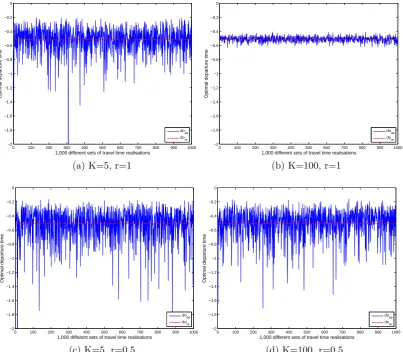
setting τ = 0. We generate 1,000 different sets of K travel time realisations and depict the optimal departure times in Figure 1. A comparison between Figures 1a and 1b highlights that limited storage capacity (K = 5 instead of K = 100) increases the variance of the optimal departure time considerably. This is a direct consequence of adaptive expectations being formed by a smaller number of travel time realisations. Figures 1c and 1d illustrate that for smaller values of r, the size of K becomes less relevant for the variance of optimal departure times. By definition, reducingrshifts attention towards more recent periods such that more distant travel time realisations have a negligible impact on the optimal departure time.

Transience has direct implications on the level of expected outcome utility as illustrated by Figure 2a. Even whenr→1, expected outcome utility falls belowEUreforK <∞, because

commuters have limited memory capacity to form rational expectations. A decrease in r results in a further deviation ofEUae fromEUrebecause more weight is given to more recent

periods. A similar insight is found for the VOR in Figure2b. Limited memory increases the value of reliability and the penalty is amplified for higher degrees of transience. Equations9 and18indeed confirm that the distance betweenV ORreandV ORaedecreases for increasing

K. The maximum distance between these two lines is in our case 1₂ γ12

(γ1−β1) =AC19.51 per hour

for K = 1. The latter results in a maximum VOR of AC32.22 per hour, which is about 2.5

times higher than the rational expectations outcome. Cantarella (2013) suggests values of 40-80% for the weight of the most recent experience in the expectation of the current traffic situations. When we assume r = 0.5 and K = 5, the most recent travel time experience determines about 50% of the travel time expectation and the value of travel time reliability isAC19.63, which is 45% higher than with rational expectations.

4.3. Accurate retrieval and anchored expectations

So far we have neglected the presence of an anchor. Equation 11 shows that commuters depart earlier when they have a higher anchor valueTA. Moreover, an increase inτ reduces

0 100 200 300 400 500 600 700 800 900 1000 −2

−1.8 −1.6 −1.4 −1.2 −1 −0.8 −0.6 −0.4 −0.2 0

1,000 different sets of travel time realisations

Optimal departure time

doae

dore

(a) K=5, r=1

0 100 200 300 400 500 600 700 800 900 1000 −2

−1.8 −1.6 −1.4 −1.2 −1 −0.8 −0.6 −0.4 −0.2 0

1,000 different sets of travel time realisations

Optimal departure time

doae

dore

(b) K=100, r=1

0 100 200 300 400 500 600 700 800 900 1000 −2

−1.8 −1.6 −1.4 −1.2 −1 −0.8 −0.6 −0.4 −0.2 0

1,000 different sets of travel time realisations

Optimal departure time

doae

dore

(c) K=5, r=0.5

0 100 200 300 400 500 600 700 800 900 1000 −2

−1.8 −1.6 −1.4 −1.2 −1 −0.8 −0.6 −0.4 −0.2 0

1,000 different sets of travel time realisations

Optimal departure time

doae

dore

(d) K=100, r=0.5

0 0.1 0.2 0.3 0.4 0.5 0.6 0.7 0.8 0.9 1 −14.5

−14 −13.5 −13

r

Expected Utility

Expected Utility ae: K=5 Expected Utility

ae: K=∞ Expected Utility

re

(a) Expected utility

0 0.1 0.2 0.3 0.4 0.5 0.6 0.7 0.8 0.9 1

12 14 16 18 20 22 24 26 28 30 32

r

Value of travel time reliability

Value of travel time reliability ae: K=5 Value of travel time reliability_ae: K=∞

Value of travel time reliability re

(b) Value of travel time reliability

definition reduces the variance in the latter measure. Naturally, the deviation between the anchor point and mean travel time defines whether optimal departure time coincides with rational expectations at τ = 1. The effects of the anchor point on expected utility and the value of travel time reliability are of more interest here. For this exercise we assume K = 5 and r= 1, resulting in ρk = _K1.

Figure3aillustrates that a quadratic penalty applies for deviations TA6=µwhenτ = 1.

For τ = 1 memory limitations do not play a role (since only the anchor counts), meaning that for a= 0 (i.e. when TA =µ) the expected utility is equal to the rational expectations

outcome. For values of τ between 0 and 1, however, an additional deviation from rational expectations due to the limited memory becomes present (even whena= 0). For this reason, the dotted horizontal line in Figure3afalls below the rational expectations utility level even when the anchor has no impact (τ = 0).11 _{Moreover the penalty for using a sub-optimal}

anchor point decreases for lower values ofτ. The latter is illustrated by the curve atτ = 0.5. Figure 3b plots the VOR as a function of τ. It follows directly from Equation 15 that the VOR reduces to the rational expectations outcome for τ = 1, since there is no penalty for forming adaptive expectations. Reducing the value of τ result in a larger effect of recent experiences on the formation of expectations, which increases the value of travel time reliability (see Figure2). In other words,τ controls the distance between the two horizontal lines in Figure2b. As expected, the effect is strongest for small values ofτ. The presence of an anchor point reduces the maximum deviation between the value of travel time reliability with rational expectations and adaptive expectations for any degree of transience.12

4.4. Inaccurate retrieval and transience

Finally, we illustrate the implications of inaccurate retrieval on expected utility, where we allow ¯ν to vary between zero and σ2 _{(see Equation 21). For plausibility, we set this upper}

bound on ¯ν such that deviations from actual realizations do not fall too much outside of the scale off(·). In accordance with Equation22, Figure4shows that the penalty for inaccurate retrieval is linear in ¯ν, where more inaccuracy reduces expected utility (but does not affect the VOR). This effect is further amplified for smaller values of r.

4.5. Summary of numerical results

We find that r and τ are the most important determinants of differences between adaptive and rational expectations in terms of optimal departure times and the value of travel time reliability. Based on Figure 2b we can conclude that the VOR may be underestimated by up to 45% if the VOR is computed under the assumption that the scheduling decisions are guided by rational expectations, whereas in reality they are guided by adaptive expectations and anchoring. We hereby interpretK = 5 andr = 0.5 as realistic lower boundaries for the memory storage capacity and the transience parameter, respectively (seeCantarella (2013)). Inaccuracy of retrievals leaves the VOR unaffected, but may induce additional dis-utility, although this effect seems to be relatively small (see Figure 4). The presence of an anchor

11_{For smaller values ofrthe distance between the two horizontal lines increases.} 12_{Whenτ is endogenously chosen, the VOR will depend onaandν}

−0.3 −0.2 −0.1 0 0.1 0.2 0.3 −16

−15.5 −15 −14.5 −14 −13.5 −13

a in hours

Expected Utility

Expected Utility_ae: τ=1 Expected Utilityae: τ=0, K=5, r=1

Expected Utility_ae: τ=0.5, K=5, r=1 Expected Utility_re

(a) Expected utility

0 0.1 0.2 0.3 0.4 0.5 0.6 0.7 0.8 0.9 1 12.5

13 13.5 14 14.5 15 15.5 16 16.5 17

τ

Value of travel time reliability

Value of travel time reliabilityae: K=5, r=1

Value of travel time reliabilityre

(b) Value of travel time reliability as a function of

τ (fora= 0)

Figure 3: Alternative values of a and τ

0 0.01 0.02 0.03 0.04 0.05 0.06

−14.5 −14 −13.5 −13

ν

Expected Utility

Expected Utility

ae: K=∞, r=0.5 Expected Utility

ae: K=∞, r=0.8 Expected Utility

re

(τ 6= 0) may under certain conditions increase the expected utility. When τ is exogenous, an increase inτ always decreases the bias in the VOR, which is in turn independent of the anchor itself.

5. Conclusions

We developed a model in which adaptive expectations are formed on the basis of past experi-ences and anchoring. Limited memory storage capacity, transience, inaccurate retrieval and anchoring result in sub-optimal decisions, and thereby translate into reductions in utility relative to the rational expectations outcome. We apply our model to scheduling choices of commuters during the morning commute, where travel times are stochastic. We show that the value of travel time reliability may be underestimated by up to 45% if rational expec-tations are assumed, while the true expectation formation process is adaptive. The benefits from reliability improvements thus tend to be significantly larger if travel time expectation formation is guided by limited memory, adaptive expectations and anchoring. Revealed pref-erence studies that use a reduced-form utility function probably already capture the biases formulated in this paper. Our results are therefore mainly important for stated preference analyses that ignore the process of expectation formation.

Our functional form assumptions on the utility function allowed us to derive a simple closed-form expression for the memory adjusted value of reliability. The analytical result has the potential to be incorporated in existing static transport network models. Equations 8 and 14 show that trip travel cost functions of the structure C =b1 +b2µ+b3µ2 +b4σ2 are

able to capture memory biases in an adequate way. Here, the parametersb1, b2, b3 andb4 are

functions of the underlying behavioural parameters related to scheduling (β0, β1 and γ1),

anchoring (τ and a), transience (ρ1, ..., ρK) and retrieval inaccuracy (ν1, ..., νK), and µ and

σ2 _{are functions of the number of travellers on the links that constitute the trip. For more}

general forms of the utility function this structure unfortunately breaks down and numerical analysis is needed.

Our dynamic memory model stands apart from static behavioural models where individ-uals treat probabilities in a non-rational way, since it predicts that commuters are sometimes optimistic and sometimes pessimistic, depending on their most recent experiences and cor-responding retrieval probabilities. This is in contrast to rank-dependent utility models that assume that optimism and pessimism are exogenously given and therefore unrelated to ear-lier experiences (see Koster and Verhoef (2012) and Xiao and Fukuda (2015) for transport applications).

Our approach may serve as an input for the modelling of dynamic systems, both in transport as well as in other fields of economics. In such models adaptive expectations often play a central role but are usually based on simple decision rules (see for example Watling and Cantarella(2013) for an overview of day-to-day dynamic transport systems andHommes (2013) for an overview of adaptive expectations in financial markets). Incorporating dynamic learning mechanisms in the model is a fruitful area for further investigation.

more general results. In the next paragraphs, several possible generalizations are discussed. First, we assume for simplicity that travel time distributions are independent of departure time, whereas in reality travel time distributions usually vary by time of day. In Appendix A we show how to generalize the resulting expressions for travel time distributions that are changing over subsequent days. This results in additional biases related to variations in travel time distributions over subsequent time periods.

Second, we assume that the decision-maker has a fixed anchor TA = µ+a, whereas

in reality this may well be a noisy belief, implying that a is random. The implications of randomness in the anchor can be discussed by looking at the impact on the variance and the mean departure time with adaptive expectations. Equation 12 then will include the mean anchor, whereas Equation 13 would have an additional variance term relating to the variation in the anchor. Because the variance of departure time will increase with a higher variance in the anchor, this will result in additional losses in expected utility (see Equation A.3).

Third, for the main analysis (except for Section 3.6, where we discuss the endogenous choice of the relative weight attached to the anchor, τ), we made the assumption that decision makers are not aware of their memory limitations (Piccione and Rubinstein,1997). For decisions where the stakes are not so high, this may be a reasonable assumption. When the utilitarian effects of sub-optimal choice are high, the decision maker may take a more reflective attitude and may optimise her anchor or collect additional information in order to reduce behavioural biases.

Fourth, we assumed that retrieval probabilities are independent of the values of the experienced states, meaning that negative experiences do not impact expectations more than positive ones, or vice versa. Furthermore, we assumed that the experience of a new state does not affect the memory of the already stored states. Future research should aim at relaxing these assumptions.

Further useful generalizations could be implemented with respect to the specification of the scheduling preferences as well as by including information. One might for instance employ more general scheduling preferences and then use Taylor approximations to arrive at more general results (see Engelson (2011)). It also seems a fruitful direction for future research to extend the model by the possibility to obtain information about future travel times. The quality of the information could then in turn depend on when the information is collected, or on how much one is willing to pay for it.

Bibliography

Arentze, T. A. and Timmermans, H. J. (2003). Modeling learning and adaptation processes in activity-travel choice a framework and numerical experiment. Transportation, 30(1):37–62.

Arentze, T. A. and Timmermans, H. J. (2005). Representing mental maps and cognitive learning in micro-simulation models of activity-travel choice dynamics. Transportation, 32(4):321–340.

Ariely, D., Loewenstein, G., and Prelec, D. (2003). ”Coherent arbitrariness”: Stable demand curves without stable preferences. The Quarterly Journal of Economics, 118(1):73–106.

Avineri, E. and Prashker, J. N. (2005). Sensitivity to travel time variability: Travelers learning perspective.

Transportation Research Part C: Emerging Technologies, 13(2):157–183.

Barucci, E. (1999). Heterogeneous beliefs and learning in forward looking economic models. Journal of

Evolutionary Economics, 9(4):453–464.

Barucci, E. (2000). Exponentially fading memory learning in forward-looking economic models. Journal of

Economic Dynamics and Control, 24(5):1027–1046.

Ben-Elia, E. and Shiftan, Y. (2010). Which road do I take? a learning-based model of route-choice behavior with real-time information. Transportation Research Part A: Policy and Practice, 44(4):249 – 264. B´enabou, R. and Tirole, J. (2002). Self-confidence and personal motivation. The Quarterly Journal of

Economics, 117(3):871–915.

Bernheim, D. B. and Thomadsen, R. (2005). Memory and anticipation. The Economic Journal, 115(503):271–304.

Bogers, E. A. I., Bierlaire, M., and Hoogendoorn, S. P. (2007). Modeling learning in route choice.

Trans-portation Research Record, 2014:1–8.

B¨orjesson, M., Eliasson, J., and Franklin, J. P. (2012). Valuations of travel time variability in scheduling versus mean–variance models. Transportation Research Part B: Methodological, 46(7):855 – 873.

Brunnermeier, M. K. and Parker, J. A. (2005). Optimal expectations. American Economic Review, 4(95):1092 – 1118.

Cantarella, G. E. (2013). Day-to-day dynamic models for intelligent transportation systems design and appraisal. Transportation Research Part C: Emerging Technologies, 29:117–130.

Caplin, A., Dean, M., and Martin, D. (2011). Search and satisficing. American Economic Review, 101(7):2899–2922.

Chen, R. and Mahmassani, H. (2004). Travel time perception and learning mechanisms in traffic networks.

Transportation Research Record, 1894(1):209–221.

Engelson, L. (2011). Properties of Expected Cost Function with Uncertain Travel Time. Transportation

Research Record, 2254:151–159.

Fosgerau, M. and Engelson, L. (2011). The value of travel time variance. Transportation Research Part B:

Methodological, 45(1):1–8.

Fosgerau, M. and Karlstr¨om, A. (2010). The value of reliability. Transportation Research Part B:

Method-ological, 44:38–49.

Fosgerau, M. and Lindsey, R. (2013). Trip-timing decisions with traffic incidents. Regional Science and

Urban Economics, 43(5):764–782.

Furnham, A. and Boo, H. C. (2011). A literature review of the anchoring effect. The Journal of

Socio-Economics, 40(1):35 – 42.

Gennaioli, N. and Shleifer, A. (2010). What comes to mind. The Quarterly Journal of Economics, 125(4):1399–1433.

Gollier, C. and Muermann, A. (2010). Optimal choice and beliefs with ex ante savoring and ex post disappointment. Management Science, 56(8):1272–1284.

Hensher, D. (2001). The valuation of commuter travel time savings for car drivers: evaluating alternative model specifications. Transportation, 28(2):101–118.

Hirshleifer, D. and Welch, I. (2002). An economic approach to the psychology of change: Amnesia, inertia, and impulsiveness. Journal of Economics & Management Strategy, 11(3):379–421.

Horowitz, J. L. (1984). The stability of stochastic equilibrium in a two-link transportation network.

Trans-portation Research Part B: Methodological, 18(1):13–28.

Jha, M., Madanat, S., and Peeta, S. (1998). Perception updating and day-to-day travel choice dynamics in traffic networks with information provision. Transportation Research Part C: Emerging Technologies, 6(3):189–212.

Koster, P. and Verhoef, E. T. (2012). A rank-dependent scheduling model. Journal of Transport Economics

and Policy, 46(1):123–138.

Mullainathan, S. (2002). A memory-based model of bounded rationality. The Quarterly Journal of

Eco-nomics, 117(3):735–774.

Noland, R. B. and Small, K. A. (1995). Travel-time Uncertainty, Departure Time Choice, and the Cost of Morning Commutes. Transportation Research Record, 1493:150–158.

Peer, S., Koopmans, C. C., and Verhoef, E. T. (2012). Prediction of travel time variability for cost-benefit analysis. Transportation Research Part A: Policy and Practice, 46(1):79–90.

Peer, S., Verhoef, E. T., Knockaert, J., Koster, P., and Tseng, Y.-Y. (2015). Long-run vs. short-run perspectives on consumer scheduling: Evidence from a revealed-preference experiment among peak-hour road commuters. International Economic Review, 56(1):303–323.

Piccione, M. and Rubinstein, A. (1997). On the interpretation of decision problems with imperfect recall.

Games and Economic Behavior, 20(1):3 – 24.

Sarafidis, Y. (2007). What Have you Done for me Lately? Release of Information and Strategic Manipulation of Memories. The Economic Journal, 117(518):307–326.

Schacter, D. L. (2002). The seven sins of memory: How the mind forgets and remembers. Houghton-Mifflin, New York.

Simon, H. A. (1955). A behavioral model of rational choice. The Quarterly Journal of Economics, 69(1):99– 118.

Small, K. A. (1982). The Scheduling of Consumer Activities : Work Trips.The American Economic Review, 72:467–479.

Small, K. A. (1992). Trip scheduling in urban transportation analysis. The American Economic Review, 82(2):482–486.

Strack, F. and Mussweiler, T. (1997). Explaining the enigmatic anchoring effect: Mechanisms of selective accessibility. Journal of Personality and Social Psychology, 73(3):437.

Tseng, Y.-Y. and Verhoef, E. T. (2008). Value of time by time of day: A stated-preference study.

Trans-portation Research Part B: Methodological, 42(7-8):607–618.

Tversky, A. and Kahneman, D. (1974). Judgment under uncertainty: Heuristics and biases. Science, 185(4157):1124–1131.

Vickrey, W. S. (1969). Congestion theory and transport investment.American Economic Review, 59(2):251– 260.

Vickrey, W. S. (1973). Pricing, metering, and efficiently using urban transportation facilities. Highway

Research Record, 476:36–48.

Watling, D. P. and Cantarella, G. E. (2013). Modelling sources of variation in transportation systems: theoretical foundations of day-to-day dynamic models. Transportmetrica B: Transport Dynamics, 1(1):3– 32.

Wilson, A. (2003). Bounded memory and biases in information processing. Econometrica, 6(82):2257–2294. Wilson, T. D., Houston, C. E., Etling, K. M., and Brekke, N. (1996). A new look at anchoring effects: basic

anchoring and its antecedents. Journal of Experimental Psychology: General, 125(4):387–402.

Xiao, Y. and Fukuda, D. (2015). On the cost of misperceived travel time variability.Transportation Research

Appendix A. Proof section 3.3.

In this Appendix we derive the predicted expected outcome utility (Equation14). The proof is for general travel distributions with k-dependent means and variances and k-dependent anchoring. Assume that travel time distributions have mean µk and variance σk2 and

prob-ability density f(Tk|µk, σk2). The predicted expected outcome utility is given by:

E_(Uae)≡E_(U(dae

0 , T0))

= Z ... Z Z ... Z

U(dae

0 , T0)

K Y

k=1

g T¯k|Tk, νk2

dT¯1...T¯K)

! _K

Y

k=0

f(Tk|µk, σk2)dT0...dTK,

(A.1)

The expectation over all values of T0 is given by:

E_T

0(U(d

ae

0 , T0)) =

Z

−

Z 0

dae

0

(β0+β1v)dv−

Z dae0 +T0

0

(β0+γ1v)dv !

f(T0|µ0, σ20)dT0

=−β0µ0−

1

2(γ1−β1)(d

ae

0 )2−γ1µ0dae0 −

1 2γ1(µ

2

0+σ02),

(A.2)

where we useE_T

0 to emphasize that the expectation is only over values ofT0. The predicted

expected outcome utility with adaptive expectation can be found by taking the expected value over all possible values of the departure time dae

0 :

E_{(Uae) =}E

−β0µ0−

1

2(γ1−β1)(d

ae

0 )2 −γ1µ0dae0 −

1 2γ1(µ

2 0+σ02)

=−β0µ0−

1

2(γ1−β1)E (d

ae

0 )2

−γ1µ0E(dae0 )−

1 2γ1(µ

2 0+σ02)

=−β0µ0−

1

2(γ1−β1) (E(d

ae

0 ))2+VAR(dae0 )

−γ1µ0E(dae0 )−

1 2γ1(µ

2

0+σ20).

(A.3) This shows that E_{(Uae) can be written as a function of the mean departure time and the}

variance of departure time. When travel time distributions depend onk, the departure time with adaptive expectations is given by11. The mean departure time is given by:

E_(dae

0 ) =−τ

γ1

γ1−β1

TA−(1−τ)

γ1

γ1−β1

K X

k=1

ρkµk, (A.4)

which reduces to12for µk =µ. The variance of the departure time is given by (here we use

the assumptions of footnote 6):

VAR_(dae

0 ) = (1−τ)2

γ1

γ1−β1

2 K

X

k=1

ρ2_k σ2_k+ν_k2

, (A.5)

which reduces to13, for σ2

k=σ2. Substituting EquationA.4 andA.5 in Equation A.3gives

assumeµk=µ0 =µand σk2 =σ02 =σ2 in order to arrive at the results that are discussed in

the main body of the paper. Substituting12 inA.3 gives:

E_{(Uae) =−β0µ−} 1

2(γ1−β1)

γ1

γ1−β1

2

µ2+ 2µτ a+τ2a2

+VAR_(dae

0 )

!

+ γ

2 1

γ1−β1

µ2+µτ a

− 1

2γ1(µ

2_+σ2₎

=−β0µ+

1 2

γ2 1

γ1−β1

−1

2γ1µ

2₋1

2γ1σ

2₋ 1

2 γ2

1

γ1−β1

τ2a2− 1

2(γ1−β1)VAR(d

ae

0 )

=−β0µ+

1 2

β1γ1

γ1−β1

µ2− 1

2γ1σ

2₋ 1

2 γ2

1

γ1−β1

τ2a2 −1

2(γ1−β1)VAR(d

ae

0 )

=E_(Ure)−1

2 γ2

1

γ1−β1

τ2a2−1

2(γ1−β1)VAR(d

ae

0 ).

(A.6) Substituting Equation13 gives the desired result. This concludes the proof.

Appendix B. Proof section 3.6.

We start with14 where we include the optimal anchor parameter τ∗

which depends on the variance of travel time (see 24). Then differentiate expected utility with respect to σ2 _to

obtain:

VORτ∗ =

1 2γ1+

1 2

γ2 1

γ1−β1

(1−τ∗

)2

K X

k=1

ρ2k+

γ2 1

γ1−β1

τ∗∂τ ∗

∂σ2a 2

− γ

2 1

γ1−β1

(1−τ∗

)∂τ

∗

∂σ2 σ 2

K X

k=1

ρ2k+ K X

k=1

ρ2kνk2 !

= 1 2γ1+

1 2

γ2 1

γ1−β1

(1−τ∗

)2 K X k=1 ρ2 k + γ 2 1

γ1−β1

τ∗∂τ ∗

∂σ2a

2_−(1−τ∗

)∂τ

∗

∂σ2 σ 2

K X

k=1

ρ2k+ K X

k=1

ρ2kνk2 !!

= 1 2γ1+

1 2

γ2 1

γ1−β1

(1−τ∗

)2

K X

k=1

ρ2k

+ γ

2 1

γ1−β1

∂τ∗

∂σ2 τ

∗

a2+σ2

K X

k=1

ρ2_k+

K X

k=1

ρ2_kν_k2

!

− σ2

K X

k=1

ρ2_k+

K X

k=1

ρ2_kν_k2

!!

= 1 2γ1+

1 2

γ2 1

γ1−β1

(1−τ∗

)2

K X

k=1

ρ2k,

Substituting24 gives:

VORτ∗ =

1 2γ1+

1 2

γ2 1

γ1−β1

a2

σ2PK k=1ρ2k+

PK

k=1ρ2kνk2+a2

!2 _K

X

k=1

ρ2_k

= 1 2γ1+

1 2

γ2 1

γ1−β1

a4PK k=1ρ2k

σ2PK

k=1ρ2k+

PK

k=1ρ2kνk2+a2

2,