Ab initio determination of coarse-grained interactions in double-stranded DNA

Ab initio determination of coarse-grained

interactions in double-stranded DNA

The Harvard community has made this

article openly available. Please share how

this access benefits you. Your story matters

Citation

Hsu, Chia Wei, Maria Fyta, Greg Lakatos, Simone Melchionna, and

Efthimios Kaxiras. 2012. “Ab Initio Determination of Coarse-Grained

Interactions in Double-Stranded DNA.” The Journal of Chemical

Physics 137 (10): 105102. https://doi.org/10.1063/1.4748105.

Citable link

http://nrs.harvard.edu/urn-3:HUL.InstRepos:41384025

Terms of Use

This article was downloaded from Harvard University’s DASH

repository, and is made available under the terms and conditions

applicable to Other Posted Material, as set forth at

http://

Ab initio

determination of coarse-grained interactions

in double-stranded DNA

Chia Wei Hsu,1_{Maria Fyta,}1,2_{Greg Lakatos,}1,3_{Simone Melchionna,}3,4

and Efthimios Kaxiras1,3,a)

1_{Department of Physics, Harvard University, Cambridge, Massachusetts 02138, USA} 2_{Department of Physics, Technical University of Munich, Garching 85748, Germany}

3_{School of Engineering and Applied Sciences, Harvard University, Cambridge, Massachusetts 02138, USA} 4_{IPCF-CNR, Istituto Processi Chimico-Fisici, Consiglio Nazionale delle Ricerche, Università La Sapienza,}

P.le A. Moro 2, 00185 Rome, Italy

(Received 12 December 2011; accepted 13 August 2012; published online 12 September 2012)

We derive the coarse-grained interactions between DNA nucleotides fromab initiototal-energy cal-culations based on density functional theory (DFT). The interactions take into account base and se-quence specificity, and are decomposed into physically distinct contributions that include hydrogen bonding, stacking interactions, backbone, and backbone-base interactions. The interaction energies of each contribution are calculated from DFT for a wide range of configurations and are fitted by simple analytical expressions for use in the coarse-grained model, which reduces each nucleotide into two sites. This model is not derived from experimental data, yet it successfully reproduces the stable B-DNA structure and gives good predictions for the persistence length. It may be used to re-alistically probe dynamics of DNA strands in various environments at theµs time scale and theµm length scale.© 2012 American Institute of Physics. [http://dx.doi.org/10.1063/1.4748105]

I. INTRODUCTION

Biological systems exhibit high degrees of complexity that are essential to the functions they perform. The DNA double helix is one such example: the properties of this macromolecule are directly influenced by its conformational variability as well as by environmental factors that include counterions, impurities, and temperature, as it performs a wide variety of vital cellular functions such as transcription and replication.1 _{A full account of such biological functions}

must rely on a realistic description of the physical processes that underlie them. Fine-grained calculations of DNA at the atomic level2,3 _{can provide this level of detailed description,}

but they are restricted to very small systems of order tens of base pairs and time scales of order ns, whereas most biologi-cal processes involve DNA behavior at the sbiologi-cale of more than a hundred base-pairs and take place at theµs time scale and beyond. To probe these biologically relevant processes, a real-istic and efficient coarse-grained model of DNA is necessary. Examples of crucial functions under current investigation that could benefit from a coarse-grained model of DNA include the translocation of DNA through nanopores4,5 _{in the}

con-text of ultra-fast electronic sequencing, DNA capture in and ejection from nanoscale capsules/wells, and the study of the interplay between histones and DNA during mitosis.6

The main theoretical challenge in biological systems is to bridge the scales between the atomistic and the macroscopic without wasting computational resources on uninteresting be-haviors, such as the internal dynamics within a base which practically never changes shape, or the motion of solvent molecules far from the biomolecule. Computational methods

a)_{Electronic mail: [email protected].}

of this type have been used before, for example, in the study of protein dynamics.7 _{Multiscale simulations have also been}

successfully applied to the study of the electronic behavior and electron localization in stretched dry DNA.8_{Our ultimate}

goal is to enable the study of variations in the DNA struc-ture using multiscale approaches that do not sacrifice accuracy while achieving high efficiency. In the present work we focus on the first stage toward this goal, namely, the development of a coarse-grained model capable of accurately reproducing the structure of double-stranded DNA (ds-DNA) in solution, and simple enough to be efficiently combined with multiscale simulation techniques.

Many coarse-grained models of DNA have been pro-posed in the past few years.9–21_{Most of them are constructed}

in a “top-down” fashion,9–17 _{where the interaction}

poten-tials are chosen to reproduce certain sets of experimental data. Bead-string models10 _{have been used to study}

diffu-sion and structural relaxation of single strands. Rigid base-pair models11 _{have been used to describe the elastic}

prop-erties of DNA.22,23 _{The three-site-per-nucleotide model by}

Knotts and coworkers14 _{captures the salt-dependent}

melt-ing of DNA, and has been extended to include solvent-induced attraction between DNA strands24 _{that helped to}

gain insights on hybridization25–27 _{and on certain}

sequence-dependent effects;28 _{this model has also been adapted to}

describe the mechanical denaturation of long DNA29 _and

to include explicit solvent molecules.30 _{Starr and}

cowork-ers proposed a simple model that captures the basics of hybridization,13 _{and this model has been used to study}

Holliday junctions31 _{and the self-assembly of DNA-linked}

nanoparticles.32 _{Ouldridge and coworkers proposed another}

model that is sequence independent, but can reproduce sev-eral structural, mechanical, and thermodynamic properties

DNA.16,33_{Another family of models starts from all-atom}

em-pirical force fields, and construct the coarse-grained model potentials from bottom-up.18–21 _{The model by Savelyev and}

coworkers18,34_{was parametrized by matching moments of}

ob-servables in the Hamiltonian. Other approaches to a bottom-up construction include minimizing difference between the all-atom and coarse-grained potentials,19_{imposing molecular}

bonding geometry constraints,20_{and inverting the Boltzmann}

function to get the coarse-grained potentials.21

Each of these models has its regime of validity, depend-ing on what experimental data were used for the model deriva-tion. In this work, we develop a minimal model of ds-DNA that incorporates sequence specificity and has realistic me-chanical robustness to bending and untwisting forces. We seek a model that is chemically accurate, yet not based on empiri-cal observations. For these purposes, we take a bottom-up ap-proach, and construct the potentials of the coarse-grained sys-tem directly from first-principles calculations. We divide the interaction potentials into independent parts that come from physically distinct contributions, and for each contribution we carry outab initiocalculations to find the functional forms of the potentials. We impose noa prioriassumption on the func-tional forms of the potentials—these are determined based on results of the ab initiocalculations. The present form of the model has its limitations that we will discuss, but it is flexible for future improvements.

This paper is organized as follows: in Sec.IIwe describe the methodology employed for the first-principles calcula-tions. In Sec.IIIwe present theab initiodata for each energy contribution and the analytical forms of the corresponding po-tentials. The implementation and performance of the coarse-grained model is described in Sec.IV. Finally, we present val-idations of the model in Sec.V, and conclude in Sec.VI.

II. METHODOLOGY OFAB INITIO CALCULATIONS

We carry out the first-principles calculations using den-sity functional theory (DFT).35 _{In our DFT calculations,}

we do not deal with environmental factors such as solvent molecules and ions, and the calculations are carried out at the ground state (zero temperature). The environment and tem-perature factors are addeda posterioriin the coarse-grained model through electric field screening and through Brownian dynamics. A more accurate approach will include tempera-ture dependence in the coarse-graining procedure, but this is a challenging task and is not yet taken into account in the cur-rent work. Presence of the water molecules and ions may also affect the energetics, but their effects are not investigated in this work.

We use SIESTA,36_{an electronic structure code based on}

atomic-like orbitals, to carry out the DFT calculations. This approach has been previously applied in similar studies of gas-phase DNA bases37 _{and successfully reproduces}

proper-ties such as optical response in comparison to available exper-imental data.38_{We use the Troullier-Martins scheme}39_to

ob-tain pseudopotentials to eliminate the core electrons from the calculation and to produce a smoother valence charge density. We use a basis of double-ζpolarized atomic orbitals for all the atoms involved (13 orbitals for C, N, O, and P; 5 orbitals for

H). An auxiliary real space grid equivalent to a plane-wave cutoff of 100 Ry is used for the calculation of the Hartree and exchange-correlation energies. For geometry optimization, a structure is considered fully relaxed when the magnitude of force on every atom is smaller than 0.04 eV/Å.

We use the generalized gradient approximation (GGA) with the PBE exchange-correlation functional40 _{to describe}

the backbone-base and the inter-base-pair interactions, as this functional is known to describe covalent and hydrogen bonds well.41,42 _{Interactions within the backbone are treated with}

the local-density approximation (LDA),43 _{which is adequate}

for describing small radial and angular deviations of covalent bonds from their equilibrium values. The interaction between stacked base-pairs has a large contribution from long-ranged van der Waals (vdW) forces and exhibits an elaborate energy landscape that depends sensitively on the geometry.44,45

Lo-cal or semi-loLo-cal exchange-correlation functionals cannot de-scribe such long-range effects:46 _{they do not reproduce the}

∼r−6 _{behavior at large separationrthat is characteristic of}

vdW interactions, and usually underestimate the stacking dis-tance between two planar structures. There exists empirical corrections that add the vdW effects to the energies obtained from DFT calculations,47_{but we find that such correction still}

leads to underestimation of the stacking distance. Therefore, we employ a non-empirical long-range vdW density func-tional developed by Dionet al.48_{to carry out calculations for}

the stacked base-pairs interactions.

The calculated interaction energy between two con-stituents may be susceptible to the basis set superposition error (BSSE), which results in unphysical lowering of the interaction energy when the two constituents come close to each other. To correct for BSSE, we take the full counterpoise approach:49 _{at each separationr, we optimize the dimer}

ge-ometry and carry out four additional calculations (constituent A along and constituent B along, with and without ghost or-bitals), and obtain the BSSE-corrected interaction energy as

E(r)₌EAB(r)−E′A(r)−EB′(r)+EA(r)+EB(r)

−EA∗−EB∗, (1)

where the subscript denotes the geometry: AB is the opti-mized dimer geometry, A and B are its constituent geometries, and A∗_{and B}∗_{are the individually optimized constituent} ge-ometries; the prime indicates that ghost orbitals of the other constituent are used in the energy calculation.

III. CONSTRUCTION OF MODEL POTENTIALS

base (1)

(2)

T

A

(1)

(2)

base

sugar sugar

r

(a)

H1

H9

CN

r

φ

CC

r

(b)

hb

φhb

r

N9

C1

C1

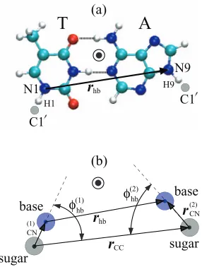
FIG. 1. Schematic of an adenine-thymine (AT) base-pair showing the geo-metric variables in the hydrogen bond potential in (a) the atomic structure calculations and (b) the coarse-grained model. The distancerhb, the two flip-anglesφ(_hbi), and the dihedral angleθd(angle between the two base planes, not shown) are used to describe interaction between the two bases. The vectors

rCCandr(CNi) are used to define the normal vectors of the two bases and the dihedral angle. In this figure and Figs.4and7, the colored spheres represent C (cyan), H (white), N (blue), O (red), and P (brown) atoms.

facilitates direct comparison to experimental structures dur-ing validation of the model.

To derive the effective interaction between these coarse-grained sites, we follow earlier work50 _{and decompose the}

total interaction energy into contributions that have distinct physical meanings: the hydrogen bond between complemen-tary basesEhb, the stacking energy between neighboring

base-pairs Est, contributions from the backboneEbb, and

electro-static interaction between the charged phosphate groupsEel:

Etotal=Ehb+Est+Ebb+Eel. (2)

These are physically distinct contributions, and in our model they are treated as independent and additive. Each contribu-tion depends on several variables, and the effect of these vari-ables are not taken as independent.

The choice of the coarse-grained sites and the decompo-sition of the interaction potentials has determined the struc-ture of the model. The remaining construction of the model is to find explicit functional forms for each contribution, which we address in the following.

A. Hydrogen bonding

We consider first the interaction between two comple-mentary bases: adenine-thymine (AT) or guanine-cytosine (GC), which comes from hydrogen bonds. We consider its dependence on the base-to-base separation and on the rela-tive angles between the planes of the two bases. The angular dependence keeps the two bases coplanar and maintains the correct base-pair geometry.

We calculate the interaction energy as a function of the distancerhbbetween the pyrimidine N1 atom and the purine

N9 atom (see Fig.1), by starting from the energy-minimized

8 9 10 11 12

rhb (Å) -1

-0.5 0 0.5 1 1.5

Ehb_r

(eV) 0 30 _θ 60 90 120

d (deg) -1

-0.5 0

Ehb_d

(eV)

AT

GC

AT

GC

FIG. 2. Hydrogen bonding energy versus distancerhbbetween two compli-mentary bases. Inset shows the dependence on the dihedral angleθdbetween the two bases. Symbols are BSSE-corrected results from DFT calculations, and lines are fittings to Eqs.(3)and(4)with parameters given in TableI.

geometry and varyingrhbby translating the two bases parallel

to the direction of the hydrogen bonds. At eachrhbvalue, we

optimize the geometry while fixing the four atoms that cor-respond to the coarse-grained sites (N1 and H1 of the pyrim-idine, and N9 and H9 of the purine) to preserve rhb and the

relative angles. At smallrhb values, the atoms are also

con-strained on the base-pair plane to prevent the two bases from rotating out of plane. The effect of flipping angles and of non-planarity will be examined separately.

Figure2shows the calculated interaction energy, which can be described by the universal binding energy relation (UBER)51

Ehb_r(rhb)=E0(1+a∗)e−a∗, a∗=(rhb−r0)/ l, (3)

with its minimum atrhb=r0,Ehb_r=E0. The parametersE0,

r0, andlare given in TableI. The energy at the minimum is

−0.64 eV for AT and₋1.17 eV for GC, in agreement with the values₋0.60 eV and₋1.17 eV, respectively, obtained in pre-vious calculations of the DNA hydrogen bonds.42_{We do not}

parametrize the base-to-base interaction between mismatched base-pairs, but doing so will be a straightforward extension of the current work.

Next we examine the effect of non-planarity of the bases: when the two planes of the bases are not aligned, the hydrogen bond weakens. We measure non-planarity by the dihedral an-gleθdbetween the planes of the two bases. Starting from the

energy-minimized geometry (θd=0), we varyθdby rotating

the two bases in opposite directions around the line from the pyrimidine N1 atom to the purine N9 atom. To keepθdfixed,

we optimize the geometry while holding the 6-fold ring of the

TABLE I. Fitting parameters for the radial dependence of the hydrogen bond interaction in Eq.(3)and the dihedral angle dependence in Eq.(4).

bp E0(eV) r0(Å) l(Å) kd

TABLE II. Fitting parameters for the flip-angle interaction in Eqs.(6)and (7), and the backbone base-sugar-sugar angle potential in Eq.(18).kbssis in 10−4_eV/deg2_{, all angles are in degrees.}

Base φ_hb(i,0) σ(i) kbss θ₃(0)′ θ5(0)′

A 54.53 18.67 3.489 94.17 61.36 T 55.93 16.82 4.689 92.67 68.40 G 52.69 25.57 4.165 90.30 63.69 C 54.87 22.43 6.178 91.55 66.37

two bases fixed. The resulting energies are shown in the inset of Fig.2. We fit the interaction energy with the expression

Ehb_d(θd)=E0ekd(cosθd−1), (4)

whereE0is the same as in Eq.(3); values of the parameterkd

are given in TableI.

The interaction between the two bases also depends on the in-plane angles of the two bases. In our coarse-grained model, this is described by the flip-angleφ_hb(i)for the two bases (i₌1, 2), defined as the base1-sugar1-sugar2 angle fori₌1 and the base2-sugar2-sugar1 angle for i₌2 (see Fig.1(b)). The flip-angles in the ground-state configuration, φ_hb(i,0), are listed in TableII. Starting from the energy-minimized geom-etry (φ(i)

hb =φhb(i,0)), we consider either rotating the pyrimidine

around the H1 atom, or rotating the purine around the H9 atom. The anchoring hydrogen atom mimics the backbone, which in physiological conditions remains relatively station-ary when base flipping occurs. To keepφ_hb(i) fixed at each ro-tated configuration, we optimize the geometry while fixing the pyrimidine atoms N1 and H1, and the purine atoms N9 and H9. For rotation inward, the atoms are constrained on the base-pair plane to prevent the two bases from rotating out of plane.

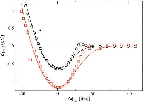
The resulting energies are plotted as a function of %φ_hb(i) ₌φ_hb(i)₋φ_hb(i,0)in Fig.3. When%φ_hb(i)is positive, the en-ergy is attractive and decays to zero. When%φ_hb(i)is negative, the two bases repel each other. We describe these two types of behavior separately, and fit the base-flipping interaction

en--50 0 50 100

∆φhb (deg) -1

-0.5 0 0.5 1

Ehb_f

(eV)

A

G

FIG. 3. Hydrogen bonding energy versus flip-angleφhbof A and G (results for T and C are similar and are not shown). Symbols are BSSE-corrected results from DFT calculations, and lines are fitting to Eq.(5)with parameters given in TableII.

ergy to the expression

E_hb(i)_{_f}!φ_hb(i)"₌E_hb(a,i_{_})_f!%φ_hb(i)"₊E_hb(b,i_{_})_f!%φ_hb(i)" (i₌1,2), (5) where E_hb(a,i_{_})_f is described by an exponential andE_hb(b,i_{_})_f is de-scribed by a harmonic spring

E_hb(a,i_{_})_{f =}E0

# exp

$

−

! %φ_hb(i)"2

2σ2

%

&!%φ_hb(i)"₊&!₋%φ_hb(i)" &

, (6)

E_hb(b,i_{_})_{f =}E0

$

−

! %φ_hb(i)"2

2σ2

%

&!₋%φ_hb(i)", (7)

and&is the step function. Again,E0is the same as in Eq.(3).

The values of the parameterσare listed in TableII.

Up to this point we have the interaction potential be-tween the two complementary bases as a function ofrhb,θd,

φ_hb(1), andφ_hb(2)individually while keeping other variables fixed at the equilibrium values. Here we assume that the interac-tion depends only on these four variables; even in this case, the general dependence is not trivial, as the four variables are not independent. For example, whenθdor%φ(hbi)is large,

the hydrogen bond is basically broken, and there should no longer be a strong dependence on rhb. To capture the

inter-dependences between the variables while keeping a reason-ably simple form for the interaction, we define the following functions

τhb_d(θd)=Ehb_d(θd)/E0,

τ_hb(i)_{_f}!φ_hb(i)"₌E_hb(a,i_{_})_f!%φ_hb(i)"/E0 (i=1,2) (8)

and take the final expression of the hydrogen bonding energy to be

Ehb!rhb,θd,φhb(1),φ(2)hb

"

=Ehb_r(rhb)τhb_d(θd) 2

'

i₌1

τ_hb(i)_{_f}!φ_hb(i)"

+

2

(

i₌1

E_hb(b,i_{_})_f!φ_hb(i)". (9)

Note that the repulsive part of the flipping interaction E_hb(b,i_{_})_f is treated as additive since it does not serve to weaken the bond; this also ensures that the modulation functions τ_hb(i)_{_f} take values strictly between 0 and 1. Equation(9)is reduced to Eqs.(3)–(5)for close-to-minimum geometries, i.e.,

Ehb!rhb,0,φhb(1,0),φ(2hb,0)

"

=Ehb_r(rhb), (10a)

Ehb!r0,θd,φhb(1,0),φ(2hb,0)

"

=Ehb_d(θd), (10b)

Ehb!r0,0,φ(1)hb,φhb(2,0)

"

=Eflip!φhb(1)

"

. (10c)

d

1

d

1

d

2

d

2

tw

(b)

θ

(a)

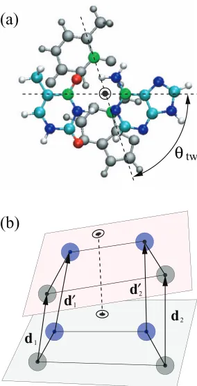
FIG. 4. Schematic showing two stacked base-pairs in (a) the atomic structure calculation (top view), and (b) the coarse-grained model (side view). In (a), the bottom base-pair is shown in gray for clarity. The atoms used to define the twist angleθtware colored in green, and the axis of the double helix (shown as a dotted circle) is defined as the 1:2 weighted center of the green atoms. In (b), the planes of the two base-pairs are shown. The twist angle is reduced for clarity of illustration. The four vectorsd1,d′

1,d2, andd′2as indicated are used to define the stacking distancerstin the coarse grained representation. See main text for description of the other geometric variables involved in stacking.

B. Stacking interactions

We turn next to the interaction between two stacked base-pairs. We consider the dependence on the stacking distance rstbetween the two base-pairs first. The two base-pairs are

re-laxed and stacked in parallel. Following usual conventions,1

we define the axial point of each base-pair to be the 1:2 weighted center of the pyrimidine C4 atom and the purine C6 atom, and define the twist angleθtwto be the angle made

by the C4–C6 vector of the two base-pairs. This is illustrated in Fig.4(a). The two base-pairs are stacked so that their axial points align at a distancerst apart in the direction normal to

the base-pair plane, and so that the twist angleθ_twis 36◦. The precise definition ofrst andθtw in the coarse-grained model

will be described in the Sec.IV.

There are ten different combinations of stacking, known as the ten Watson-Crick nearest-neighbors. For each of these ten combinations, we vary rst from 2.5 Å to 5.0 Å and

cal-culate the interaction energy without further relaxation. The results are shown in Fig. 5. At this range of rst, the energy

variation is well described by the expression

Est_r(rst)=−ϵ

# 5

) rm rst

*6

−6 )

rm rst

*5&

, (11)

3 4 5

r_st (Å)

-1 0 1 2 3 4

Est_r

(eV)

AT-AT

GC-GC

GC-AT

AT-TA

GC-CG GC-TA

FIG. 5. Stacking energy between two neighboring base-pairs (results for AT-GC, CG-AT-GC, TA-AT-GC, and TA-AT stacking are similar and are not shown). Symbols are BSSE-corrected results from DFT calculations using vdW den-sity functionals, and lines are fitting to Eq.(11)with parameters given in TableIII. For clarity, curves are shifted upward by increments of 0.6 eV; the curve for AT-AT stacking is not shifted. In our notation, GC-AT indicates the stacking of GC base-pair and AT base-pair with GA and TC following the 3′_–5′_direction.

which has a minimum at rst =rm, Est_r=ϵ. The resulting

values of the parameters from fitting theab initiovalues with this expression are listed in TableIII. It may seem surprising that the attractive part of the interaction behaves asr_st−5. This is no coincidence: the attraction between the two base-pairs is due to the vdW force, which behaves asr−6_{for two point}

particles and asr−4_{for two thin sheets (assuming additivity of}

the vdW interaction). The range ofr_stbeing considered here is comparable to the radius of the base-pairs (about 4 Å), so we expect a power in between the two, i.e.,r_st−5. We find this is indeed the case; expressions with any other integer power of rst lead to poor fitting. Again, we do not parametrize the

stacking interaction for mismatched base-pairs, which can be a straightforward extension to the current work.

Another dependence of the stacking interaction comes from the twist angle θtw. To examine this dependence, we

fixrstat 3.4 Å and varyθtw from 0◦to 360◦. Again, the two

base-pairs are parallel and have their axial points aligned. The

TABLE III. Fitting parameters of the stacking interaction in Eq.(11)for the ten Watson-Crick nearest-neighbors. In our notation, GC-AT indicates the stacking of GC base-pair and AT base-pair with GA and TC following the 3′_–5′_direction.

bps rm(Å) ε(eV)

AT-AT 3.550 −0.567

GC-GC 3.580 ₋0.477

GC-AT 3.566 −0.555

AT-TA 3.546 ₋0.530

GC-CG 3.498 −0.632

GC-TA 3.543 −0.549

AT-GC 3.535 −0.538

CG-GC 3.537 −0.563

TA-GC 3.613 −0.529

0 120 240 360 θtw (deg)

-0.4 0 0.4 0.8 1.2

Etw

(eV)

AT-AT

GC-GC

GC-AT

AT-TA

GC-CG GC-TA

FIG. 6. Twisting energy between two neighboring base-pairs. Symbols are BSSE-corrected results from DFT calculations using vdW density function-als, and lines are fitting to Eq.(12)with parameters given in TableIV. For clarity, curves are shifted upward by increments of 0.3 eV; the curve for AT-AT stacking is not shifted. Notation is same as in Fig.5. Note that, although there are 10 unique stacking combinations, only 6 are necessary in the eval-uation ofEtw. For example,Etw(θtw) of AT-GC is given byEtw(360◦−θtw) of GC-AT.

resulting energies Etware shown in Fig.6. This energy term

has a complex dependence onθtw, defying a simple

analyti-cal expression. Given its periodicity, we fitEtwwith a Fourier

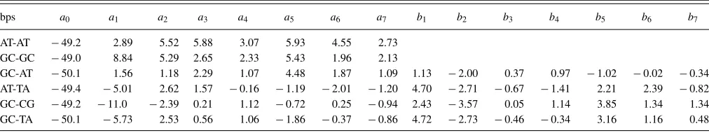
series:

Etw(θtw)=a0+ 7

(

n₌1

[ancos(nθtw)+bnsin(nθtw)]. (12)

The resulting values of the coefficients in this expansion are given in Table IV. For AT-AT and GC-GC stacking, Etw(−θtw)=Etw(θtw) by symmetry, and so the coefficients

bn are zero. We note that although Eq. (12)involves many trigonometric functions, the higher terms can be obtained from trigonometric addition rules or from the Chebyshev method. Therefore, its computational cost is similar to that of Eq.(11).

The stacking interaction also depends on the tilt-angleθtl,

which we define as the angle between the normal vectors of the two base-pair planes. The two base-pairs can tilt in a vari-ety of ways, and so this dependence can be complex. We find that close to the optimal stacked configuration (at smallθtl,

andrst=rm,θtw =36◦), the interaction energy dependence

can be approximately described by

Etl(θtl)=ϵcos2(θtl), (13)

where εis the same as in Eq.(11). This expression also has the physical meaning that the energy is at a minimum in the case of parallel (θtl=0) and anti-parallel (θtl=π) stacking,

and is zero when the two base-pairs are perpendicular to each other (θtl= ±π/2).

The interaction between two stacked base-pairs depends onrst,θtw, andθtl. To capture all three dependences and their

correlations with a reasonably simple form, we define the fol-lowing functions:

τtw(θtw)=Etw(θtw)/ϵ, τtl(θtl)=Etl(θtl)/ϵ (14)

and take the final expression of the stacking interaction to be

Est(rst,θtw,θtl)=Est_r(rst)τtw(θtw)τtl(θtl), (15)

similar to our treatment of the hydrogen bond. Equation(15)

involves much simplification, as the true interaction energy may depend on more than these three variables, and the dependence on rst, θtw, and θtl may not factorize. By the

same argument as for the hydrogen bonds, though, we expect Eq.(15)to be a good approximation close to equilibrium.

The stacking potential here is formulated as interaction between neighboring base-pairs, rather than between neigh-boring bases. This approach is sufficient when dealing with ds-DNA structures. However, we note that it may not be appropriate in processes like melting or hybridization that involve single-stranded DNA or broken base-pairs. In such situations, the stacking interaction should be reformulated as interaction between bases instead and be constructed in a similar fashion.

C. Backbone contribution

We next consider contributions from the backbone. First, to extract interactions within the sugar-phosphate backbone as distinct from any electrostatic or stacking interactions, we take the phosphate groups to be protonated and carry no charge, and replace the bases with terminating hydrogens. Starting from the energy-minimized geometry, we uniformly stretch or compress the backbone along the helical direction, as illustrated in Fig. 7(a), and allow the phosphate units to relax. The resulting energyEbb_ris shown in Fig.8as a

func-tion ofr_ss, the distance between the C1′_{atoms of neighboring} sugars. The interaction energy per sugar-phosphate unit can be described by the expression

Ebb_r(rss)=c2(rss−rss_0)2+c4(rss−rss_0)4 (16)

with c2 = 18.773 eV/Å2, c4 = 0.333 eV/Å4, and rss_0

=4.976 Å.

TABLE IV. Fitting parameters of the twisting interaction in Eq.(12). All parameters in units of 0.01 eV. Notation is same as in TableIII.

bps a0 a1 a2 a3 a4 a5 a6 a7 b1 b2 b3 b4 b5 b6 b7

AT-AT −49.2 2.89 5.52 5.88 3.07 5.93 4.55 2.73 GC-GC −49.0 8.84 5.29 2.65 2.33 5.43 1.96 2.13

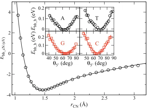
FIG. 7. (a) A single backbone strand in its relaxed B-DNA form, used to evaluate the backbone interactionEbb_r. The variablerssis the distance be-tween the C1′atoms of neighboring sugars, and is shown in the magnified part. (b) Structure used to evaluate the base-sugar-sugar interactionEbb_b. The vectors used to define the anglesθ3′andθ5′are shown.

The base is covalently bonded to the backbone. For this interaction, we consider only a base and a sugar, with the phosphate groups replaced by hydrogen atoms. Starting from the energy-minimized geometry, we translate the base and the sugar groups in opposite directions along the vector connect-ing the two. Then we hold the two atoms of the base-sugar covalent bond fixed, optimize the geometry, and calculate the interaction energy. We find results for the four bases to be nearly identical, so only results for guanine will be discussed. These are shown in Fig.9, with a fit to the UBER expression that includes two additional terms

Ebb_c(rCN)=E0(1+a∗+f2a∗2+f3a∗3)e−a∗,

a∗₌(rCN−r0)/ l, (17)

where rCN is the distance between the sugar C1′ atom and

the base N atoms (N9 of purines or N1 of pyrimidines). The values of the parameters are:E0=−3.542 eV,r0=1.455 Å,

l₌0.400 Å,f2=−0.132, andf3=0.215.

The base also interacts with neighboring backbone groups, and this gives rise to the 5′_/3′ _{asymmetry of the} double-helix. We characterize this interaction using the

an-4.6 4.8 5 5.2 5.4

r_ss (Å)

0 2 4 6

Ebb_r

(eV)

FIG. 8. Backbone energy per sugar-phosphate unit as a function of rss, the distance between adjacent C1′ _{atoms of the sugars. Solid line is fitting}

to Eq.(16).

0 0.1 0.2

Ebb_b

(eV)

40 50 60 70 80 θ5’ (deg) 0

0.1 0.2

Ebb_b

(eV)

50 60 70 80 90 θ5’ (deg)

1 1.5 2 2.5 3

r_CN (Å)

-4 -2 0 2 4

Ebb_cN

(eV)

A T

G C

FIG. 9. Interaction energy between the backbone and the base. Main plot shows the covalent bond energy between the sugar and the base, as a function of the distance between the sugar C1′_{atom and the base N1 or N9 atom to}

which it is bonded; solid line is fitting to Eq.(17). Inset shows the energy as a function of the sugar-sugar-base angleθ5′defined in Fig.7(b), and lines are fits to Eq.(18)with parameters given in TableII.

gle between the backbone strand and the base. We consider a segment of single-stranded DNA, with three sugar groups connected by two protonated phosphate groups. The first and third bases are replaced with terminating hydrogen atoms, and the middle base is either A, C, G, or T (see Fig. 7(b)). From the energy-minimized geometry, we rotate the mid-dle base around the vector rCC5′×r_CN (both are shown in Fig.7(b)), with the pivot point at C1′_{of the middle sugar. For} each rotated configuration, we relax the system while hold-ing the connecthold-ing N atom of the base (N9 of purines or N1 of pyrimidines) and the C1′_{atoms of the three sugars fixed.} The resulting energy is shown in the inset of Fig.9. We con-sider this energy to be a function of the two anglesθ3′andθ5′, whereθ3′is the angle betweenrCNandrCC3′, andθ5′is the an-gle betweenrCNandrCC5′ (see Fig.7(b)). We fit this energy term with the function

Ebb_b=

kbss

2 +!

θ3′−θ₃(0)′ "2

+!θ5′−θ₅(0)′ "2,

, (18)

where θ₃(0)′ and θ₅(0)′ are the angles in the initial configura-tion relaxed without constraint, andk_bssis obtained from fit-ting. The resulting values for these parameters are listed in TableII.

We treat Eqs.(16)–(18)as independent interactions, and so the total contribution of the backbone and its interaction with the base-pairs is given by

Ebb =Ebb_r+Ebb_c+Ebb_b. (19)

D. Electrostatics

physiological conditions, DNA is solvated in an aqueous elec-trolyte, and the phosphate groups in DNA are deprotonated. Therefore, we place a charge of−eon each sugar-phosphate group of the coarse grained model, and include a Coulomb potential between these groups

Eel(r)= e

2

4π ε0ε(r)r (20)

with a distance-dependent dielectric functionε(r),rbeing the distance between the charges andε0the dielectric constant in

vacuum. Thisε(r) plays two roles: (i) it incorporates the ef-fects of ionic screening, and (ii) it accounts for the fact that closely spaced interacting groups are only partially solvated by the surrounding electrolyte. We use the following expres-sion, closely related to the formulation of Ref.52, for the di-electric function:

ε(r)=

⎧ ⎪ ⎪ ⎨ ⎪ ⎪ ⎩

εint, forr < r0

εinteα(r−r0), forr0< r < r1

ε_∞eκr, forr > r1

, (21)

whereε_∞=78 is the dielectric constant of water, andεint is

the dielectric constant in theinteriorof the DNA helix, which we take to be 3.52_{The Debye length isκ}−1_{, related to the ionic}

strengthIthrough

κ−1₌ 1

ε0ε∞kBT

2NAe2I

, (22)

wherekBTis the thermal energy andNA is Avogadro’s num-ber. For example, at [Na+_{] = 0.1 M, the Debye length is} 9.6 Å. The valuesr0andr1 determine the boundary between

unscreened and screened electrostatic interactions. The char-acteristic sizes of the chemical groups represented by our coarse-grained units range from about 2 Å to about 5 Å. Con-sequently we setr0 =4 Å. Similarly, we chooser1=13 Å,

approximately five times the mean water oxygen–water oxy-gen distance in bulk water,53 _{as the distance where the}

ef-fective dielectric constant recovers the value predicted from the Debye-Hückel theory of screening in a bulk electrolyte. The value of αis then chosen such thatε(r) is continuous. Between the two charged groups within the same base-pair, ε(r)=ε_∞is used. Finally, since the electrostatic interaction decays exponentially at large distance, we truncate this inter-action for distances above five times the Debye length. The simple electrostatics approach here is a first approximation, and is not meant to capture details such as the dependence of ion condensation on conformation,54 _{which will require}

ex-plicit solvent molecules.

IV. IMPLEMENTATION AND PERFORMANCE OF THE COARSE-GRAINED MODEL

In Sec.IIIwe derived the interactions between the coarse-grained sites. The total interaction energy is given by Eq.(2), and the different contributions include summations over all relevant interacting units. Specifically,Ehbincludes a

summa-tion over all base-pairs, and Est includes a summation over

all pairs of neighboring base-pairs. Of the three terms that comprise the Ebb contribution, Ebb_r includes a summation

over all pairs of neighboring backbone sites, Ebb_c includes

a summation over all pairs of connected backbone and base sites, and Ebb_b includes a summation over all bases.

Fi-nally, Eel includes a summation over all pairs of backbone

sites.

Next, we relate the geometrical variables to the positions of the coarse-grained sites. In the coarse-grained representa-tion, the base site is identified with be the pyrimidine N1 atom or the purine N9 atom, and the backbone site is identified with the sugar C1′_{atom. Then the distance and angle variablesrhb,} φ_hb(1),φ_hb(2),rss,rCN,θ3′, andθ5′ follow from the position of the coarse-grained sites. We define the remaining geometrical variables as follows. For each base-pair, we define the normal vector of base ito ben(i)_=r

CC×r(CNi) withi=1, 2

corre-sponding to the two bases, and withrCC andr(CNi) defined in

Fig.1(b). The dihedral angleθdof this base-pair is given by

cosθd =nˆ(1)·nˆ(2), with the hat denoting unit vectors. We

de-fine the average normal of this base-pair to ben₌n(1)_+n(2)_,

and let the tilt-angle θtl between base-pair j and base-pair

j ₊ 1 be given by cosθtl=njˆ ·njˆ +1. As for the stacking

distancerst, we take the average distance of the four sites in

base-pair j₊1 to the plane of base-pair j. Specifically, we compute the four vectorsd1,d′1,d2, andd′2shown in Fig.4(b),

project them onto the two normal vectors aszi =di·nˆ(i)and

z′_{i =}d′_i·nˆ(i) for i ₌ 1, 2, and take rst=(z1

+z′₁₊z2+z′2)/4. Finally, the twist angle θtw is defined as

the angle between rCC,j and rCC,j₊1−(rCC,j₊1·nˆ(1)j )ˆn

(1)

j , which is the projection of rCC,j+1 onto the plane of

base-pairj.

We implement this model for calculations in the micro-canonical ensemble (constant number of particlesN, volume V, and energy E) and the canonical ensemble (constant N, V, and temperature T) with implicit solvent Brownian dy-namics. We choose the mass of each site to be the total mass of the group of atoms that it represents: 178 amu for the backbone site, 134 amu for base A, 125 amu for T, 150 amu for G, and 110 amu for C. Multiple-time-step integra-tors are used for time propagation: the RESPA algorithm55

is used for the N V E ensemble, and the multiple-time-step stochastic integrator56 _{is used for Brownian dynamics. The}

Coulomb interaction between different base-pairs is treated as the slow-varying component of the Hamiltonian, integrated with a time-step of 20 fs, while all the other forces are categorized into the fast-varying component of the Hamil-tonian, integrated with a time-step of 6.67 fs (i.e., three divisions per large time-step). This choice of time-steps en-sures high stability: when running in theN V E ensemble at 300 K, the total energy is conserved to within 5 _×10−4 _eV

per base-pair for arbitrary sequences at several conditions tested.

of base pairs, since the electrostatic interactions are damped. This performance makes simulations of ds-DNA in the µm length scale andµs time scale feasible.

V. MODEL VALIDATION

The different contributions in the model potentials have been derived from calculations of isolated units. Here we test the validity of the combined potential (additivity of the indi-vidual contributions), and its performance in larger systems (transferability of the potentials). Also, oura posteriori inclu-sions of the ionic and temperature effects are crude, and their consequences will also be assessed.

A. Equilibrium structure

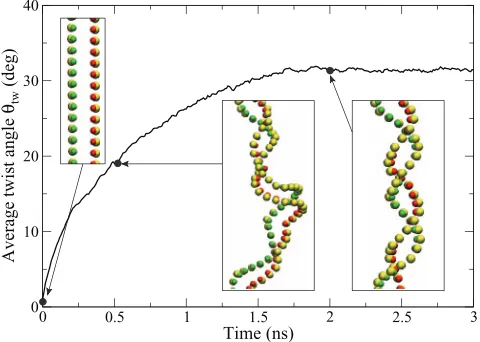
First, we test the structure prediction of the model with poly-AT DNA consisting of 250 base-pairs (bp) at temper-ature 300 K and salt concentration 0.1 M. When initialized with coordinates of the B-form DNA,57 _{the B-DNA}

struc-ture is maintained. To test the robustness of our model po-tential, we also carried out simulations starting with a highly off-equilibrium structure—an elongated and uncoiled double strand—and followed the evolution. Figure 10shows that in such case, the system is able to coil back to the B-DNA struc-ture. Signatures of the B-DNA structure such as the major groove, minor groove, and the 10 bps-per-turn period are well reproduced. This demonstrates the model’s ability to predict the stable double helix structure, without resorting to Go-like potentials that are defined relative to a specific reference struc-ture as in Ref.14.

To be quantitative, we calculate the averages of many structural properties after the system equilibrates. These quantities are listed in TableV, with comparison to reference values derived from recent crystallographic data of a natu-rally occurring 16 bps oligomer.58 _{The average deviation of}

our model from experiment is about 2%. Given that no

exper-0 0.5 1 1.5 2 2.5 3

Time (ns)

0 10 20 30 40

Average twist angle

θtw

(deg)

FIG. 10. Coiling of a 250-bp poly-AT strand in the coarse-grained model. The system starts in a completely uncoiled state and evolves at temperature 300 K. Insets show the middle part of the strand at time 0 ns, 0.5 ns, and 2.0 ns. Backbone sites are in yellow, A’s in red, and T’s in green.

TABLE V. Average structural properties of a 250 base-pair poly-AT strand at 300 K and salt concentration 0.1 M. The reference experimental values are derived from the positions of the C1′_{atoms of the sugars, the N1 atoms}

of the pyrimidines, and the N9 atoms of the purines in the crystal structure of Ref.58.

Difference Quantity Simulation Experiment58 _{(% )}

H bond distance rhb(Å) 8.96 8.93 0.3 Stacking distance rst(Å) 3.68 3.54 3.9 Backbone distance rss(Å) 4.99 4.91 1.5 Sugar-base distance rCN(Å) 1.46 1.47 0.5 Flip-angle φhb 54.1◦ 55.6◦ 2.7 Twist-angle θtw 31.4◦ 33.5◦ 6.2 Tilt-angle θtl 7.81◦ 8.00◦ 2.4 Backbone angle θ3′ 96.5◦ 94.3◦ 2.3 Backbone angle θ5′ 62.3◦ 63.2◦ 1.5

imental data were used in the model construction, this close agreement with experiment is remarkable.

B. Persistence length

Next, we check the model’s ability to predict mechanical properties at long lengths by examining the persistence length (lp), which gives an estimate of the bending rigidity of DNA.

The persistence length can be extracted from the decay of the orientational correlation function

⟨rˆi·rˆj⟩=e−sij/ lp, (23) where ˆriis the unit tangent vector at base-pairi, andsijis the arc length from base-pairito base-pairj. The tangent vectors and the arc length are evaluated along the axis of the double-helix of DNA. As the DNA axis is not an explicit interaction site in our coarse-grained model, we extrapolate its location by estimating the direction of the local helical axis and av-eraging the projection of the backbone sites onto the local axial direction. We consider 250-bp DNA with poly-AT se-quence, poly-GC sese-quence, and a segment of the enterobac-teria phage-λgenome (with GC content 0.47). Simulations at 300 K and 0.15 M salt concentration givelp=53 nm, 47 nm,

and 41 nm, respectively, for the poly-AT, poly-GC, and the phage oligomer strand. These values are in close agreement with the experimental value oflp≈50 nm for double-stranded DNA.59_{The fittings used to obtain these values are shown in}

the inset of Fig.11.

We also test the validity of the implicit salt treatment by considering the salt dependence of the persistence length. This dependence has been shown experimentally59 _{to agree}

well with the nonlinear Poisson-Boltzmann prediction for uni-formly charged cylinders60

lp=l0+_4κ1₂

lB, (24)

where l0 is the persistence length at infinite salt

concentra-tion,κ−1is the Debye length given in Eq.(22), andlBis the

0 0.05 0.1 0.15

Salt concentration (M)

0 50 100 150 200

Persistence length (nm)

poly-AT

poly-GC

phage

poly-AT

poly-GC

phage

0 20 40 60 80

Arc length sij (nm)

0 0.2 0.4 0.6 0.8 1

〈

ri

.r〉j > >

FIG. 11. Salt dependence of the persistence length at 300 K. Each point rep-resents an average over 6 independent simulations, with the error bar show-ing standard deviation oflpestimated from the individual runs. Lines show

Eq.(24)withl0=47 nm, 42 nm, and 39 nm, respectively, for AT, poly-CG, and phage sequences. Inset shows the decay of the orientational correla-tion for a set of simulacorrela-tions at 0.15 M salt, where symbols are data and lines are exponential fits, Eq.(23).

Figure11shows that the salt dependence of lp predicted by

our model also agrees with Eq.(24).

C. Overstretching

To test the mechanical properties of the model under more extreme conditions, we perform numerical stretching experiments, using a 100-bp DNA from a segment of phage-λ, at temperature 300 K in 0.1 M salt. One end of the DNA is fixed to a surface with a harmonic potential, and a con-stant pulling force is applied onto the backbone site at the other end. It is known that at around 65 pN, the stretched DNA undergoes a sudden extension of about 70% known as superstretching.61,62 _{Figure12shows the extension curve}

from our model for pulling on either the 3′_{end or the 5}′_end. Inset of Fig.12provides a typical image of the DNA before and after the sudden stretching and unwinding occur. The sim-ulations capture the superstretching transition, although the critical force in our model is higher, and the amount of the

3.2 3.6 4 4.4 4.8

Rise per base-pair (Å)

0 200 400 600 800

Force (pN)

pulling 3’ end pulling 5’ end

0 10 20 30

Twist angle θtw (deg.) pulling 3’ end

pulling 5’ end

FIG. 12. Average of the rise per base-pair and the twist angle when a 100-bp phage-segment DNA is stretched. Inset shows snapshots before and after the sudden extension, for pulling with 640 pN on the 5′_end.

0 2 4 6

Time (ns) 0

0.2 0.4 0.6 0.8 1

Bond fraction

0 1 2

Time (ns)

(a) (b)

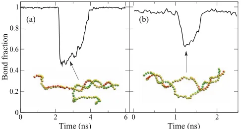
FIG. 13. A 50-bp poly-AT DNA in partially molten states: (a) unzipping from one end, and (b) formation of a bubble. Insets show snapshots of the molecule; the color schemes are the same as in Fig.10.

sudden extension is less. The superstretching transition is a very stringent test for our computational model, as it involves strong departures from the equilibrium structure. Notwith-standing the neglect of solvent interactions and the athermal character, our coarse-grained potential still provides reason-able results under such critical conditions. Simulations also reveal that the superstretching is accompanied by unwinding of the double helix, as shown in Fig.12. Above the critical force, our model shows that the DNA is twisted slightly in the left-handed direction.

D. Bubble formation

Although our potentials are formulated for ds-DNA, in some applications it is desirable to have a model that can ac-count for broken hydrogen bonds. Here, we test the validity of our model when the double strand in a 50-bp poly-AT DNA is partially broken. The onset of melting can be observed in our model, but the melting temperature is overestimated. At temperature 550 K, the double-strand shows occasional un-zipping; one instance is shown in Fig.13(a). At 800 K, for-mation of bubbles can be observed; one instance is shown in Fig. 13(b). The overestimation of melting temperature may arise from several reasons. First, our stacking potential is not formulated for single strands or strands with broken hydrogen bonds. Second, the presence of water molecules may lower the energy of the broken-bond states, but this effect is not taken into account. Third, the coarse-grained potentials here are derived at zero temperature, which is stiffer than at finite temperature. However, the appearance of these intermediate molten states is still an indication that our model is stable be-yond strictly ds-DNA structures.

VI. CONCLUSION

configurations of random DNA sequences and can be used to model related biophysical processes. Unavoidably, some sim-plifying assumptions were used in the model formulation and construction. In order to use a minimal number of empirical terms, only the effect of ionic screening was added to the mi-croscopically derived potential. At a later stage, such empiri-cal term can be replaced by a more microscopic approach.63

A series of tests were performed, and they verified that the coarse-grained potential can reproduce the stable B-DNA structure, and that the predicted structure matches the known crystallographic structure of DNA to a few % in key structural parameters. The model produces persistence lengths in close agreement with experimental data, and the response of the persistence length to varying salt concentrations also agrees with the prediction for a linked-cylinder model. These tests suggest that the mechanical properties of the coarse-grained model will show realistic trends when subject to the complex electrokinetic environment in the cell or in artificial systems such as the interior of an nanochannel during translocation experiments.

The tests on overstretching and on bubble formation show that the model may capture the qualitative features in such states, but also reveal some limitations of the model. To describe such states accurately, we may need a more realis-tic account of the solvent molecules and of the temperature dependence of the coarse-grained potentials. This will be the subject of future work. Other possible and more straightfor-ward extensions of the current model will be to formulate the stacking interaction to work with ss-DNA, and to parametrize interactions for mismatched base-pairs and for uracil (to ex-tend the model to RNA). Also, the current model does not ac-count for inter-strand interactions except for the electrostatic repulsion, and so situations like long DNA strands under con-finement may not be appropriate for this model.

The approach described in this work is attractive for de-scribing ds-DNA using a minimal of empirically derived pa-rameters and with a good compromise between accuracy and computational efficiency. We suggest that this model could be a useful tool for simulating the behavior of ds-DNA in a va-riety of biologically relevant or device-related scenarios with modest computational resources.

ACKNOWLEDGMENTS

The authors thank Sheng Meng and Wei Li Wang for a critical reading of the manuscript, and acknowledge G.N. Patey for helpful comments and discussions. C.W.H. thanks Wei Li Wang for his kind helps and fruitful discussions. M.F. acknowledges support by Harvard’s Nanoscale Science and Engineering Center, funded by the National Science Founda-tion, Award Number PHY-0117795. G.L. acknowledges sup-port from the post-doctoral fellowship program of the Natural Science and Engineering Research Council of Canada.

1_{H. Lodish, A. Berk, C. A. Kaiser, M. Krieger, M. P. Scott, A. Brestscher, H.} Ploegh, and P. Matsudaira,Molecular Cell Biology, 6th ed. (W. H. Freeman and Company, New York, 2007).

2_{A. D. MacKerell, J. Wiorkiewicz-Kuczera, and M. Karplus,J. Am. Chem.} Soc.117, 11946 (1995).

3_{R. Laveryet al.,Nucleic Acids Res.38, 299 (2010).}

4_{D. Brantonet al.,Nat. Biotech.26, 1146 (2008).}

5_{M. Fyta, S. Melchionna, and S. Succi,J. Polym. Sci., Part B: Polym. Phys.}

49, 985 (2011).

6_{H. L. Dormann, B. S. Tseng, C. D. Allis, H. Funabiki, and W. Fischle,Cell} Cycle5, 2842 (2006).

7_{H. Y. Liu, M. Elstner, E. Kaxiras, T. Frauenheim, J. Hermans, and W. Yang,} Proteins: Struct. Funct. Genet.44, 484 (2001).

8_{R. L. Barnett, P. Maragakis, A. Turner, M. Fyta, and E. Kaxiras,J. Mater.} Sci.42, 8894 (2007).

9_{K. Drukker and G. C. Schatz,J. Phys. Chem. B 104, 6108 (2000); K.} Drukker, G. Wu, and G. C. Schatz,J. Chem. Phys.114, 579 (2001). 10_{R. M. Jendrejack, J. J. de Pablo, and M. D. Graham,J. Chem. Phys.116,}

7752 (2002).

11_{B. D. Coleman, W. K. Olson, and D. Swigon,J. Chem. Phys.118, 7127} (2003).

12_{H. L. Tepper and G. A. Voth,J. Chem. Phys.122, 124906 (2005).} 13_{F. W. Starr and F. Sciortino,J. Phys.: Condens. Matter18, L347 (2006).} 14_{T. A. Knotts IV, N. Rathore, D. C. Schwartz, and J. J. de Pablo,J. Chem.}

Phys.126, 084901 (2007).

15_{P. D. Dans, A. Zeida, M. R. Machado, and S. Pantano,J. Chem. Theory} Comput.6, 1711 (2010).

16_{T. E. Ouldridge, A. A. Louis, and J. P. K. Doye,Phys. Rev. Lett.104,} 178101 (2010).

17_{M. C. Linak, R. Tourdot, and K. D. Dorfman,J. Chem. Phys.135, 205102} (2011).

18_{A. Savelyev and G. A. Papoian,Biophys. J.96, 4044 (2009).}

19_{M. Maciejczyk, A. Spasic, A. Liwo, and H. A. Scheraga,J. Comput. Chem.}

31, 1644 (2010).

20_{S. M. Gopal, S. Mukherjee, Y. M. Cheng, and M. Feig,Proteins78, 1266} (2010).

21_{A. Morriss-Andrews, J. Rottler, and S. S. Plotkin, J. Chem. Phys.132,} 035105 (2010).

22_{N. B. Becker and R. Everaers,Phys. Rev. E76, 021923 (2007).} 23_{N. B. Becker and R. Everaers,J. Chem. Phys.130, 135102 (2009).} 24_{E. J. Sambriski, D. C. Schwartz, and J. J. de Pablo,Biophys. J.96, 1675}

(2009).

25_{E. J. Sambriski, V. Ortiz, and J. J. de Pablo,J. Phys.: Condens. Matter21,} 034105 (2009).

26_{E. J. Sambriski, D. C. Schwartz, and J. J. de Pablo,Proc. Natl. Acad. Sci.} U.S.A.106, 18125 (2009).

27_{M. J. Hoefert, E. J. Sambriski, and J. J. de Pablo,Soft Matter7, 560 (2010).} 28_{V. Ortiz and J. de Pablo,Phys. Rev. Lett.106, 238107 (2011).}

29_{A.-M. Florescu and M. Joyeux,J. Chem. Phys.135, 085105 (2011).} 30_{R. C. DeMille, T. E. Cheatham III, and V. Molinero,J. Phys. Chem. B115,}

132 (2011).

31_{T. E. Ouldridge, I. G. Johnston, A. A. Louis, and J. P. K. Doye,J. Chem.} Phys.130, 065101 (2009).

32_{C. W. Hsu, J. Largo, F. Sciortino, and F. W. Starr,Proc. Natl. Acad. Sci.} U.S.A.105, 13711 (2008); W. Dai, C. W. Hsu, F. Sciortino, and F. W. Starr, Langmuir26, 3601 (2010); C. W. Hsu, F. Sciortino, and F. W. Starr,Phys. Rev. Lett.105, 055502 (2010).

33_{T. E. Ouldridge, A. A. Louis, and J. P. K. Doye,J. Chem. Phys.134, 085101} (2011).

34_{A. Savelyev and G. A. Papoian,Proc. Natl. Acad. Sci. U.S.A.107, 20340} (2010).

35_{P. Hohenberg and W. Kohn,Phys. Rev.136, B864 (1964); W. Kohn and L.} J. Sham,ibid.140, A1133 (1965).

36_{J. M. Soler, E. Artacho, J. D. Gale, A. García, J. Junguera, P. Ordejón, and} D. Sánchez-Portal,J. Phys.: Condens. Matter14, 2745 (2002).

37_{A. Hübsch, R. G. Endres, D. L. Cox, and R. R. P. Singh,Phys. Rev. Lett.94,} 178102 (2005); H. Wang, J. P. Lewis, and O. F. Sankey,ibid.93, 016401 (2004);85,4992(2000); R. E. A. Kelly and L. N. Kantorovich,J. Phys. Chem. C111, 3883 (2007); S. Meng, W. L. Wang, P. Maragakis, and E. Kaxiras,Nano Lett.7, 2312 (2007).

38_{A. Tsolakidis and E. Kaxiras,J. Phys. Chem. A 109, 2373 (2005); D.} Varsano, R. Di Felice, M. A. L. Marques, and A. Rubio,J. Phys. Chem. B110, 7129 (2006).

39_{N. Trouiller and J. L. Martins,Phys. Rev. B43, 8861 (1991).}

40_{J. P. Perdew, K. Burke, and M. Ernzerhof,Phys. Rev. Lett.77, 3865 (1996).} 41_{J. Ireta, J. Neugebauer, and M. Scheffler,J. Phys, Chem. A 108, 5692}

(2004).

42_{T. van der Wijst, C. F. Guerra, M. Swart, and F. M. Bickelhaupt,Chem.} Phys. Lett.426, 415 (2006).

44_{J.Šponer, J. Leszczy´nski, and P. Hobza,J. Phys. Chem.100, 5590 (1996).} 45_{P. Hobza, J.Šponer, and M. Polasek,J. Am. Chem. Soc.117, 792 (1995).} 46_{E. R. Johnson, I. D. Mackie, and G. A. DiLabio,J. Phys. Org. Chem.22,}

1127 (2009).

47_{Q. Wu and W. Yang,J. Chem. Phys.116, 515 (2002).}

48_{M. Dion, H. Rydberg, E. Schröder, D. C. Langreth, and B. I. Lundqvist,} Phys. Rev. Lett.92, 246401 (2004).

49_{S. F. Boys and F. Bernandi,Mol. Phys.19, 553 (1970).}

50_{W. T. M. Mooij, F. B. van Duijneveldt, J. G. C. M. van Duijneveldt-van de} Rijdt, and B. P. van Eijck,J. Phys., Chem. A103, 9872 (1999).

51_{A. Banerjea and J. R. Smith,Phys. Rev. B37, 6632 (1988).} 52_{J. Mazur and R. L. Jernigan,Biopolymers31, 1615 (1991).} 53_{S. H. Lee and J. C. Rasaiah,J. Phys. Chem.100, 1420 (1996).}

54_{G. L. Randall, L. Zechiedrich, and B. Montgomery Pettitt,Nucl. Acids Res.}

37(16), 5568 (2009).

55_{M. E. Tuckerman, B. J. Berne, and G. J. Martyna,J. Chem. Phys.97, 1990} (1992).

56_{S. Melchionna,J. Chem. Phys.127, 044108 (2007).}

57_{S. Arnott, P. J. C. Smith, and R. Chandrasekaran, inCRC Handbook of} Bio-chemistry and Molecular Biology, 3rd ed., edited by G. D. Fasman (CRC, Cleveland, 1976), Vol. 2, pp. 411–422.

58_{N. Narayana and M. A. Weiss,J. Mol. Biol.385, 469 (2009).}

59_{C. G. Baumann, S. B. Smith, V. A. Boomfield, and C. Bustamante,Proc.} Natl. Acad. Sci. U.S.A.94, 6185 (1997).

60_{J. Skolnick and M. Fixman,Macromolecules10, 944 (1977).}

61_{P. Cluzel, A. Lebrun, C. Heller, R. Lavery, J.-L. Viovy, D. Chatenay, and} F. Caron,Science271, 792 (1996).

62_{S. B. Smith, Y. Cui, and C. Bustamante,Science271, 795 (1996).} 63_{S. Melchionna and U. Marini Bettolo Marconi,Europhys. Lett.95, 44002}