Estimation of effective connectivity via data-driven neural modeling

Estimation of effective connectivity via data-driven neural

modeling

Dean R. Freestone1,2_*†_{, Philippa J. Karoly}1,2†_{, Dragan Neši ´c}2_{, Parham Aram}3_{, Mark J. Cook}1_and

David B. Grayden2,4

1

Department of Medicine, St. Vincent’s Hospital Melbourne, The University of Melbourne, Fitzroy, VIC, Australia

2

NeuroEngineering Laboratory, Department of Electrical and Electronic Engineering, The University of Melbourne, Parkville, VIC, Australia

3

Department of Automatic Control and Systems Engineering, University of Sheffield, Sheffield, UK

4

Centre for Neural Engineering, The University of Melbourne, Parkville, VIC, Australia

Edited by:

Patrick William Carney, The Florey Institute of Neuroscience and Mental Health, Australia

Reviewed by:

Klaus Lehnertz, University of Bonn, Germany

Bruce Gluckman, Penn State University, USA

*Correspondence:

Dean R. Freestone, Department of Medicine, St. Vincent’s Hospital Melbourne, The University of Melbourne, 19 Regent St., Fitzroy, VIC 3065, Australia

e-mail: [email protected]

†These authors have contributed equally to this work and share first authorship.

This research introduces a new method for functional brain imaging via a process of model inversion. By estimating parameters of a computational model, we are able to track effective connectivity and mean membrane potential dynamics that cannot be directly measured using electrophysiological measurements alone. The ability to track the hidden aspects of neurophysiology will have a profound impact on the way we understand and treat epilepsy. For example, under the assumption the model captures the key features of the cortical circuits of interest, the framework will provide insights into seizure initiation and termination on a patient-specific basis. It will enable investigation into the effect a particular drug has on specific neural populations and connectivity structures using minimally invasive measurements. The method is based on approximating brain networks using an interconnected neural population model. The neural population model is based on a neural mass model that describes the functional activity of the brain, capturing the mesoscopic biophysics and anatomical structure. The model is made subject-specific by estimating the strength of intra-cortical connections within a region and inter-cortical connections between regions using a novel Kalman filtering method. We demonstrate through simulation how the framework can be used to track the mechanisms involved in seizure initiation and termination.

Keywords: functional connectivity, neural mass model, model inversion, Kalman filter, epilepsy, seizures, parameter estimation, effective connectivity

1. INTRODUCTION

This paper presents a model-based framework for imaging neu-ral dynamics from electrophysiological data. This paper builds on a rich history of research in computational neuroscience that has been increasingly focused on the development of generative models to understand the link between neural activity and neu-roimaging data (David et al., 2004; Coombes and Terry, 2012; Moran et al., 2013), with emphasis on two main areas. The first area of focus is forward modeling, or the mapping of relevant neuronal variables to recorded data that facilitates the devel-opment of theoretical predictions. The second area of focus is inverse modeling, which is the prediction of states, parameters and neuronal outputs given measured data (David, 2007). The new research presented in this manuscript provides a framework that contributes to solving the inversion problem. A key contri-bution of this paper is the development of an estimation scheme that is applicable to many alternate neural architectures that can be described by a core set of equations, which encapsulates our knowledge of the biophysics of large-scale neural systems.

Large-scale neural models can combine information from multiple neuroimaging modalities (fMRI, EEG, MEG, etc.), allowing a systems approach for data analysis. The behavior of such models is described by system states, whose dynamics are set

by parameters, which are static variables. The systems approach of conducting analyses allows one to study all interactions as a whole. This has advantages over correlation-based science, where correlations do not necessarily reveal causation in large-scale sys-tems. A systems approach provides a unified picture of both local properties and remote interactions, and is considered crit-ical to form an understanding of many of the brain’s activities (Freeman, 1975; Deco et al., 2008) including seizure generation (Wendling et al., 2000; Breakspear et al., 2006), which is the focus of this study. In the context of this study, the local properties are described by the connectivity strengths between neural subtypes within the circuitry of a functional processing unit (cortical area or cortical column) and the remote interactions are the functional changes that occur between cortical areas.

to the specific functional requirements of the brain through tem-poral and spatial fluctuations in their interrelationships (da Costa and Martin, 2010). The neural mass model (Jansen and Rit, 1995) that is used for inferring connectivity in this current study can be considered a simplified form of a canonical cortical circuit.

For biological systems, structure is usually a good starting point to study functional interactions (Crick and Koch, 2005). For the brain, this process usually starts with building a map of the anatomic pathways (Sporns, 2013; Van Essen et al., 2013). Often quite separately from the anatomical data, functional rela-tionships are also analyzed through temporal correlations in neu-roimaging data, which is recorded from spatially distinct regions of the brain. For example, PET, fMRI, and EEG data have all been used to infer connectivity within and between regions of cor-tex using a variety of quantitative measures (Biswal et al., 1995; Horwitz et al., 1995; Bokde et al., 2001; Horwitz, 2003). A major challenge lies in consolidating the anatomical data and the func-tional data to form a unified causative model. This challenge is addressed by the framework presented in this paper.

This paper is concerned with the investigation of effective con-nectivity through causal modeling. In the context of this paper, effective connectivity is defined as the influence one neural area has on another (Friston, 1994). It is anticipated that the use of causal models, which encapsulate our knowledge of the anatom-ical connectivity and biophysics of neural populations in con-junction with experimental measurements, will provide a more complete picture of how neural connectivity mediates function. The generation of patient-specific models will also be benefi-cial in a clinical context, providing greater insight into the cause and progression of neurological disorders, such as epilepsy, and enabling treatment regimes to be investigated through computer simulations.

Analysis of mesoscopic neural dynamics through the use of mean-field models has been validated through several alter-native approaches. For example, the so-called neural mass model (Wilson and Cowan, 1972; Da Silva et al., 1974; Freeman, 1987) has been able to describe a large range of neural dynam-ics such as alpha rhythms (Jansen and Rit, 1995), MEG/EEG oscillations (David and Friston, 2003) and epileptic activ-ity (Wendling et al., 2002). Neural mass models can also be easily extended to define additional population types and larger cortical regions (Babajani-Feremi and Soltanian-Zadeh, 2010; Cui et al., 2011; Goodfellow et al., 2011). The aforementioned results motivate the use of the neural mass model as the basis of a canonical cortical circuit. Furthermore, neural mass mod-els offer a reasonable trade-off between biological realism and parsimony, allowing for practical implementation and subse-quent inversion. Inversion is the key to using recorded data to estimate the neural states (membrane dynamics of various neu-ral population subtypes) and parameters (defining connectivity strengths). Estimation of system variables provides new infor-mation about underlying population dynamics and physiological properties that cannot be directly measured using other neu-roimaging methods (without destroying the tissue). For instance, the connectivity strength between neural population subtypes (i.e., pyramidal, spiny stellate and inhibitory interneurons) have been implicated in seizure generation and have also been found to

be patient-specific (Wendling et al., 2000; Breakspear et al., 2006; Blenkinsop et al., 2012).

It has previously been demonstrated that a model-based neu-rophysiological framework can be used to image parameters associated with seizure onset, evolution and termination in an individual epilepsy patient using ECoG data (Freestone et al., 2013). The framework presented in this manuscript builds on this with improvements to the estimation algorithm and an expansion to include multiple brain regions. Numerous other formulations exist for fitting spatially extended mesoscopic neural models to data. For instance, dynamic causal modeling (DCM) is a tech-nique that is often applied to investigate connectivity of neural areas using generative models (Friston et al., 2003; Kiebel et al., 2006). DCM applies Bayesian inference to determine the most probable configuration of model parameters (i.e., neural cou-pling coefficients) given a window of recorded data. Therefore, the resulting model is contextualized by the experimentally applied stimuli or conditions under which data was generated (Daunizeau et al., 2011). Another approach has been to apply genetic algo-rithms to search the parameter space of the model for a structure that is optimal for generating the observed data (Wendling et al., 2005; Nevado-Holgado et al., 2012). In relation to the current work, the aforementioned methods of model optimization can be used to initialize the inversion technique outlined in this paper.

The inversion method outlined in this paper is based on the Kalman filter (Kalman, 1960). The model dynamics are assumed to adhere to a Markov process and estimation quantities (states and parameters) are approximated as random variables with Gaussian distributions. For every electrocorticography (ECoG) measurement, the multivariate state and parameter distribution is propagated through the neural population model; then Bayes rule is used to determine the posterior probability distribution of parameters given measured data. In the case of a linear model, this method is known as the augmented Kalman filter, which provides the optimal (minimizing the variance of the estimation errors) unbiased estimate for states and parameters. Various ver-sions of the Kalman filter equations for nonlinear models have been previously applied for model inversion (Voss et al., 2004; Schiff and Sauer, 2008; Deng et al., 2009; Freestone et al., 2011; Aram et al., 2013; Liu and Gao, 2013). However, these stud-ies were based on either simplified field equations or a single region population model. A key advantage of the Kalman filter-based estimation algorithm outlined in this paper over other expectation maximization or genetic algorithm type schemes is the ability to track states and parameters in real time. Tracking in real time provides a greater level of temporal accuracy in the detection of transitions that underly specific neural activity (such as seizure generation). Furthermore, this paper demon-strates a flexible predictive framework that can be readily adapted to alternative forms of the neural population model (that are based on the same fundamental building blocks) in order to reflect our most current understanding of the architecture of the brain.

subject-specific data. Next, example simulations and results are provided that validate the framework for both single and multiple cortical areas. We then provide an example specific to study-ing epilepsy, where we show how the framework can be used to identify a seizure onset site and the mechanism for seizure ini-tiation and termination. The final section discusses the benefits of this approach in a wider context of understanding seizures and developing much needed new therapies as well as the current limitations of the proposed framework and directions for further work.

2. MATERIALS AND METHODS

This section discusses the core biophysics of the mass action of the cortical regions that are incorporated into our mathemati-cal model along with the algorithm for tailoring the model to subject-specific data. Together, the mathematical model and the estimation algorithm form a lens that focuses on the parameters that govern connectivity and function of neural networks.

2.1. NEURAL POPULATION MODEL

The neural population model that is used for the framework is based on the neural mass model. This type of neural model describes the dynamics of the mean membrane potential of a population of a specific neuron subtype given firing rate inputs. Populations of this type with varied parameters can be connected together to form local networks to describe the dynamics of spe-cific cortical regions, such as a cortical column. Multiple cortical regions can then be interconnected to form a large-scale net-work model. Within this section, the building blocks of all neural populations of our large-scale network model are presented that describe the action of the synaptic connections (mean firing rate to mean membrane potential) and the action of the somas (mean membrane to firing rate). The notation used to derive the neu-ral population model in the following section is summarized in Table 1.

Table 1 | Notation for the neural population model.

Notation Interpretation

αmn Connectivity parameter, populationmton

vmn Post-synaptic potential

zmn Derivative of post-synaptic potential

vn Net mean membrane potential for populationn

hmn(t) Post-synaptic response kernel

φm Mean firing rate

g(_·) Sigmoidal activation function

u Input from external unmodeled population

τmn Synaptic time constant

ς Standard deviation of firing thresholds

v0 Mean firing threshold

M Total number of populations in the model

N Total number of intra-region connections

J Total number of regions in the model

K Total number of inter-region connection

δ Time step

2.1.1. Single population model

To derive a population model, we begin by defining the mean membrane potential of a neural population, vn, as the sum of contributing mean post-synaptic potentials,vmn, where the post-synaptic and pre-post-synaptic neural populations are indexed by n andm, respectively,

vn= M

m=1

vmn. (1)

Each post-synaptic potential arises from the convolution of the input firing rate,φm(t), with the post-synaptic response kernel

vmn(t)= αmn_−∞t hmn(t−t)φm(t) dt, (2)

whereαmnis a lumped connectivity parameter that incorporates the average synaptic gain, the number of connections and the average maximum firing rate of the presynaptic populations. All lumped connectivity parameters are assumed to be unknown, so must be inferred from data. The post-synaptic response kernels denoted byhmn(t) describe the profile of the post-synaptic mem-brane potential of populationnthat is induced by an infinites-imally short pulse from the inputs (like an action potential). The post-synaptic response kernels are parameterized by the time constantτmnand are given by

hmn(t)=η(t) t τmn

exp

−_τt mn

, (3)

where η(t) is the Heaviside step function. Typically, αmn and

τmnare assumed to be constants (particularly for current-based synapses) that define the presynaptic population type. For exam-ple, GABAergic inhibitory interneurons typically induce a higher amplitude post-synaptic potential with a longer time constant than glutamatergic excitatory cells. For the model that we are con-sidering, the indexn(post-synaptic) may represent either pyra-midal (p), excitatory interneuron (spiny stellate) (e) or inhibitory interneuron (i) populations.

The inputs to the population,φmn, may come from external regions,u, or from other populations within the model,gmn(vm), where

φm=

um ifmindexes external inputs

g(vm)ifmindexes internal inputs . (4)

g(vm)= √1 2πς

vm

−∞exp

−(z−v0)2

2ς2 dz (5)

= 1 2

erf

vm−v0

√ 2ς

+1

. (6)

The quantity ς describes the slope of the sigmoid or, equiva-lently, the variance of firing thresholds of the presynaptic pop-ulation (assuming a Gaussian distribution of firing thresholds). The mean firing threshold relative to the mean resting mem-brane potential is denoted byv0(v0=vthresh+vrest). The resting

membrane potential is not usually explicitly defined for forward models of this type. However, for inverse models, it is important to understand how the resting membrane potential is included in the equations. The parameters of the sigmoidal activation functions,ςandv0, are usually assumed to be constants.

The convolution in Equation 2 can conveniently be written as two coupled, first-order ordinary differential equations, which is a second-order state-space model. This gives the system

dvmn dt =zmn dzmn

dt =

αmn

τmnφmn− 2 τmnzmn−

1 τ2

mn

vmn. (7)

In summary, this single neural population model maps from a mean pre-synaptic firing rate to a post-synaptic potential. The terms that are usually considered parameters of the model are the synaptic time constants, τ, the connectivity constants, α,

the mean firing thresholds,v0, and firing threshold variances,ς.

These parameters can be set to describe connections between spe-cific neural populations, such as pyramidal neurons, spiny stellate cells and fast and slow inhibitory interneurons.

2.1.2. Multiple populations for a cortical region

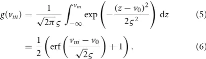
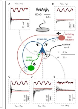
Multiple populations in the form of Equation 7 can be config-ured and interconnected to represent the circuitry of a cortical region, such as a cortical column. Each synaptic connection in the model is described by the set of coupled first-order ODEs of Equation 7; however, the parameters are connection-specific. Models exist in the literature describing from two to five different neural types with two to thirteen synaptic con-nections (4th to 26th order) (Da Silva et al., 1974; Wang and Knösche, 2013). Contributions in this regard have been made by David and Friston (2003); Wendling et al. (2002); Jansen and Rit (1995) and others. An illustration of the model of a cortical region used in this study is shown in Figure 1.

The parameters of the neural populations not only define the population type, but also the behavior the model of the cortical region exhibits. For example, for a certain parameter combination, we obtain a model of a cortical region that will generate alpha-wave type activity; for another set of parameters, we obtain a different model that will exhibit epileptic behavior. The parameters used in this study have been determined previ-ously for similar models (Jansen and Rit, 1995) and are shown inTable 2. The parameters to be estimated are the synaptic gain terms,αmn.

FIGURE 1 | Population model of a cortical region.The left hand side shows a cross section of the cortical laminar, highlighting the stratification and different population the various layers. A graphical representation of the population model is presented on the right hand side, showing three interconnected neural populations, which are inhibitory interneurons (supragranular layers), excitatory spiny stellate cells (granular layer), and

pyramidal neurons (infraganualar layers). The specific subtype of neural population is defined by the parameters that describe the post-synaptic response kernels. The intra-region connectivity are denoted byαmn, where

Table 2 | Fixed parameter values for the neural population model that are not estimated.

Parameter Value

ς 3 mV

v0 6 mV

τup,τpe,τpi,τep 10 ms

τip 20 ms

τd 30.3 ms

um 220

σ2

u 5.74

δ 1 ms

2.1.3. Multiple region model

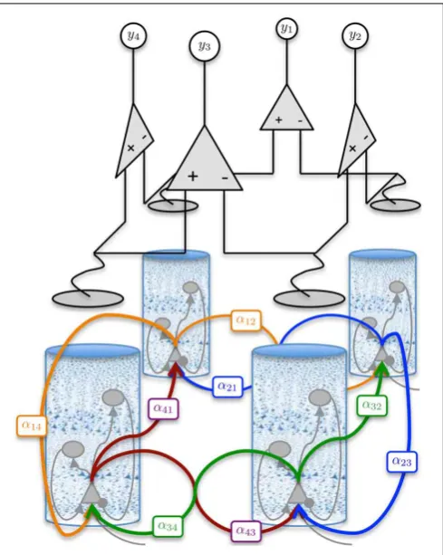
Coupling of cortical regionjto regionkis achieved by connect-ing the output firconnect-ing rate of the pyramidal population in region jto the input of the pyramidal population in regionkvia a delay kernel. The delay kernel is of the same form as the post-synaptic response kernel of Equation 3, but maps a firing rate to a delayed firing rate. The inputs from the delayed firing rates are modeled for every pyramidal population using the same form of second-order model defined in Equation 7. All interconnections between regions were assumed to have the same delay kernel, which was parameterized by a time constant, τd (Wendling et al., 2000) (see Table 2). The delayed firing rates form standard inputs to the pyramidal cells in the adjoining cortical region and induce post-synaptic potentials via a convolution kernel as described by Equation 2. However, the connectivity parameterαjkdescribes the interconnection gain between regions rather than between pop-ulations. In this study, we consider four interconnected cortical regions as shown inFigure 2. The values of the interconnection gains for forward simulations were tuned to achieve the desired behavior in the ECoG outputs, while avoiding saturation of neu-ral populations. Different interconnection gains were used to either simulate data consistent with alpha rhythms or to achieve transition to seizure. Further details about the simulations and parameters used are given in Section 2.3.

2.1.4. Augmented discrete time state-space model

For notational convenience, the subscripts for the synaptic gains, denoted αmnandαjk, and the post-synaptic potentials, denoted byvmnin the previous section, will now be numbered sequentially from 1 toN+K.Nis the number of intra-regional connections andKis the number of inter-regional connections in the multi-area model.

The state vector is a concatenation of discrete time values of the post-synaptic membrane potentials, the derivatives of the poten-tials, the delayed firing rates (inter-region) and their derivatives by

xv1z1. . .vN zN vφ,1 zφ,1 . . .vφ,K zφ,K

_,

where the large-scale model hasN intra-region connections and K inter-region connections. The subscript φ indicates that the post-synaptic potential/derivative is associated with the delayed firing rate from a pyramidal population of a neighboring region.

FIGURE 2 | Graphical representation of the four region population model with differential ECoG measurements.Each region is interconnected to its immediate neighbor. The inter-region connectivity strength is governed by the parameterαjk, wherejandk∈ {1,2,3,4}and

j=k. The differential montage provides a more realistic measurement model then what is typically used for model inversion.

The parameters to be estimated can also be concatenated into a vector by

θ αl,1 . . . αl,N αd,1 . . . αd,K

,

whereldenotes local connections within regions (including from inputs,u),ddenotes distant connections between regions. For a four-region model, assuming the number of connections within each region is equal, then the number of connections within each region is equal toN÷4. In this formulation of the model the parameter vector is written in differential form, with trivial dynamics as

˙

θ =0. (8)

The differential form of the parameter vector facilitates augment-ing the parameters to the state vector for estimation purposes.

The augmented state space vector is created by

which has dimensionality ξ∈Rnξ _{where nξ=3(N+K). The} augmented large-scale state space model is given by

˙

ξ =Aξ+Bξ◦g(Cξ)+D(u)ξ, (10)

where◦denotes element-wise multiplication. The matricesA,B, C, andD(u) are defined in Appendix 5.2. The large-scale model can be written in a compact form that is useful for deriving the estimation algorithm by

˙

ξ=F(ξ,u) . (11)

It is necessary to discretize the model for estimation purposes. The Euler method was used for discretizing the model and is pre-sented in Appendix 5.1. For the Bayesian inference scheme, it is also necessary to model uncertainty in our model by an additive noise term. With the inclusion of the additive noise term,wt, the discrete time augmented state space model is denoted by

ξt+1=Aδξt+Bδξt◦g

Cξt

+Dδ(ut)ξt+wt (12)

and can be written in compact form by

ξt+1=Fδ

ξt,ut+wt. (13)

The model uncertainty is defined by a zero mean, temporally white Gaussian with known covariance matrix Q. In forward models,wtis used as a driving term to simulate unknown input to the system from afferent connections or from other cortical regions. However, for model inversion purposes, this additional term also facilitates estimation and tracking of parameters via Kalman filtering or other Bayesian inference schemes. For the Kalman filter, the covariance ofwtquantifies the error in the pre-dictions through the model. If we believed our model is accurate, then we would set all of the elements ofQto a small value. On the other hand, a high degree of model-to-brain mismatch can be quantified by setting the elements ofQto larger values.

2.1.5. Model of ECoG measurements

It is well accepted that the field potentials that are measured with ECoG are predominately generated by synaptic currents arising from inputs to the pyramidal neurons (Nunez and Srinivasan, 2006). In our model, these currents are linearly proportional to the mean membrane potential of the pyramidal population. Therefore, the ECoG signal is modeled as the mean membrane potential of the pyramidal population, which is the sum of the incoming post-synaptic membrane potentials.

For the multi-region neural population the ECoG measure-ment is taken to be the difference between neighboring regions. This provides a differential montage that is compatible with experimental data. Typically, the generators of ECoG signals are modeled by the individual mean membrane potentials of the pyramidal populations, effectively ignoring the differential nature of actual ECoG recordings. In this paper, we demonstrate that parameters can be accurately estimating when using the more realistic measurement model.

The measurement model that relates the ECoG measurements to the augmented state vector,ξt, is given by

yt =Hξt+vt, (14)

where vt∼N(0,R) is a zero mean, spatially and temporally white Gaussian noise process with a standard deviation of 1 mV, that simulates measurement errors. For model inversion pur-poses, the variance ofvt quantifies the confidence we have in the measurements. The matrixHdefines a summation of the mem-brane potentials (corresponding to pyramidal populations) that contribute to each ECoG channel along with the differential mon-taging scheme. The number of channels used in this case was equal to the number of regions (four), as seen inFigure 2.

2.2. A KALMAN FILTER FOR THE POPULATION MODEL

The aim of the Kalman filter is to estimate the most likely sequences of states,ξˆ+t , and the associated error covariances,Pˆ+t , given (uncertain) knowledge of the biophysics and anatomy of the brain regions of interest combined with the noisy ECoG mea-surements,yt. The optimal state estimates can be formally stated using the expectations

ˆ ξ+t =E

ξt|y1,y2, . . . ,yt

(15)

ˆ

P+t =E

(ξt− ˆξ

+

t )(ξt− ˆξ

+

t )

, (16)

which are known as the a posteriori state estimate and state esti-mate covariance, respectively. The a posteriori state estiesti-mate is computed by correcting the a priori state estimate, which is a prediction though our model and defined as

ˆ ξ−t =E

ξt|y1,y2, . . . ,yt−1, (17)

using a weighted difference between a prediction of the observa-tions and the actual noisy measurements. The a posteriori state estimate is calculated by updating the prediction using measured data by

ˆ ξ+t = ˆξ

−

t +Kt

yt−Hξˆ

−

t

ECoG prediction error

. (18)

The weighting to correct the a priori augmented state estimate,

Kt, is known as the Kalman gain (Kalman, 1960). The Kalman gain is calculated using the available information regarding the confidence in a prediction of the augmented states through the model and the observation model that includes noise by

Kt= ˆP−t H

HPˆ−_t H+R−1, (19)

where

ˆ

P−t =E

ξt− ˆξ

−

t ξt− ˆξ

−

t

is the a priori state estimate error covariance,Ris the observation noise covariance, and His the observation matrix. For a linear observation function, the a posteriori covariance is then updated by using the Kalman gain to provide the correction

ˆ

P+t =(I−KtH)Pˆ−t . (21)

Practically, the actual state is not known so the Kalman filter must be initialized with the best guess forξˆ+0 andPˆ+0, which provides

the a posteriori state estimate and state estimate covariance for timet=0. The a priori state estimate for timet=1 can then be computed by propagating the initial guess through the model and taking the expectation,

ˆ ξ−t =E

Fδ

ˆ

ξ+t−1,ut−1

(22)

=EAδξˆ+t−1+Bδξˆ +

t−1◦g

Cξˆ+_t−1+Dδ(ut−1)ξˆ +

t−1

(23)

=Aδξˆ+t−1+E

Bδξˆ+t−1◦g

Cξˆ+t−1

+Dδ(ut−1)ξˆ +

t−1(24)

Generally, for nonlinear systems, the solution to this expectation is not known. Therefore, approximations are often used, such as the extended and unscented Kalman filters, respectively.

We approximate the expectation by

EBδξˆ+t−1◦g

Cξˆ+t−1

≈Bδξˆ+t−1◦E

gCξˆ+t−1

, (25)

where the accuracy of the approximation depends on the width of the distributions for the parameters,Bξ+_t−1. Since we are assum-ing the parameters are unknown with the possibility of slow changes, a small amount of uncertainty is added. For known parameters, Equation 25 would be exact. Therefore, the accuracy of the approximation improves as parameter estimates converge toward their actual values.

In an effort to improve state and parameter estimation accu-racy, a new innovation in this study is an analytic solution to the expectation of the mean membrane potential, which is modeled as a Gaussian, transformed by the sigmoid. To show the solution, we first point out that

γjξˆ

+

t−1= ˆvt,j (26)

corresponds to the total pre-synaptic mean membrane poten-tial of the jth neural population, where γj is a row vector from the adjacency matrix, C, which is described in detail in Appendix 5.2. Also, the variance of the pre-synaptic mean mem-brane potential is

γjPˆ+t−1γj = ˆσt2,j. (27)

The analytic solution for the expectation of a Gaussian distributed random variable (total membrane potential of the respective pop-ulation) transformed by the sigmoid error function, g(·), is given by

Egγjξˆ

+

t−1

=1 2 ⎛ ⎜ ⎜ ⎝erf ⎛ ⎜ ⎜ ⎝ γj

ˆ

ξ+t−1−v0

2ς2_+γ

jPˆ+t−1γj

⎞ ⎟ ⎟ ⎠+1

⎞ ⎟ ⎟ ⎠.(28)

The derivation of this new result is shown in Appendix 5.3. The a-priori covariance is approximated using the unscented transform, which approximates the statistics of a multivariate Gaussian that undergoes a nonlinear transformation (Julier and Uhlmann, 1997). The approximation is given by

ˆ

P−t ≈

2nx

i=0

WifXit−1,u

− ˆξ−t f

Xi t−1,u

− ˆξ−t

,

(29)

where Xit−1 is a matrix of sigma vectors, which are carefully

chosen samples from the distribution ofxˆ+_t−1, andWi are vec-tors of weights associated with the transform. For completeness, the method of computing the sigma vectors and the weights is provided in Appendix 5.4.

It is likely that the parameters and states described by a cortical circuit will be subject to identifiable physiological constraints that should be included in an inversion problem in order to exploit all available information. There are various ways to constrain the parameter space by truncating the distribution of the prior (Simon, 2006). In this study, a computationally simple method known as “clipping” (Kandepu et al., 2008) was used to con-strain the synaptic gains. Upper and lower bounds on synaptic gain estimates were enforced during the calculation of the poste-rior distribution by imposing limits on the analytic calculation of the mean and on the sample space of the unscented trans-form (used to approximate the covariance). The bounds were set larger than proposed ranges for the intra-regional parameters of a multi-area neural mass model, determined byBabajani-Feremi and Soltanian-Zadeh (2010). The bounds for the constraints are shown inTable 3.

2.3. SIMULATIONS FOR VALIDATION

In order to test the performance capabilities of the model-based framework, it is necessary to use data where the actual parameter values are known. While it is impossible to accurately measure parameter values in an experiment, it is possible to know the actual values when using data that is generated in a forward simulation. Therefore, artificial data was used to test the estima-tion performance. This type of test does not guarantee that the method will work with clinical recordings, but provides a proof of principal based on the assumption that our neural population model provides a reasonable representation of cortical dynamics. Considering the wide range of phenomena that the population model has been able to describe and the wide acceptance in the literature, this assumption is a reasonable starting point.

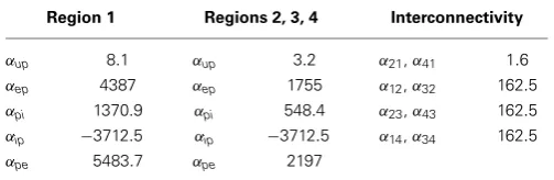
spectral peak at around 10 Hz (alpha activity). The parameter val-ues are shown inTable 4. The accuracy of parameters estimates (connectivity gains) are measured in terms of percentage bias and were taken as the absolute difference between the estimated and true values at the end of each simulation. Simulations were run for 60 s for the single-region model and 100 s for the four-region model, as the parameter estimates were observed to converge well within this time. For state tracking, only the results of the post-synaptic potentials are shown, although the derivatives of the post-synaptic potentials were also tracked. State accuracy was measured by the root mean squared (RMS) error over 1 s of data, since the states (and their estimates) are dynamic. The RMS error was measured from the final second of the simulation, when parameter estimates were assumed to be constant. Results are also presented for a single realization for both the single and four region models (normal and epileptiform) in order to illustrate the convergence properties over time of the parameter estimates. The parameters used to simulate the epileptic-type behavior seen in the simulated seizure transition are given inTable 5. The bounds that were used to constrain the parameter estimates are shown in Table 3.

3. RESULTS

3.1. COMPARISON OF ANALYTIC MEAN AND UNSCENTED TRANSFORM

The performance of the modified Kalman filter and the unscented Kalman filter were compared in order to quantify the increase in estimation performance from using the analytic mean. Both methods approximated the covariance of the joint distribution using the unscented transform. Since the mean and covari-ance cannot be considered separately when the distribution is propagated through the neural population model, the Kalman filter that uses the analytic mean is really an approximation of a Gaussian distribution. However, the difference between the standard UKF and this novel application of the Kalman fil-ter, which is tailored to the neural population model, is that

Table 3 | Parameter constraints used in the clipping method of the estimation algorithm.

Parameter Lower bound Upper bound

αup 0 300

αep,αpi,αpe 0 20,000

αip −40,000 0

αjk,αkj 0 5000

Table 4 | Connectivity parameters to simulate an alpha rhythm in the multi-region population model.

Parameter Value Parameter Value

αup 3.2 α21,α41 76

αep 1755 α12,α32 63

αpi 548.4 α23,α43 44

αip −3712.5 α14,α34 70

αpe 2197

the new approach based on the analytic mean has the poten-tial to improve state and parameter estimation for this particular application.

Tables 6, 7 show the mean estimation bias for intra-connectivity gains and post-synaptic potentials (PSPs) of a single cortical region. Table 6 demonstrates that the analytic mean approach is approximately twice as accurate as the UKF for state tracking ofvup,vpiandvipand has equal accuracy with the UKF forvepandvpe. This is consistent with the parameter estimates in Table 7, which shows that the analytic mean method gave two to three times improved accuracy over the UKF forαup,αpiandαip (and has the same accuracy forαepandαpe).Figure 3shows the results for the entire Monte Carlo simulation and again demon-strates that the Kalman filter using an analytic mean outperforms the UKF for the single region model.Figures 3A,Bshow that the intra-connectivity gain estimation is within 60% for all parame-ters for the UKF and less than 25% for the analytic mean method.

Table 5 | Connectivity parameters used to simulate epileptic behavior in the multi-region population model.

Region 1 Regions 2, 3, 4 Interconnectivity

αup 8.1 αup 3.2 α21,α41 1.6

αep 4387 αep 1755 α12,α32 162.5

αpi 1370.9 αpi 548.4 α23,α43 162.5

αip −3712.5 αip −3712.5 α14,α34 162.5

αpe 5483.7 αpe 2197

Table 6 | Mean bias (over 50 simulations) of the post-synaptic potential estimates for a single region model of alpha rhythms, with comparison between the UKF and the new modified Kalman filter.

Post-synaptic potential RMS Bias (mV)

Unscented transform Analytic mean

vup 0.57 0.32

vep 0.26 0.24

vpi 0.47 0.16

vip 0.58 0.31

vpe 0.30 0.29

Table 7 | Mean bias (over 50 simulations) of the connectivity gain estimates for a single region model of alpha-type rhythms, with comparison between the UKF and the new modified Kalman filter.

Connectivity gain Bias (%)

Unscented transform Analytic mean

αup 7.33 3.45

αep 1.07 1.05

αpi 13.29 4.01

αip 24.01 7.69

FIGURE 3 | Comparison of the estimation results from the modified Kalman filter with the unscented Kalman filter from the Monte-Carlo simulation (50 realizations). (A)The bias for parameter estimation as a percentage of the true value for the connectivity gain using the UKF.(B)

The bias for parameter estimation as a percentage of the true value for the connectivity gain using the analytic mean.(C)RMS error for state tracking of the post synaptic potentials using the UKF.(D)RMS error for state tracking of the post synaptic potentials using the analytic mean. The center line of the box plots shows the median error and the box covers are the 25th to 75th percentiles. The whiskers cover the entire range of errors that are not considered outliers, which are shown by the dots. The outliers are determined to be outsideq1−1.5(q3−q1) toq3+1.5(q3−q1) whereq1 andq3denote the 25th and 75th percentiles.

Figures 3C,D show that the bias for tracking of PSPs is consis-tently less than 1.4 mV for the UKF and less than 0.7 mV for the analytic mean approach. On the whole, these results demonstrate the value of the novel application of the modified Kalman filter for the neural population model.

3.2. SINGLE REGION MODEL

Figure 4shows an example of state tracking and parameter esti-mation for a single cortical region. The plots show that the algorithm was able to reliably track all postsynaptic potentials and estimate all connectivity gains in the region. This remarkable result was achieved using only the noisy ECoG signal and knowl-edge of the structure of the cortical circuit.Figure 4also shows that the standard deviation of the estimated parameters also con-verged, which demonstrates the filter was performing as expected. The standard deviation of the estimate forαip remained larger than the estimates for the other connectivity gains, as it had the largest bounds representing greater uncertainty.

Figures 3B,Dshow the results for parameter estimation and state tracking using the Kalman filter with the analytic mean for a Monte Carlo simulation with 50 realizations. Both fig-ures demonstrate good accordance for estimation results to the actual states and parameters, with the possible exception of the

FIGURE 4 | Estimation results showing convergence of parameters in the single region model.30 s of ECoG data simulating an alpha rhythm from a single region model was used. Each panel shows the PSP (upper) and connectivity gain (lower) estimates. The actual states are shown in red and the estimated values are shown in black. The gray shaded regions show the estimated standard deviation estimates of the connectivity gains. The scale in the lower left of each subpanel is distinct for the PSP (LHS) and connectivity gain (RHS)(A)PSP and connectivity gain for spiny stellate to pyramidal connection.(B)PSP and connectivity gain for pyramidal to inhibitory interneuron connection.(C)PSP and connectivity gain for pyramidal to spiny stellate connection.(D)PSP and connectivity gain for inhibitory interneuron to pyramidal connection.(E)PSP and connectivity gain for external input to pyramidal connection.

inhibitory-to-pyramidal connectivity gain estimate (αip) when using the standard unscented Kalman filter.

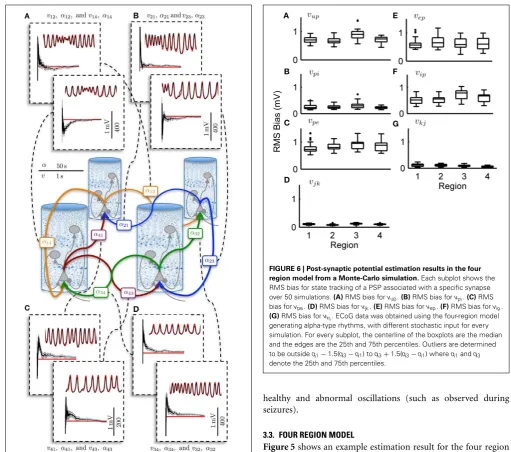
FIGURE 5 | Post-synaptic potential and connectivity gain estimation results for the four region model showing parameter convergence.

ECoG data was obtained over a 50 s simulation using the four region model to generate alpha-type rhythms. The filter output for PSP tracking is over a short time segment and the connectivity gain estimation is for the entire simulation. The actual states are shown in red and the filter output is shown in black. The gray bar around the plot of the connectivity gain estimates shows the standard deviation of the estimate.(A)PSP and interconnectivity gains from region one to two (upper) and four (lower).(B)

PSP and interconnectivity gains from region two to one (upper) and three (lower).(C)PSP and interconnectivity gains from region four to one (upper) and four to three (lower).(D)PSP and interconnectivity gains from region three to four (upper) and three to two (lower).

bias for all of the connectivity coefficients (slow states) was less than 22% with a mean of less than than 8%. It is anticipated that this level of accuracy in state estimation will provide a strong basis for a classification algorithm that distinguishes between

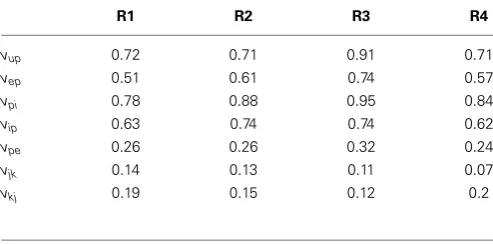
FIGURE 6 | Post-synaptic potential estimation results in the four region model from a Monte-Carlo simulation.Each subplot shows the RMS bias for state tracking of a PSP associated with a specific synapse over 50 simulations.(A)RMS bias forvup.(B)RMS bias forvpi.(C)RMS

bias forvpe.(D)RMS bias forvjk.(E)RMS bias forvep.(F)RMS bias forvip.

(G)RMS bias forvkj. ECoG data was obtained using the four-region model

generating alpha-type rhythms, with different stochastic input for every simulation. For every subplot, the centerline of the boxplots are the median and the edges are the 25th and 75th percentiles. Outliers are determined to be outsideq1−1.5(q3−q1) toq3+1.5(q3−q1) whereq1andq3 denote the 25th and 75th percentiles.

healthy and abnormal oscillations (such as observed during seizures).

3.3. FOUR REGION MODEL

Figure 5shows an example estimation result for the four region model. The four region model has four times as many measure-ments that are inputs to the filter, as there are additional ECoG voltage signals (one per region). However, the dimensionality of the system is more than four times larger than the single column, as each new column introduces an equal number of intra-regional connections as well as two inter-regional connections with its neighbors. In Figure 5, only the inter-regional connections are shown, although all of the PSPs and connectivity gains were esti-mated. The results that are presented inFigure 5demonstrate that the estimation method was capable of scaling up from a single region model to a larger model of coupled regions, while main-taining the ability to simultaneously estimate all the connectivity gains and track the PSPs associated with every synapse. The ability to scale up to a larger area is crucial in order to apply estimation to patient-specific models of epilepsy.

FIGURE 7 | Connectivity estimation results in the four region model from a Monte-Carlo simulation.Each subplot shows the estimation bias as a percentage of the true value for the connectivity gain for every synapse over 50 simulations.(A)Bias forαup.(B)Bias forαpi.(C)Bias forαpe.(D)

Bias forαjk.(E)Bias forαep.(F)Bias forαip.(G)Bias forαkj. ECoG data was

obtained using the four-region model generating alpha-type rhythms, with different stochastic input for every simulation. For every subplot, the centerline of the boxplots are the median and the edges are the 25th and 75th percentile. Outliers are determined to be outsideq1−1.5(q3−q1) to q3+1.5(q3−q1) whereq1andq3denote the 25th and 75th percentiles.

generated sequence foru(t) as external input.Tables 8,9 summa-rize the mean (over the 50 simulations) values of the estimation biases for both fast and slow states.Figure 6andTable 8show that the RMS bias for PSP tracking was consistently less than 1.5 mV and the mean RMS bias was less than 1 mV for all connections. The amplitude of the PSP signals was on the order of 10–30 mV and the variance of noise added to the ECoG voltages was 1 mV. Therefore, the bias for PSP tracking represents a high level of accuracy. As was seen for the single region model, the tracking performance was less accurate forvupdue to the stochastic input that generates this PSP.

Figure 7andTable 9show that the estimation bias for the con-nectivity gains was less than 40% and the mean bias was less than 10%, except forαipandαjkwhich were less than 15%. The param-eter estimation accuracy for the coupled model compared with the single region model was comparable in terms of the mean value for all connectivity gains. Over the entire Monte Carlo sim-ulation, the estimation performance for αep, αpi and αpe were similar to the single region model. The decrease in performance is most evident forαip(from within 20% to within 40%). This is consistent with the results from the single region model whereαip was the least accurate of the estimated gains. The estimation per-formance forαjkandαkjcannot be compared to the single region model. However, the estimation accuracy of the interconnectivity gains was worse than the intra-region gains (apart fromαip). It

Table 8 | Mean RMS estimation bias (over 50 realizations in mV) for post-synaptic potential tracking in the multi-region model.

R1 R2 R3 R4

vup 0.72 0.71 0.91 0.71

vep 0.51 0.61 0.74 0.57

vpi 0.78 0.88 0.95 0.84

vip 0.63 0.74 0.74 0.62

vpe 0.26 0.26 0.32 0.24

v_jk 0_.14 0_.13 0_.11 0_.07

vkj 0.19 0.15 0.12 0.2

Table 9 | Mean bias (over 50 realizations in %) for connectivity parameter estimates in the multi-region model.

R1 R2 R3 R4

αup 6.11 3.6 7.32 6.15

αep 1.05 1.24 1.35 0.63

αpi 6.87 4.01 6.68 4.91

αip 12.21 7.62 13.02 9.14

αpe 1.94 2.16 2.06 2.58

αjk 7.76 8.28 12.92 8.35

αkj 4.48 4.81 8.01 4.94

is difficult to pinpoint sources of error for this parameter, as all of the estimated states are highly interactive with each other. A potential source of the decreased accuracy forαjkandαkj(as well asαup) is that their values are an order of magnitude smaller than the other estimated connectivity gains, which can lead to numeri-cal problems for the Kalman filter equations. On the whole, the consequences of scaling up the model from a single region to four coupled regions has not resulted in major loss of estimation accuracy.

3.4. SIMULATION OF AN EPILEPTIC SEIZURE

Figure 8 shows a simulated ECoG time series with transitions from a background rhythm to seizure-like oscillations and back. The transitions were achieved in the forward simulation by ramp-ing the amplitude of the excitatory gains of one cortical region (region 1 in Figure 8) and then decreasing them back to their usual values. The values used to generate the seizure-type behav-ior are shown inTable 5. In order to ensure that the seizure-like oscillations would spread from one region to the neighboring regions, the interconnectivity between the first area (where the seizure was initiated) to its neighbors was increased from the pre-vious example over the entire time course of the simulation, while the interconnectivity gains from all other regions back to the first region were decreased (as shown inTable 5).

FIGURE 8 | Simulation of an epileptiform transition.ECoG signals were obtained using a 100 s forward simulation and adjusting the connectivity gains from alpha to seizure rhythms and vice versa (seeTables 4,5). The simulation output shows the epileptiform activity rapidly spreading from Region 1 (where the pathology was simulated), to the rest of the network. The figure also shows a graphical representation of the model of the differential measurement function. The blue and red sub-panels show example alpha and seizure-type rhythms, respectively.

covariance to capture unmodeled transitions in parameter val-ues. It is clear that the method has successfully identified the transitions in the cortical region that led to the seizure gen-eration, as the filter tracked the increase in these gains for region 1, while accurately estimating the corresponding con-nectivity gains for the other cortical regions that remained constant.

It can be seen fromFigure 9A that the estimation accuracy forαup was lower than the other connectivity gains due to the stochastic input. The estimated interconnectivity gains that were associated with inputs to region 1 (the epileptic region),α21and α41, also do not quite converge (Figures 9F,G) the actual

val-ues. This could be due to the much smaller magnitude of these gains compared with the corresponding interconnectivity gains

FIGURE 9 | Results from tracking pathological changes in the connectivity gains that lead to epileptiform activity.In each subplot, the red line shows the actual values.(A–G)Show the estimation results from Region 1, where the internal excitatory connectivity gains were transiently increased to induce the epileptiform discharge. The mean is shown by the black line and the gray shaded area shows the standard deviation of the estimate.(H–N)Show the estimates from the non-pathological regions (no change in parameters from baseline), where the solid lines show the mean and shaded regions show the standard deviation of the parameters.

larger amplitude oscillations. If this method of estimation can be translated for use on real data, it has the potential to provide valu-able insight into the cause and spread of seizures and envalu-able more informed treatment measures for epilepsy patients.

4. DISCUSSION

This paper presented a framework for model inversion that facil-itates estimation and imaging of the physiological properties of the brain using electrocorticography (ECoG) data , under the assumption that the model captures the key features of the corti-cal circuits of interest. Tracking of the mean membrane potentials of the various neural populations and connectivity parameters (within and between cortical regions) may provide a clear pic-ture of the causal relationships between cortical dynamics and seizures. The link between physiological parameters and data will undoubtedly improve detection and treatment outcomes across a range of pathologies.

We have demonstrated that is possible to reliably track the post-synaptic potentials and estimate the connectivity parame-ters of a large-scale neural population model. This demonstration highlights the power of combining the prior information we have about neural dynamics and cortical structure (that is encoded in the computational model) to estimate the parameters of interest. For the single region case, the average prediction bias for connec-tivity parameters is less than 8% and the average RMS error in the mean post-synaptic potential estimates within the local cir-cuit was less than 0.4 mV (the peak to peak potential of a typical post-synaptic potential was approximately 20 mV). We demon-strated that the framework can be scaled up to a larger-scale model (of four cortical regions) with more realistic measure-ments without a major decrease in estimation accuracy. The average estimation error remained less than 10% except for three parameters (errors inαip,αjk, andαkjwere less than 15%). The tracking of post-synaptic potentials in the four-region model had mean RMS error of less than 1 mV. Importantly, we demonstrated the ability to track slow changes in the connectivity parame-ters, that led to transitions to and from seizures. Traditionally, functional neuroimaging methods have been very successful, but limited to determining where and when seizures occur. This new method can be used with ECoG data to also determine the mecha-nisms. This knowledge will provide opportunities to develop new therapies.

Traditionally, amplitude, frequency and phase correlations in neuroimaging data have been used as features to study connectiv-ity. While these techniques imply a causal relationship, they can be misleading. For instance, correlations that arise between multiple microelectrode neural recordings could be the result of neurons independently responding to a common stimulus or could be caused by synaptic coupling between neural populations (Friston, 1994). Other possibilities that need to be taken into account are neural populations receiving a common modulatory input from another unobserved region of the brain, or indirect cou-pling between neural populations where connectivity is affected via multiple regions (Friston, 1994). Questions about the sources of correlation in neural recordings are difficult to disambiguate without resorting to more invasive methods of measurement. On the other hand, computational models can directly infer cortical

connectivity patterns and neural dynamics from data, providing the probable cause of empirical observations. The degree to which such causal relationships correspond to the true state of the cortex is limited by the model uncertainty, just as correlations iden-tified using other types of neuroimaging are limited by spatial and/or temporal resolution constraints. However, model uncer-tainty can be quantified, which is a highly useful property for many classification applications.

Under a Gaussian assumption, the Kalman filter provides esti-mates of the probability distributions of the states and parameters of the population model, which is updated as new measurements become available. If the Gaussian assumption holds, the Kalman filter provides the minimum variance estimate of the states and parameters (Simon, 2006). However, the nonlinearities in the model lead to non-Gaussian states. Nevertheless, the Gaussian approximation leads to good estimation results, as demonstrated by the Monte Carlo simulations. However, these results do not guarantee that the state and parameter estimates will not eventu-ally diverge from the actual values, given a measurement times series of a longer duration. This is due to the approximations of the unscented transform. Possible improvements in the esti-mation results could come from using sequential Monte Carlo (SMC) filtering methods, when the Gaussian assumption can be relaxed. However, SMC methods impose a much larger com-putation burden that may make them prohibitive for imaging large-scale neural systems.

The derivation of the analytic a-priori (prediction through the model) state and parameter estimates provided in this paper gives an exact solution for the expected value for a Gaussian trans-formed by a sigmoid, regardless of the shape of the resultant distribution. This improves on the the unscented or extended Kalman filters, which have previously been used in a similar con-text (Voss et al., 2004; Schiff and Sauer, 2008; Liu and Gao, 2013). The Gaussian approximation of the uncertainty in the state and parameter estimates that are predicted by the model is maintained in our framework using the unscented transform.

The implementation of the unscented transform with large covariance matrices is a well established limitation of the filter (Wan and Van Der Merwe, 2000; Simon, 2006; Särkkä, 2013). While scaling up the size of the model did not significantly increase the estimation bias in this case, it does exponentially increase the computation time to the point where it becomes impractical for real-time applications. For increasing numbers of variables to be estimated, the covariance matrix eventually becomes so large that the use of the unscented transform becomes computationally infeasible. The extended Kalman filter is one possible alternative for approximating the covariance, but esti-mation accuracy is compromised (for the sigmoid nonlinearity). A possible direction of future research is improved methods of covariance estimation.

the most appropriate candidate using an information theoretic criterion (Daunizeau et al., 2009). DCM has been applied across a range of data from fMRI (David et al., 2008), ECoG time series (David, 2007) and EEG spectral response (Moran et al., 2008), as well as different phenomena such as seizure prediction (Aarabi and He, 2013) and auditory habituation (Wang and Knösche, 2013). A possible advantage of the Kalman (and sequential) fil-tering approaches over the DCM framework and other similar methods (such as genetic algorithms) is the ability to track slowly changing parameters in real time, which is likely to be particu-larly important when investigating transitions observed in data, such as epileptic seizures.

The algorithm presented in this paper utilized known con-straints of physiological variables. Enforcing concon-straints on states and parameters greatly improved the convergence properties of the filter. Without any bounds applied to the distributions of parameter estimates, the results typically did not converge to a steady value within the simulation time-frame. There are a num-ber of alternative and more theoretically rigorous approaches for constraining the parameter estimates. However, most constraint methods add a significant computational burden to the filter (Simon, 2006; Kandepu et al., 2008), rendering them impracti-cal for implementation in large-simpracti-cale systems. The large number of states and parameters to be estimated restricted the constraint method to clipping, which is computationally efficient to imple-ment. Future work in this area should be to investigate effect of constraints on the estimation performance (such as the estimate variance).

The initialization of the filter, in particular the covariance matrix, is a notoriously inexact science (Wan and Nelson, 1997; Wan and Van Der Merwe, 2000; Simon, 2006; Schiff, 2012). In practice, significant tuning is often required to achieve sta-ble and accurate estimation results. For this study, the initial covariance was based on knowledge obtained from forward sim-ulations. A larger initial covariance was used when the number of hidden variables was increased. The initial uncertainty for param-eters was increased by broadening the range of the constraints. Furthermore, when parameters to be estimated are dynamic rather than static (as would be the case for most parameters of interest in neural models), an additional constant error term is added to the covariance matrix to prevent an overestimate of confidence in the model (Voss et al., 2004). In this case it was found that additional uncertainty should be very small relative to the magnitude of the parameter. The amplitude of the addi-tive uncertainty is analogous to a learning rate parameter in other algorithms. It can be relatively easily tuned by examining the convergence rate the parameters (i.e., seeFigure 9).

The estimation framework presented in this paper can be nat-urally integrated with other existing imaging technologies and computational methods in the field of neuroscience. All methods of neuroimaging are essentially inversion problems, that rely on a transformation from the measurement space to the source space. An example is the transformation of magnetic radiation to the haemodynamic response in fMRI. Typically, measurements are transformed using a specific inversion technique to determine the state of the neural tissue. The framework presented in this paper applies the same philosophy. However, the transformation from

the measurement to the source space is via a generative model. The generative model reflects the current state-of-the-art of our knowledge of the mesoscopic biophysics and anatomy of cortical circuits. By the same token, limitations and uncertainties in our current knowledge can also be quantified and incorporated into the model, making all predictions reflect probability distributions rather than scalar values. The mapping from neural population models to measurements can be readily adapted to describe dif-ferent modalities, via alternative observation equations, enabling multiple sources of data to be combined to form a unifying model. The difficulty of measuring brain activity in a minimally invasive manner makes it imperative to use as much informa-tion as possible to predict neural states and inter-connectivities. A framework that combines patient-specific measurements with well accepted principles of brain structure and function, and importantly, knowledge of uncertainty, is an important step toward the lofty goal of reverse engineering the brain.

The estimation framework presented in this model could be used as the first stage of a seizure prediction system, providing the necessary features that are used as inputs to a classifier. It is neces-sary to represent neural data using representative features in order to reduce the dimensionality of the problem prior to applying a classification algorithm. In the past, efforts have focused on defin-ing features that are correlated with ictal and pre-ictal periods and, as such, can be used in a predictive capacity (Andrzejak et al., 2001; Lehnertz et al., 2003). Recently a patient-specific seizure classifier for ECoG was implemented using parameters identified from a neural mass model (Aarabi and He, 2013). The advan-tages of using neural states and parameters as features for seizure classification is that they are naturally patient-specific (since they are directly relatable to the neural activity) and may also provide clues as to the underlying cause of seizures, which could inform treatment strategies.

The capability of neural models to be tailored to an individ-ual patient’s data is particularly relevant to the investigation and treatment of epilepsy, since it is a highly patient-specific disorder. The mechanisms for seizure onset and propagation vary signifi-cantly between patients (Wendling et al., 2005; Mormann et al., 2007; Coombes and Terry, 2012). Ideally, information about neu-ral interconnectivity should be obtained on a case-by-case basis using an individualized model (Blenkinsop et al., 2012; Nevado-Holgado et al., 2012). A reliable model inversion framework will enable more precise targeting of therapies. The information provided by a model-based framework could also predict the response to drug treatments or electrical stimulation in a simu-lated environment, sparing a patient the negative side effects that may arise from a trial-and-error approach. Models can also be used to provide feedback for deep brain stimulators for robust prevention of seizures (Mormann et al., 2007; Adhikari et al., 2009).