Rochester Institute of Technology
RIT Scholar Works
Theses
Thesis/Dissertation Collections
10-1-1993
A Self-timed implementation of the bi-way sorter
systolic array processor
Mitchell Diamond
Follow this and additional works at:
http://scholarworks.rit.edu/theses
This Thesis is brought to you for free and open access by the Thesis/Dissertation Collections at RIT Scholar Works. It has been accepted for inclusion
in Theses by an authorized administrator of RIT Scholar Works. For more information, please contact
Recommended Citation
A Self-Timed Implementation of the Bi-Way Sorter
Systolic Array Processor
by
Mitchell S. Diamond
A Thesis Submitted
ill
Partial Fulfilhnent of the
Requirements for the Degree of
MASTER OF SCIENCE
ill
Computer Engineering
Approved by:
Graduate Advisor - Prof. George A. Brown
Department Chair - Dr. Roy Czernikowski
Reader - Dr. Tony Chang
DEPARTMENT OF COMPUTER ENGINEERING
COLLEGE OF ENGINEERING
ROCHESTER INSTITUTE OF TECHNOLOGY
ROCHESTER, NEW YORK
THESIS RELEASE PERMISSION FORM
ROCHESTER INSTITUTE
OF
TECHNOLOGY
COLLEGE OF ENGINEERING
Title
of
Thesis:
A Self-Timed Implementation
of
the
Bi-Way
Sorter Systolic
Array
Processor.
I,
Mitchell
S.
Diamond,
hereby
grant
permissionto
the
Wallace
Memorial
Library
of
RIT
to
reproduce
my
thesis
in
wholeor
in
part.
Signature:
Abstract
Self-timed
circuits
withan appropriate
handshake
controlcircuit can
be
usedto
replace
the
global clock
in
a
VLSI
chip.
By
replacing
the
global clock
many
problems
which
face
designers
have
disappeared along
withthe
clock.
Some
of
these
problemsare
due
to
clock skew and
capacitance
scaling
withsmaller
feature
sizes.
The
wirecapacitance
cannot
scale
below
a
certain
limit due
to
two-dimensional
effects,
therefore
the
RC
delays
associated
withthe
interconnect
layers
do
not
scale
proportion.ally
to the
feature
size.
The
resultant
increase in
wiredelay
makes
it
difficult
to
distribute
a global clock at a
high frequency.
This
project
takes
anexisting
synchronous systolic
array, the
bi-way
sorter,
and
implements
the
sorteralgorithm
using
a self-timed approach.
By
using
self-timed
instead
of
synchronous
approaches,
many
ofthe
problems
associated
withsynchronous
circuits
suchas
clockskew and
large line
capacitance,
are avoided.
In
this
thesis,
a
2-bit,
four
numbersorter
willbe designed
and
simulated
and
the
Table
of
Contents
1.0 Introduction
1
1.1
What is Self-timed?
1
1.2
Self-Timed
vs.Synchronous Circuits
2
2.0
Theory
ofthe
Bi-Way
Sorter Algorithm
andthe
Handshake
Controller Circuit
6
2.1 The
Bi-Way
systolic
sorting
algorithm6
2.2 The
Self-Timed
Circuit
13
2.2.1 The
Self-Timed
Logic Operator
13
2.2.2 The
Handshake
Control Circuit
(HCC)
16
3.0 Implementation
ofthe
Bi-Way
Sorter Cell
20
3.1 VHDL
Overview
20
3.2 The Sequential
Bi-Way
Sorter
21
3.2.1 The VHDL Model
ofthe
Sequential
Bi-way
Sorter Cell
23
3.2.2 The Transistor Model
ofthe
Sequential
Bi-way
Sorter Cell
27
3.3 Implementation
ofthe
Self-timed Sorter Cell
32
3.3.1 The VHDL Model
ofthe
Self-timed Sorter Cell
33
3.3.2 The
Transistor Model
ofthe
Self-timed Sorter
cell35
3.3.3 The Layout
ofthe
Self-timed
Sorter
cell43
4.0 Implementation
ofthe
Handshake Controller Circuit
(HCC)
46
4.1 Implementation
46
4.1.1 VHDL
modelofthe
Handshake
Controller
Circuit
48
4.1.2 The Transistor
modeloftheHandshake Controller
Circuit
51
4.1.3 The Layout
ofthe
Handshake Controller
Circuit
58
5.0 A Self-timed Four 2 bit Number Sorter
Array
60
5.1
Overview
of aSystolic
j\rrayProcessor
60
5.2 Description
ofthe
Self-timed Sorter
Anay
Processor
61
Table
of
Contents (Continued^
5.2.1 Data
Dependencies Between Cells
in
the
Array
61
5.2.2 Operation
ofthe
Self-timed
Bi-way
Sorter
Array
63
5.3 Simulaton
results ofthe
self-timed
bi-way
sorter67
6.0 Conclusion
70
Appendix A
Example
ofSorting
four 2-bit
numbers
using
the
Synchronous
Bi-way
sorterarray
processor
A-l
Appendix B
Circuits
and simulationfor
the
latch
andthe
mutiplexor usedin
the
synchronousbi-way
sorterB-l
Appendix C
Quine-McCluskey
methodfor
sorterlogic implementation
C-l
Appendix D
VHDL
codefor
the
number generator module andthe
b
control signal moduleD-l
Appendix E
Schematic
and simulation of componentsin
the
self-timed sorter moduleE-l
List
of
Figures
Figure 1.1
Diagram
ofthe
contributions which effectthe
driving
capcity
ofthe
clocksignal
3
Figure
2.1 Diagram
of abi-way
cell7
Figure 2.2 3x2
array
ofbi-way
cells10
Figure 2.3 DCVSL logic
withready
signal15
Figure 2.4a Petri-net
describing
the
operation ofthe
HCC
19
Figure
2.4b
Logic diagram
ofthe
interconnection
between logic
modules19
Figure 3.1 Circuit
ofthe
sequentialbi way
cell22
Figure 3.2 VHDL Code for Sequential
bi-way
sorter24
Figure 3.3 Simulation
ofthe
sequentialVHDL
codefor
the
bi-way
sorter26
Figure 3.4
Schematic
ofthe
synchronous sorter module28
Figure 3.5
Schematic
for
me
control module withinthe
bi-way
cell29
Figure 3.6 Simulation
andtiming
resultsfor
the
control gate circuit30
Figure
3.7
Simulation
ofthe
synchronous sorter cell31
Figure 3.8 VHDL
programfor
the
Self-timed
Bi-Way
Sorter
cell34
Figure
3.9 Schematic for
the
Self-timed
sorter cell36
Figure 3.10 Schematic
ofthe
regular nmostree
37
Figure 3.11 Schematic
ofthe
inverse
nmostree
38
Figure 3.12 Schematic
ofthe
ready
signal generator circuit40
Figure 3.13 Simulation
ofthe
ready
signal circuit41
Figure
3.14 Simulation
ofthe
one-way
cell42
Figure
3.15 Layout
ofthe
bi-way
sortercell45
Figure
4.1
Modified handshake
controllercircuit47
Figure 4.2 VHDL
codedescribing
the
Handshake Controller Circuit
49
Figure
4.3 Logic Diagram
ofthe
HCC
50
List
of
FiguresfContinueri^
Figure 4.4
Simulation
ofthe Handshake
Controller
Circuit
52
Figure
4.5 Schematic
ofthe
Handshake
Controller
Circuit
53
Figure
4.6
Test
Circuit
usedto
determine
timing
characteristics
ofthe HCC
56
Figure
4.7 Simulation
ofthe
test
circuit
for
the
Handshake Controller
Circuit
57
Figure
4. 8
Layout
of theHandshake
Controller
Circuit
59
Figure 5.1 Example
ofthe
self-timedarray
processor62
Figure 5.2
Schematic
ofthe
self-timed
bi-way
sorter processor64
Figure 5.3 Operation flow
ofthe
Self-timed
Bi-way
Sorter
66
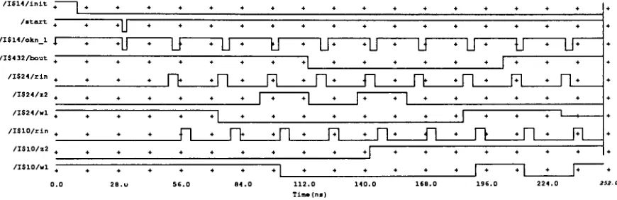
Figure 5.4 Simulation
waveforms
ofthe
selftimed
sorter processor69
Figure Al Example
ofsorting four 2-bit
numbersusing
the
Synchronous
Bi-way
sorter processor
A-3
Figure
Cl Karnough
maps usedto
reducethe
logic
equationsfor
the
nmostrees
C-5
Figure Dl Generator
module usedto
generatethe
unsortednumbersD-2
List
of
Tables
Table 1.1
Selection
of x andy based
onthe
b
input
9
Table
3.1 Truth
table
describing
operation ofthe
oneway
cell33
Table
4.1
Timing
determined from
the
HCC
simulation55
Table 5.1 Simulation
resultsfor
the
self-timedbi-way
sorter68
Table
Cl
Quine-McCluskey
reductionC-2
Table C2
Quine-McCluskey
reductionC-2
Table
C3
Quine-McCluskey
reductionD-3
Table C4
Quine-McCluskey
reductionD-3
GLOSSARY
VLSI
IC
RC
MSB
LSB
HCC
VHDL
DCVSL
Bi-way
sorter
Handshake Controller
Self-Timed
Very
Large Scale
Integrated
circuit
Integrated Circuit
Resistor-Capacitor
Most Significant
Bit
Least
Significant
Bit
Handshake Control Circuit
Very
high
speed
integrated
circuit
Hardware
Description Language
Differential Cascode Voltage Switch Logic
A dedicated high
speed
sorter processorModule
Controlling
data swapping between
modules
A design
where
the
control over
the
activity in
the
system
is distributed
overthe
components
that
compose1.
Introduction
1.1
What is
Self-Timed?
The
operation
of a
synchronous
system
is
reminiscent of marchers
moving
uniformly
to the
beat
of
the
drum in
a
parade.
The
temporal
controls of
the
marchers
are
centralized
in
a single
"authority",
and
the
marchers
respond
by doing
their
tasks
in
synchronism
withthe
marching
cadence.
This
type
ofcontrol results
in
a simple
form
of
organization
whichpeople
seem
to
associate
withthe
efficiency
of
machines.
However,
this
rigid
behavior is
not
the
only way
to
coordinate
these
tasks,
nor
is it
efficient unless all
the tasks
are
very
wellmatched.
Self-timed
systems
use a
different
approach
to
managing
the tasks that
have
to
be
performed.
This
method allows
eachsystem module
to
have
some
control overwhen
it does its
tasks
while still
conforming
to the
overall operation of
the
system.
A
designer
must assure
that
all systemtasks
occur
in
a
propersequence,
but nothing
everhas
to
occur at a particular
time.
Self-timed
circuits
are
categorized
as
a
cross
between
synchronous
and
asynchronous
circuits.
The
self-timed
methodology
more
closely
resembles
the
asynchronous circuit.
A
synchronous circuit
usesa
global clockthat
controls
the
operation of
the circuit;
every
module reacts
to
the
clockpulse at
the
same
time.
An
asynchronous
systemdoes
not usea
clock andthe
control ofthe
circuitis usually
sporadic and
does
not appear
to
be rigidly
organized.
The
self-timed concept arose
from
asynchronousinterfaces
usedat
the
board
level.
The
term
"self-timed"indicates
that
the
circuit
doesn't
usea global
clock,
instead it functions
through
data dependencies between
modules.
A
module starts
the
other
modules
via an
asynchronous communication circuit
known
as
the
Handshaking
Control Circuit (HCC).
Self-timed
circuits eliminate
the
problem of
delays
caused
by
logic
elements
and
interconnects,
placing
more
emphasis
on
individual
element
design.
This
is
the
central
idea
of
self-timed systems:
each system
"part"controls
its
time
of operation.
1.2
Self-Timed
vs.
Synchronous Circuits
The
mainreason
for
the
use
ofself-timed
circuits
is
that the
synchronous
approach
becomes less
suitable
for
present
integrated
circuit
(IC) technology
and
willbecome
even
less
appropriate
withfuture
technology.
The
total
chip
area
for
most
designs
has
remained
constant
orin
some cases
has increased
as
the
feature
size
has
been
reduced.
This
has
allowed
the
number of active on
chip
devices
(transistors)
to
increase dramatically.
Therefore
although
the
gate
capacitance
of
the
individual
transistors
has
been
reduced
withthe
feature
size, the
increase in
the
number ofdevices
being
driven
by
the
system
clockhas increased
the
total
capacitance
load
onthe
clock
driver.
Synchronous
technology
is
hindering
IC
miniaturizationby increasing
the
driving
capabilities needed
for
a clock
driver
circuit.
To
illustrate
this point,
consider a
global clock
which willdrive
a wire
witha number of
transistors
(N)
attached
to
it. In
this
example some assumptions
willbe
made.
It
willbe
assumed
that the
wire
is
made
of one
type
of metal and
that
each
transistor
along
the
wire
has
the
same
dimensions.
A diagram
of
the
circuit and
the
variables
being
used
are shown
in figure 1.1.
To find
the total
delay
of
the
clock
signalbased
on
the
examplecircuit
wehave
to
find
the
capacitance
and
the
resistance of
the
wire and
the transistors.
Equations
1, 2,
and
3
show
the
equations needed
to
find
the
capacitanceand
the
resistance
ofeach element
of
the
circuit.
The
approximate
total
delay
canbe
determined using
the
resistance
equation
for
the
total
delay
of
the
circuit
is found
by
substituting
equations
1
,2
and
3
into
the
delay
equation
whichis
shown
in
Eq. 4.
To
analyze
the
effect
of smaller
feature
sizes
upon
the
delay
equation,
the
effects
of each variable
willbe
examined.
The
sheet resistance
(Rsheet)
f
the
w^e
wiUremain constant
due
to the
nature
ofthe
metal.
The
same applies
to the
permutivity
constants
eu^e
and eox.
The
area of
the
IC
willstay
constant
whichmeans
the
interconnects
of
the
wires
willremainabout
the
same
length
(0.
The length
(L)
and
width(W)
of
the transistors
willdecrease in
size.
The
spacing
between
the
metal and
the
poly
(d^g)
will remainthe
same
due
to the
fabrication
technology.
The
thin
oxide
(Xox)
of
the
gate
willdecrease
withthe
feature
size.
By
examining
the
total
contributions
of eachvariable, the
overalldelay
willbe
reduced
slightly
withthe
decreasing
feature
size.
But
the
new affects
imposed
on
the
delay
of
the
clock signal
willincrease dramatically. The
total
gate
driving
capacitance
with
the
newfeature
size
will willbe
muchlarger
than
withthe
smallerfeature
sizes
because
there
are
many
more
transistors
onthe
line contributing
to the total
delay
ofthe
clock signal.
clocl^
<r
>
Cg Cg Cg
A
<
*
.N
Metal
r
Cg
Cwire
at.
I
Poly
^
^
Figure 1.1 Diagram
ofthe
contributions which effectthe
driving
capacity
of_
eA
_eLW
(--gate-v ~ v(1).
Aox
Aox
C
_eUneA
_line
^
,-. '"wire-,,
(^).
"-Vine
"line
/?
=PT
=f-=i?
7
(3).
X
=R\C
+NC
1
-Rsheete-line
l
.
M?,to
e0x^
L l
,as"to
AA
Another
problem
that
effects
the
useof
future IC
technology
is
the
problem
of clock skew.
Clock
skew
complicates
the
problem of
distributing
the
clock signalto
all parts of
the
circuit at
the
same
time.
If IC feature
size
keeps getting
smaller and
the
total
design
area gets
larger,
the
ability
to
drive
the
increased
capacitance
of
the
circuit,
caused
by
clocksignal
distribution,
willbecome
close
to
impossible. Designers
today
are
trying
to
overcome
the
problem of clock skew
by
introducing
specific
delays
into
their
circuits
to
compensate
for
the
non-synchronousbehavior.
Two
methods
ofaccomplishing
this
is
either position each module onthe
chip in
a
certainplace
to
create a
delay
or
introduce
delay
buffers into
the
circuit.
This
cannot continue
for
long
if
the
industry
desires
to
increase
clock
frequency
because
circuits
wouldhave
to
be
redesigned
to
compensatefor
the
delay
which was changedin
the
origionalcircuit.
Until
now, the
asynchronous approachhas
not
been
popularbecause
of circuit
overhead,
design
difficulty,
and
poor performancebecause
of
the
added
delay
of
managing data
flow
through
the
system.With
the
advance
of
technology
these
obstacles
may be
overcome.
The
extra area
neededfor
handshaking
controllers
is less
of a
penalty
now
because
of
smallerfeature
sizes of
IC
chips.
Also,
withfaster IC
technology
the
overheaddue
to
these
handshaking
controllersbecomes
nominal.
maximum
feasible
system clock speed
is determined
by
gate
delays.
Thus,
the
self-timed
approach
willbecome
a more
attractive approach
for IC designers
whenIC
circuits can operate
beyond
the
maximum
feasible
global
systemclock speed.
The
optimal
performances of self-timed circuits are
determined
by
the
speed
that
data
can
be
transferred
between
modules and
the
speed
with whichthe
HCC's
can accomplish2.0
Theory
of
the
Bi-Way
Sorter Algorithm
and
the
Handshake
Controller Circuit
2.1
The
Bi-Way
systolic
sorting
algorithm
Sorting
is
one of
the
most
frequent
tasks that
a computer performs.
In
order
for
humans
to
understandand
coordinate
large
amounts
of
data,
there
must
be
some
order
to the
data.
Applications
whichrequire
sorting include
such
diverse
tasks
as
database
management, graphics,
and
weather
forecasting.
Sometimes
a
general
purpose
processorwould
not suffice
for
some
applications,
so a
dedicated
processoris
needed.
The
bi-way
sorter
is
one such processor.
The
bi-way
sorterprocessor
wasfirst
proposed
in
a
paper entitled"Bi-way
Sorter:
a
Two-Dimensional
Systolic Array"[l].
The
objective
wasto
modify
anexisting sorting
processorand
increase
its
speed
whiledecreasing
its
area.
The
bi-way
sorter
is
a synchronous systolic
array
composed
of modules
called
"bi-way
cells."
Each
bi-way
cellis
made
up
of
one-way
cells
by
multiplexing between
the
bottom
set
of signals
(zl
and
w2)
and
the
top
set
ofsignals
(z2
and wl).The
bi-way
cells are
interconnected in
an
array
structure.
By
exchanging
commands,
data
flow is directed
through
the
array.
In Figure
2. 1
there
is
a
diagram
ofthe
bi-way
cellshowing
the
connections ofthe
inputs
and outputs
to the
cell.
Each
cellhas
to
make
a
decision
depending
onthe
value
of
the
bit
stored
in
the
celland
the
new
bit coming into
the
cell.
Two
controlsignals
rand s
determine
the
comparisondecision:
no
decisions,
storethe
incoming
number,
or
bypass
the
incoming
number.There is
also a
b
controlline
that
controls
which
inputs
are
directed
into
the
cell.The
b input
also
controlsthe
flow
ofdata in
wl
11
/\
zl
>^bFA]/
3
3
one-way
cell
\l/
z2
J,
w2
Figure 2. 1 Diagram
ofa
bi-way
cell
The
one
way
cell
takes
data
inputs
xy,
control
inputs
rs,
and
outputs signals
u,v,r',s'.The
bi-way
cell usesthe
b
input
to
multiplex
the
wl,z2 or w2,zlsignals
into
the
xand
y
inputs
of
the
one
way
cell.
The
wland
w2signals are
the
uand
vsignals
The one-way
cell
takes
four
inputs r,s,x,y
and
produces outputs
r',s',u,v.
To
direct
either
the
top
or
the
bottom
signals
of
the
bi-way
cell
into
the
one-way
ceU's
inputs
x,y, the
b
input is
used
based
on
the
values
in Table 2.1.
The
heart
ofthe
bi-way
sorter
is
the
method of
choosing
whichinputs
are
encountered
by
the
one
way
cell.
If
the
b
input is
low
then
xand
y
willtake
on
the
input
from
the
top
zland
it
willoutput
to the
bottom
w2respectively.
If
the
b
input
is
high
then
xand
y
willtake
onthe
input
from
the
bottom
z2and
it
willoutput
to
the
top
wlrespectively.
Once
the
specific
xand
y
values are chosen
the
one-way
cellsteers one of
the two
bits
corresponding
to the
smaller
number, to the
uoutput and
passes
the
larger bit
to the
voutput.
The
r*and
s'
lines
indicate
the
result
ofthe
comparison:
(r',s')=(0,0)
for
no
decision, (r',s')=(l,0)
to
switch
xand
y (or
store
the
incoming
bit)
and
(r',s')=(0,l)
to
not switch
xand
y (or let
the
incoming
bit bypass
the
cell).
By
only using
one-way
cells,
numbers
can
only be
sorted
in
one
direction
through the
array.
This
means
that the
amount of cells required
is
equalto the
product
of
the
size
ofthe
array
to
be
sortedand
the
bit-size
of
the
array
elements.
The
bi-way
cell algorithm was
derived
to
cut
the
number ofrequired cells
in half
whilestill
sorting
a
data
set of
the
same size.
This
is
accomplished
by letting
the
numbers
flow
into
the
array
then
back
out
ofthe
array in
the
opposite
direction, hence,
doubling
the
numberof comparisons
whichcan
be handled
by
the
smaller array.Another
feature
ofthe
bi-way
sorter
is
that
it
can sort numbers
in
two
directions.
This
is
accomplished
by
letting
data flow
eitherin
from
the
bottom
ortop,
depending
onthe
order required.
If
the
data flows in from
the
top
the
data
willbe
sortedfrom largest
to
smallest.
If
the
data flows in
from
the
bottom
the
data
willbe
sorted
from
smallest
to
largest.
By
b
data
flow
stored num Xy
0
up
largest
zl w21
down
smallest wl z2*
As
sy
7yT
1
1
S
_^.
/N
\jX
w
*
1
}
MSB
LSB
*
^
}
_^.
/N
sy
TT
Figure 2.2. 3x2
.arrayof
bi-way
cells
The
array
can
be increased
in
size
by
adding
modules
as shown
by
At every
clock
pulsethe
data flows into
each cell and
is
compared
withthe
bit
already
stored
in
that
cell.
The
cell
makes
a
decision based
on
the
bit coming in
and
the
stored
bit.
One
of
three
decisions
can
be
made: allow
the
bit
to
pass
through the array,
hold
the
bit
and send
the
previously
stored
bit
to the
next
cell,
or no
decision.
The bit
is
stored
in
the
cell
by
using feedback
on
the
uand
voutputs.
By
repeating
this
process
each
bit
is
compared
withall
the
other
bits
in its
column.
The
first
column of
the
array is
composed
ofcontrol cells.
These
cells
do
not
have data
pass
through
them,
rather
they
send out control signals
r',s',b'that
control
the
sorting
process of
the
rest of
the
array.
Data
flows
from
top
to
bottom
or
from
bottom
to
top
depending
on
the
b
input,
and control signals
flow from left
to
right.
The data is
sent
into
the
array in
a
skewed-bit-paralleldata
format
wherethe
MSB
is
one clock cycle ahead of
the
next most significant
bit
and so on.
A
skewed-bit-parallel data format is described
as
having
the
MSB entering
the
cells
followed
by
the
next
bit
place one
clocktick
later
and so
on until you reachthe
LSB. The
skewed
data format
allows
eachbit
ofa
numberto
arrive
at
the
bit-comparison
cell
in
its
column at
the
same
time
as
the
comparisondecision
from
the
nextmost
significant cellin
that
row.
Below
is
an example
if
a set
oftwo-bit
data
valuesand
the
conversionto
a
skewed-bit-parallelformat.
Set
of numbers
Skewed-bit-parallel
format
00
Ox
01
00
10
11
11
10
xl
Example
ofa
conversionto
skewed-bit-parallelformat
The
number of cells needed
in
the
array is based
ontwo
variables:The
number
of
data
values
to
be
sorted.
The
number of
bits
needed
to
represent
each
data
value.
The array
is
set
up in
the
following
fashion.
The
left
hand
column
is
made
up
of
the
control modules.
The
next column
.andsubsequent
columns are needed
depending
on
the
number of
bits.
The
number of rows needed
is
equalto the
total
numberof
data
values
divided
by
two.
By
using
this
formula
expansion
is
easily done.
For
example,
to
set
up
a
aneight
bit
twenty
data
valuearray
you wouldneed nine
columns and
ten
2.2 The Self
Timed
Circuit
The
Self-timed
circuit
is
composed
of
two
parts:
1
.The logic
operator
which
performs
a
specific
task.
2. The
Handshaking
Controller
that
controls
the
data
transfer
between
logic
operators.
2.2.1 The
Self-Timed
Logic
Operator
The
logic
operator
is
a
module
that
evaluates
a
particular
function.
The
difference between
a
synchronous
and a self-timed
logic
operator
is
the
productionof
a
ready
signal.
Synchronous
circuits
all run on a global clock.
The
global clock
is
set
up
witha period equal
to the
slowest
module
in
the
system.
Operators
have
a
rigidly
defined
number
of
periods
necessary
to
evaluate
their
function.
With
self-timed
operators
no
global
clock
is
used.This
means
that there
has
to
be
a
different
mechanism
set
up
to
accommodate
the
operator's evaluation
delay.
A
mechanismmust
be devised
whichindicates
to
the
controller
whenthe
evaluationhas been
completed.
This
mechanismis
called
the
ready
signal.
There
are
many
ways
of
generating
the
ready
signal.
The
following
two
methods are examined
to
demonstrate
two
popularextremes.
One way is
to
artificially
mimic
the
delay
of
the
logic
operator.
This
is
done
by
inserting
a
delay
element
withinthe
logic
module
that
willsend out
a
ready
signal
based
on
the
maximumtime
needed
to
evaluate
the
function.
By
creating
the
ready
signalthis way,
weare
reverting
to the
synchronous
methodology
whichslows
down
the
operationof
the
system
based
ona
maximum
delay
time.
This
approachis
unacceptableand cannot
be
considered
in
a
self-timed
design
because it does
not allow
the
logic
module
to
operate at
its
own
speed.
Once
the
operator's
task
is
complete
it
should
indicate
this
to the
controller.
Another
method,
which
is
more
acceptable,
generates
a natural
ready
signal.
This
signal
is
created
whenthe
logic
operator
has
completed
its
task
and not after an
artificial
delay.
One
convenient
way
to
produce
the
natural
ready
signal
is
to
implement
the
logic
operator
with
a
dynamic differential logic family.
The
most
popular
circuit
is
the
DCVSL
(Differential Cascode
Voltage
Switch Logic).
Figure
2.3
shows
a
diagram
of a
DCVSL logic
operator.
There
are
two
important
properties
of
domino
DCVSL
that
lends
this type
of
circuit
to the
implementation
of
the
self-timed
logic
operator.
One property is
that the
circuit
is
free
of
delay
hazards[2].
A
circuit
is
said
to
have
delay
hazards
if
the
output
depends
on
the
relative
delay
ofthe
signal
paththrough the
logic.
This is
detrimental because
a
false
output might register as a
completion
that
will set off
the
ready
signal
prematurely.
DCVSL logic is free
of
delay
hazards because
the
design is
organized
to
prevent
feedback
from
other
logic
modules
being
used
to
produce
the
final
output answer.
Another
property
that
is
important
to the
stability
of
the
ready
signal
is
the
case
of race states.
The logic
module
has
to
be
designed
in
such a
way
as
to
not
let
race
states
occur.
This may be
accomplished
through
the
use
oflogic
circuits
in
a
precharge-evaluate
scheme.
In
the
precharge
state, the
outputs
ofthe
logic
structure
are switched
to their
high-voltage
states.
When
the
circuit goes
into
the
evaluation
phase
the
outputs are
then
free
to
assume
their
logical
valuedetermined
by
two
nmos
pull-down
trees.
If
the
nmos
trees
are
duals
ofone
another, the
output of one
tree
willbe
high
and
the
other
low
during
the
evaluationphase
producing
the
output signal and
its
complement.
By
using
this
method
a
transition
canonly
occur
from
"11"(i.e.
charging
phase)
to
either
"10"or
"01".
There
can never
be
a
conditionwhere
both
the
output
signal and
its
complement
willchange
state,
suchas(ex
"ll"->
"00"
or
"00" ->VDD
START
Inputs
/
READY
Figure 2.3
DCVSL
logic
withready
signalThe
ready
signal
is
generatedby
logical
ORing
the
output
and
it's
complementtogether.
Since only
one output
willchange
there
cannot
be
a race
state
in
the
system.
Because
of
these
special
properties,
a
reliable
ready
signal can
easily be derived
from
the
output
terminals
of
the
domino DCVSL.
This
is
done be creating
a
ready
signal generator circuit which
checks
to
see
if
the
output
function
and
its inverse
are
different
values.
If
this
occurs
the
answer must
be
validand
the
ready
signal goes
high.
While in
the
precharge phase
both
outputs are
"1"so
the
ready
signal canonly
produce a
"0"as
its
output.
The
unpopularity
of
the
asynchronous
approachin
the
past
was
caused
primarily
by
the
extra
hardware
circuitry
required
for
the
generation ofthe
ready
signal.
At
that time
domino DCVSL logic did
not exist.
The design
of
hazard-free
asynchronous circuits
involved
adding
redundant states
into
the
logic
that tended to
make
the
overall circuit
muchlarger.
Also,
creating
the
inputs
neededfor
the
logic
was
more
difficult
to
implement
than
a
global clockcircuit.
Logic
was slow relative
to
an
easily
obtainable clock
frequency
and
the
circuit overhead was
substantialin
size
and
performance.Now
the
technology
exists
to
make self-timed circuits a more
viablesolution.
2.2.2 The Handshake Control
Circuit
(HCC)
The
Handshaking
controlleris
the
heart
ofany
self-timed system.Its job
is
to
control
the
logic
operator's evaluationof
the
incoming
data,
and also
to
synchronize
the
passing
of
data from
one
moduleto
another.The
HCC
musthave
the
following
propertiesif
it is
to
performits job
as
fast
and as
flawlessly
as
possible.One property
whichis
associated withthe
HCC
is its
modules.
Since
in
a
self-timed circuit
every
module
is evaluating
at
different times,
any
one
module
has
no
knowledge
of when
it
must
begin
its
evaluation.
The HCC
must
be
small and
execute
its
task
with great speed.
The
time
for
the
HCC
to
execute
the transfer
of
data
should
be less
than the time
it
takes
for
the
logic
operator
to
evaluate
its function.
If
this
were not
so, then the
HCC
would
add a
delay
to the
operation
ofthe
circuit
and
the
asynchronous
self-timed
approach wouldbe
counterproductive.
For
this
reason great care must
be
taken
in
the
design
ofthe
HCC
to
maximize
speed.
The HCC
uses
the
ready
signalinformation
to
control
the
transfer
ofdata
between
the
logic
operators.
A
4-cycle
handshaking
protocol
is
suitable
whenemploying
domino DCVSL.
In 4-cycle
handshaking,
for
eachrequest signal sent out
by
the
HCC
there
is
an
acknowledge
signal
whichfollows
it.
Data
is
validonly
while
the
ready
signal
is
active.
The handshake
signals are
usually
called
REQuest
and
ACKnowledge.
A
ready
signal generated
by
a self-timed
logic
operatorindicates
to
the
HCC
that the
operatoris
finished
doing
its
computations.
This
causes
the
HCC
to
signal
the
next operator
to
performa
data
transfer.
When
the transfer
is
done,
the
controller
whichsent
the
REQ
signal
willreceive
an
ACK
signalfrom
the
next
controller.
Once
received
the
controller willstart
the
computation cycle
overagain.
In Figure
2.4a
there
is
a
diagram in
the
form
ofa
petri net andin Figure 2.4b
there
is
a
logical
model
diagram
describing
the
workingsof
the
HCC.
In
orderfor
data
to
be
validfrom
the
previous module
three
signals must
be
set.First,
the
previous
module
has
to
set
its
REQuest
out
signalto
indicate
to the
present module
that
it
is
finished
withits
computation(Pl).
Second,
the
present modulehas
to
be done
withits
previous computations
(P3)
and
finally
the
next
modulemust
have
accepted
the
newly
computed
data
from
the
present module(P5). Once
the
above
occurs, the
new
data
is
latched
(Tl)
and
anACKnowledge
signalis
sentto the
previous module(P2)
and a
new
computationcan
nowbegin
(T2).
When
the
present moduleis done
withits
computation,
a
REQuest
out signal
is
sent
to the
next
HCC (P4).
The
cycle
willthen
KEY
Pl: REQin
P2: ACKout
P3:
computationdone
P4: REQout
P5: ACKin
Tl: latch
data
T2:
processdata
Figure 2.4a
Petri-net
describing
the
operation of
the
HCC
<r
self-timed
logicoperator
-%
_^k
HCC(n-l)
If
input
data(n)
outputdata(n)
I
self-timedlogicoperator
rout(n
F
REQi;
5f
ACKout
self-timed
logicoperator
ready(n)
J<
REQout
HCC(n)
K
*
ACKin
-^
HCC(n+l)
K-Figure
2.4b Logic diagram
of
the
interconnection between
logic
modules
3.0
Implementation
of
the
Bi-Way
Sorter Cell
3.1 VHDL
Overview
The
one-way
cell was
first
implemented
using
the
VHDL
(Very
High
speed
integrated
circuit
Hardware
Description
Language)
programming
language,
whichis
an excellent candidate
for
the
creation and simulation of
hardware
circuit models.
One
reason
for VHDL's popularity is
that the
language
is
able
to
describe
the
hardware
model
at
different design levels.
There
is
the
functional behavioral
model whichsimulates
the
hardware in
a
fashion
much
like
the
C programming language.
Timing
factors
are not
introduced into
this
model and
the
program
describes
the
behavior
ofthe
circuit and not
the
actual
hardware implementation.
The behavioral
modelis
a
good
starting
point
in
designing
a circuit
because
emphasis
is
onthe
properoperation
of
the
systemwithout regard
to the
actual
implementation.
The
next
level
of
complexity
is
the
dataflow
model,
whichsimulates
the
actual
circuit modules and
the
data
that
flows between
them.
The
modelis usually broken up
into
processes.
Each
process
describes
a
module
withinthe
circuit.
In
VHDL,
processes
runconcurrently
thus
simulating hardware
parallelism.Processes
cancommunicate
with eachother
using
objects
called signals.
Signals
can
be described
as
the
wires
between
modules.
Data
flow
models
ordinarily don't involve
timing
concerns
and are
mostly
usedto
verify
that
modules
worktogether.
Finally,
there
is
the
structuralmodel,
whichstrictly
simulates
the
hardware
circuit.
The
structural modelincorporates full
timing
characteristicsof
the
circuit
elements and modules as
wellas a
precisedescription
of
the
interconnects between
modules.
VHDL
aids
hardware designers
by
permitting
them
to
design
and simulate a
VHDL
models
to
be
converted
directly
to
hardware
implementations
using
synthesis
design
automation
tools.
3.2 The
Sequential
Bi-Way
Sorter
The
sequential
one-way
cell was
implemented
using
steering logic.
Steering
logic is
a
methodology
whichcontrols
the
flow
of
the
input bits
through
a
cellto
their
designated
outputs
using
certain control signals.
The flow
ofthe
bits
are controlled
using
multiplexors
and
a
control
module
signal whichselects
the
output
ofa
multiplexor.
The
architecture
ofthe
bi-way
sorter
cellis
shownin Figure 3.1.
The
cell
contains
seveninputs
and
five
outputs
which weredescribed
in
chapter
2.
The
execution of
the
one-way
cell
is
as
follows: First
the
data
inputs
are steered
to
xand
y
depending
on
the
b
control
line.
Then
either
xand
y
or rand s are steered
to
the
r'and
s'outputs,
depending
onthe
output
ofthe
rand
s control module.Finally,
x andy
are either steered straight
through
to
uand v or
they
are switched
depending
onthe
s'
value.
flfiffg
Figure 3.1 Circuit
ofthe
sequentialbi-way
cellThe
cell
is
implemented
using
steering
logic.
The
multiplexors steer
the
inputs
through
the
ceUto
their
3.2.1 The VHDL
Model
of
the
Sequential
Bi-way
Sorter Cell
The
sorter cell was
first
implemented
using
the
VHDL programming language.
The
model
description
usedis
a combination of
the
data flow
and
the
structural modeltypes.
By
using
a combination of
the two models,
components can
be described using
the
data
flow
style while also
incorporating
some aspects
from
the
structural model.By
adding
specific
timing
values
to the
data
flow
modelthe
circuit
canmore
accurately
simulate
the
hardware
whilekeeping
the
code
less
complex than
the
structural modeltype.
The
code was
broken up into
processes
whichdescribe
the
operationof
the
multiplexors and
the
control module.
The
processesare
interconnected using
signaldeclarations.
The
code
for
the
sequentialone-way
sorter canbe found in Figure 3.2.
The
code
was writtenand
compiledusing VHDL
version8.1 from Mentor Graphics
Corporation.
At
the
beginning
of
the
source
code,
library
statements were addedto
load
extra commandlogic
states,
anddata
types
whichare
specificto the
Mentor
software.
The
entity
declaration
follows
the
loading
ofthe
libraries.
The
entity
declaration
specifiesthe
nameof
the
circuitas
wellas
defining
the
input
and
outputports
ofthe
circuit.The
signalsdeclared in
the
port
statement arethe
same signals which werediscussed
in
chapter2.
The data
type
QSIM_STATE
is
a
specialdata
type
usedby
Mentor's
simulators,
and
has four
possible values:the
Z
state
(high
impedance),
the
X
state(indeterminate
value),
1
and0 (logic high
andlogic low).
Each
port
signal was givenan
initial
value of either1
or0.
If
the
ports werenot
initialized
the
simulator woulddefault
valuesto
the
X
state,
causing
the
logic
equations
to
evaluateincorrectly.
--Mitchell Diamond Thesis Project 6/10/93
--This is a structural model of the Sequential
bi-way
sorter cell
--load in
libraries
LIBRARY
mgc_portable, ieee;
USEmgc_portable.qsim_logic.ALL;
USE mgc_portable.qsim_relations.
ALL;
USE ieee.std_logic_1164.
ALL;
ENTITY str_beh_sorter_new IS
PORT
(
Clk: IN OSIM STATE b: IN QSIM STATE r,s: IN QSIM STATE Zl,z2: IN OSIM STATE bp: OUT QSIM STATE rp,sp: OUT OSIM STATEwl,w2: IN QSIM STATE U,V: OUT QSIM_STATE END str_beh_sorter_new;
ARCHITECTURE struct OF str_beh_sorter_new IS
='0 ='0 ='0 ='0 ='0 ='0 ='0 ='1')
SIGNAL X: QSIM STATE ='0 SIGNAL y= QSIM STATE ='0
SIGNAL sptmp: QSIM STATE ='0
SIGNAL Ctl:
QSIM_
.STATE='0BEGIN
bp
<=b;
tmuxl:PROCESS!elk,
b,
zl,w2,wl, z2) BEGINIF clk='l'
THEN IF b '
0' THEN
x<=zl AFTER 0.6 9 ns;
y<=w2 AFTER 0.69 ns; ELSE
x<=wl AFTER 0.69 ns;
y<=z2 AFTER 0.69 ns; END IF;
END IF; END PROCESS muxl ;
mux2:PROCESS
(elk,
ctl,x,r, s,y) BEGINIF clk='l'
THEN IF ctl='0'
THEN
rp<=r AFTER 0.69 ns;
sp<=s AFTER 0.69 ns ; sptmp<=s AFTER 0.69 ns;
rp<=x AFTER 0.69 ns; sp<=y AFTER 0.69 ns; sptmp<=y AFTER 0.69 ns; ELSE
clock input direction control control lines
top
and bot. bitsoutput dir. Ctrl. output control
feedback sigs. stored bits
internal sig.
internal sig.
sel sig mux3.
sel sig for mux2.
--set
bp
signalchoose 0 sel.'
s
--choose 1 sel.
'
s
send r to rp out. send s to sp out. make Ctrl sig.
send x to rp out.
send y to sp out.
make ctl sig.
switch bit. switch bit. --store bit. --store bit. END IF; END IF; END PROCESS mux2 ;
mux3:PROCESS
(elk,
sptmp,x,y)BEGIN
IF elk ='1' THEN IF sptmp '0'
THEN
u<=y AFTER 0.69 ns;
v<=x AFTER 0.69 ns; ELSE
u<=x AFTER 0. 69 ns; v<=y AFTER 0.69 ns; END IF;
END IF; END PROCESS mux3 ;
control:PROCESS
(elk,
r, s,y) BEGINIF clk='l'
THEN
etl<=(not(x) AND not(r) AND not(s)) OR (not(y) AND not(r) AND not(s)) AFTER 1.0 ns;
END IF; END PROCESS control; END struct,
The
.architecturesection
is
where
the
specific model
is formed.
An entity
canhave
multiple architecture's
describing
the circuit,
eachhaving
its
own
modelstyle.
In
the
architecture
body
several
signals are
declared.
The
xand
y
signals represent
the
internal
.signalsof
the
one-way
cell,
the
ctlsignal
is
the
output control
line from
the
control process.
The sptmp
signal
is
used
to
control
the
selection of
the
outputs
in
the
mux3 process and
is derived from
the
s'output
ofthe
mux2process.
The
multiplexor processes all
have
the
same
generalimplementation.
An
IF-THEN
statement
is
used
to
control
whichset
ofinput
signals are
directed
to the
output signals.
In
the
process
declaration,
signals
whichare
used withinthe
process
are
listed in
parentheses
after
the
PROCESS
statement.
This list is
called
the
sensitivity list.
The
simulator will evaluatethe
process
if any
ofthe
signals
have
changed
in
valuein
this
list.
The
elk signalappears
in
eachsensitivity list in
orderto
allow
eachprocess
to
be
evaluatedduring
each clock cycle.The
control process usesa
logic
equation which producesthe
correct
ctl signalbased
onthe
input
signals
x,y,r,s.
Within
the
code,
AFTER
clauses are usedin every
signal assignment.The
AFTER
clauses
notify
the
simulatorto
assignthe
computed value ofthe
signalto
the
output
aftera
fixed time.
The
timing
for
eachclause
wasdetermined from
the
simulation
of
the transistor
implementation
of
the
celland
willbe discussed in
the
next
section.
The VHDL
program wastested
using
the
Quicksim logic
simulatorsoftware
version
8.1 from Mentor Graphics
Corporation.
In Figure 3.3
a
trace
is
found for
the
simulation of
the
bi way
cell
VHDL
code.
To
test
the
cell,
all
combinationof
inputs
(r,s,zl,w2)=(0000
->1011)
were enteredto
the
cell.Output
waveforms arealso
shown.
Figure 3.3 Simulation
ofthe
sequential
VHDL
code
for
the
bi-way
sorter
The
simulationshows
a
test
patternconsisting
of
allcombinations
of
the
inputs
r,s,zl,w2.
The
output
signals
1*
1
A
4*i
4 1* 41
*1
'1
?1
\
I*1
*1
?I
4?1
t
4
1*
1
*1
* /b4 4 4 4 4 4 4 4 4 4
4 4 4 4 4 4 4 4 4 4 4 ?
*l
/r 4;
4 4;
4 4 4 4 4 4
1
1
* 44 4
4
4 4 ? *
1
4 + *
1
4 * 4/il
4
*
1
4 4
{
44
4
4 *
1
i
*i
* 44
1
? ?1
4
I
4 4 /21
* 4 *1
41
4 41
1
* 4*l
\
*4 4 /rp
?1
4 4 4 + 4 4 +(1
4 4 Zap1
* ?1
1
?A
4
4 4
4
4 * 4
*l
4
4
12.0
n* *
n
4i
44 /u r
1
4 4 72.04 ?
1
1
4 4
4 F~ *
1
460.0
i
/v i* ?u
24.u 4 36.04
I
*A
*1
84.u
0.0 48.0
Tin* (ns
96.0 108.C
3.2.2 The Transistor
Model
ofthe
Sequential
Bi-way
Sorter
Cell
The
sequential
sorter cell was
modeled
using
cmos
logic
circuits.
The
sorter
cell
described
in
[Orton,Peppard,Aki,1992]
was
implemented
using
three-micron
technology.
In
this
paperthe
sorter
cell
was
implemented
using
a
two-micron
technology
in
order
to
make
the
comparison
more
consistent
withthe
self-timed
implementation
ofthe
same sorter
cell which wasalso
designed using
a
two-micron
technology.
Figure
3.4
is
a
schematic
diagram
of
the
sorter cell circuit.
The
circuit consists
of
multiplexors,
latches,
and a
controlmodule;
schematics and
timing
results ofthe
multiplexors and
the
latches
can
be found in Appendix B.
A
single
shift-register wasused
as a clocked
latch
to
store
the
output results after
eachclock cycle.
The
controlmodule circuit
is
shownin Figure 3.5.
Equation
1 describes
the
output
signal ofthe
control module.
ctl
=(rVXy'+x')
(1).
A
simulationof
the
controlcircuit
is
shownin Figure
3.6.
The
control circuit wastested
withall
possible valuesof
the
four,
signalinputs (x,y,r,s).
The
ctloutput
waveforms and
the
timing
results are also
shownin
the
simulation.
The
delay
of
the
output
signal wasdetermined
by
taking
the
averagetime
for
the
outputto
evaluate allof
the
input
signals.
The
average
delay
time
was
calculatedto
be 0.42
nanoseconds.The
entire cell was
then
simulated and
tested
for accuracy in evaluating
all
combinations
ofthe
inputs.
The
simulation results canbe found in Figure 3.7.
The
top
set of
waveformsare
the
inputs
to the
cell and
the
bottom
set
ofwave
forms
are
output results of
the
cell.
The
delay
ofthe
cell outputs weremeasured
to
be 2.1
Figure
3.4 Schematic
of
the
synchronous sorter module
The
sorter cell
consists
of nine
inputs
and
five
outputs.
The
transistor
sizing for
eachmodule
werecomputed
depending
on
the
loads
each module
had
to
drive.
The sizing
characteristics
are
shown onthe
schematic.
Q. -O
ll
o 'H
0
CM
Stl o-i
:o-0