Effective SAR image segmentation and sea-ice floe distribution analysis via kernel graph cuts based feature extraction and fusion

Effective SAR Image Segmentation and Sea-Ice Floe Distribution

Anlyssis via Kernel Graph Cuts based Feature Extraction and Fusion

Soumitra Sakhalkar

_{, Jinchang Ren}

_{, Phil Hwang}

_{and Paul Murray}

1_{Centre for Excellence in Signal & Image Processing (CeSIP), Department of Electronic and Electrical Engineering,}

University of Strathclyde, Glasgow, G1 1XQ, UK.

2_{Scottish Association for Marine Science (SAMS), Oban, PA37 1QA, UK.}

{soumitra.sakhalkar, jinchang.ren, paul.murray}@strath.ac.uk, [email protected]

1 RESEARCH PROBLEM

The Sea Ice that grows in the open seas like the Arctic sea, forms varying shapes and size due to the fracturing as well as thickening caused by the strong gale force winds and sea waves. Over the winter season, due to the cooler temperature, these sea-ice regions combine with each other to make a stronger and larger sea ice block. In the summer however, due to the higher temperature, they separate into smaller and weaker floes as shown in Figure 1.

Figure 1: An area of sea ice region captured during the beginning of the month of the early summer period on the left and during the ending in the month on the right.

Sea-Ice monitoring has gained significant interest in recent years, largely due to the fact of the decreasing area and thickness of the older arctic sea ice (Kwok, et al., 2009) (Stroeve, et al., 2008). This decline in older sea ice has been linked largely to the growth of younger, thinner sea ice regions (Maslanik, et al., 2007) and also climate changes (Holloway & Sou, 2002), caused by greenhouse gases (Serreze, et al., 2007).

The study of Polar Regions using Synthetic Aperture Radar [SAR] has been widely used for identification of sea ice floes, their size and their distribution (Burns, et al., 1987) (Rothrock &

Thorndike, 1984), (Soh, et al., 2004), (Soh & Tsatsoulis, 1998). This is because SAR is not majorly affected by the harsh weather conditions or the illumination variations and it is able to cover large and primarly inaccesible areas (Xu, et al., 2014). This is particularly important for ensuring safe marine navigation as well as supporting studies of climate changes, like ours, of the Polar Regions.

To date, the process of developing an automatic algorithm for effective segmentation of SAR Sea-Ice images has not been achievable. As a result, analysis of sea ice images relies on a time consuming expert analysis which is performed manually. For this reason, it is primarily important to develop techniques to automatically segment the sea-ice regions from the background and subsequently extract these sea-ice regions from the SAR image. When this is completed it will become possible to build a Floe Size Distribution (FSD) database, where FSD is a measure of the distribution of the different size of the sea ice floes. An FSD database will be constructed in our project by extracting and storing the total pixel area of these individual sea-ice regions in the SAR image and grouping them according to their size. The result will then be used to generate a graph of the size distribution of the floes on different days in a year of the Arctic region. The outcome of our study will further develop scientist’s understanding of the different trends as well as the various conditions affecting the size of the Arctic sea ice floes for that particular year. Eventually this will improve our understanding of the changes in the sea-ice extent over the year by means of comparison with the past several years’ results.

2 OUTLINE OF OBJECTIVES

The main aim of this study is to create novel techniques to automatically segment and extract the sea ice floes from the SAR images of the area in the Arctic region being monitored. To achieve this it is important to fulfil the following smaller objectives;

1. To develop an optimal segmentation technique for accurately segmenting individual ice floes from the background as well as from each other.

2. To refine the methods developed in 1 so they are efficient and inexpensive to compute. 3. To remove/reduce the speckle noise present in

almost every SAR image using appropriate filters. That is, using filters which retain the original image characteristics as well as removing/reducing the presence of speckle noise.

4. To make the techniques developed completely automatic and dynamic so that they can process any SAR image to segment the ice floes.

The result of completing these objectives will be a robust and efficient global machine learning algorithm for segmentation. Furthermore the algorithm parameters will be computed automatically depending on the image statistics derived from the current image under study. This will introduce a step change in the way the sea ice floes are analysed.

3 STATE OF THE ART

Due to the decrease in sea ice floe extent and thickness, it has become increasingly important to generate a better understanding of the environmental as well as the social impacts on the transformation of Arctic sea ice over the duration of each day in a year.

The need for automated segmentation techniques for ice floe analysis has led to some popular floe related studies: examples include techniques for classification using dynamic thresholding for separation and heuristic geophysical knowledge (Haverkamp, et al., 1995), deformation of sea ice by means of measuring the opening and closing of leads (Fily & Rothrock, 1990) and floe size identifications and measurement (Korsnes, 1993). More recent studies have tried to achieve this by using the two

texture analysis methods, Markov Random Fields (MRF) and Gray-Level Co-occurrence Probabilities (GLCP) (Clausi & Yue, 2004), or by using stochastic ensemble consensus approach (Wong, et al., 2009), utilisation of Bayesian segmentation approach with MRF model (Deng & Clausi, 2005) and using pulse-coupled neural networks (PCNN) (Karvonen, 2004).

Although many of these approaches have been implemented, tested and provided in the literature, they do not meet the necessary criteria for application to our data. This is largely due to the fact that the existing techniques are either data specific and can only be applied to segment sea ice floes in certain parts of the world or they involve manipulation of the data or in other cases take too long to compute. As a result, the currently used approach relies on the lengthy technique of manually segmenting the regions based on expertise and knowledge of a sea-ice expert.

There have also been some automated approaches for Sea-Ice segmentation; using an intelligent system named Advanced Reasoning using Knowledge for Typing Of Sea ice (ARKTOS). ARKTOS automatically segments the regions and generate the descriptors for the segmentation of sea ice floes. Others use expert rules for classification (Soh, et al., 2004) using the analytical tool: Automated sea ice segmentation (ASIS). ASIS uses local thresholding for obtaining and retaining information in the image. Image quantization has also been used to obtain the different classes within an image and computing spatial attributes of each class using Aggregated Population Equalization (APE) concept (Soh & Tsatsoulis, 1998). Nonetheless all these have been deemed unsatisfactory to be used for our study due to the same reasons indicated before.

Recent developments in image segmentation techniques have led to a new approach called Graph Cuts [GC] with kernel mapping which is based on the work of (Salah, et al., 2011). GC is based on energy minimization for effectively finding a cut {segmentation} between regions (Boykov, et al., 2001). GC have been used in many studies for image segmentation, for instance in (Rother, et al., 2004), an iterative and interactive GC based approach has been used for effective foreground extraction, whereas in (Boykov & Funka-Lea, 2006) & (Boykov, et al., 2001) GC is used for segmenting the regions using image histogram analysis.

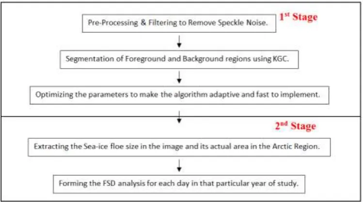
Figure 2: Methodology of our study.

(Zhu & Yuille, 1996), Active Contours (Caselles, et al., 1997) (Chan & Vese, 2001) and Level Set using Mumford and Shah model (Vese & Chan, 2002).

Also in many studies like (Muller, et al., 2001), (Scholkopf, et al., 1999), (Dhillon, et al., 2007), (Schölkopf, et al., 1998), (Girolami, 2002) and (Zhang & Chen, 2002), the so called kernel trick has been used for effective and efficient clustering of complex data.

Similarly many studies have used Kernel mapped Graph cuts (KGC) for image segmentation, examples include spine image fusion to replace CT and MR (Miles, et al., 2013), for classification of brain images (Harini & Chandrasekar, 2012), for segmentation of abdomen MR images (Luo, et al., 2013), for segmentation for MR images with intensity inhomogeneity correction (Luo, et al., 2013).

Thus it can be seen how Kernel mapped Graph Cuts, have until now, been mostly used for medical image processing as opposed to SAR sea ice image processing like our study. In fact, to the author’s knowledge KGC based techniques have not yet been used to segment images containing ice floes. It is therefore proposed that a technique using GC will be applied to automatically segment ice floes in SAR imagery. To deal with the speckle noise, we also propose the addition of an effective pre-processing and image filtering stage which will lead to an optimal segmentation result.

4 METHODOLOGY

The entire processing procedure for our study is shown by the flow chart given in the Figure 2. As seen in Figure 2, the methodology for our study is split in two major stages;

1. This will involve segmentation of sea ice floe using the existing KGC algorithm. It will also incorporate our proposed contribution of the addition of a pre-processing stage to improve the results and a technique to allow the optimization of the parameters which will make the algorithm adapt automatically for processing the image under study.

2. On completion of Stage 1, the next step will involve the extraction of individual sea ice floes to build the FSD analysis for each image for each day in that particular year of study.

We will now briefly explain the existing algorithm; KGC and then explain the importance of our contribution to the algorithm for the improvement of results.

4.1 The Kernel Graph Cuts

et. al. (Salah, et al., 2011), who initially proposed this technique. This algorithm is based on a three stage processing procedure;

1. K-means clustering to find the initial clusters and their centroids.

2. Kernel mapping of the image into higher dimensional feature space.

3. Image Segmentation achieved using Graph Cuts.

4.1.1 K-means based Clustering

K-means is a popular un-supervised and easy to implement clustering method, first introduced by Lloyd (Lloyd, 1982). In fact a survey of clustering algorithm some years ago showed how K-means, even after 25 years was still the most widely used clustering algorithm (Berkhin, 2002) at that time.

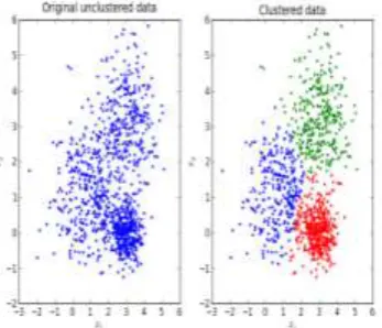
The algorithm partitions/clusters a given set of data into k clusters depending on the least squared distance of each point from that cluster’s centroid. K-means is an iterative process, which continually estimates the least squared distance from the cluster centroid and re-assigns the data into these ‘k’ clusters until the process is stabilized. An example of a set of data points clustered into 3 clusters represented by the three different colours for each one, is illustrated in Figure 3.

Figure 3: K-means based clustering example.

4.1.2 Kernel Mapping

Kernel mapping or the kernel trick is a popular technique used in many recent image segmentation

algorithms (Muller, et al., 2001), (Scholkopf, et al., 1999), (Dhillon, et al., 2007), (Schölkopf, et al., 1998), (Girolami, 2002) , where a kernel function is used to map a data set into a higher dimensional feature space, so that partition of regions is possible.

Figure 4, first seen in (Salah, et al., 2011), illustrates how the kernel mapping aids a better and faster separation /segmentation of result, due to the implicit mapping of data set into higher dimensional space, so that the GC algorithm can be applied.

Figure 4: Illustration of a non-linear data separation. Data separation is non-linear in data space. The data is mapped into a higher dimensional feature space using a kernel. The separation is now linear in feature space, separated by a hyper plane.

There are many popular kernel functions commonly used in the field of digital image processing; examples include the Gaussian/ radial basis function kernel, polynomial kernel, sigmoid kernel and many more as mentioned in (Genton, 2002).

For our study, we will use the Gaussian/ radial basis function (RBF) (Buhmann, 2003) kernel, due to its simplicity and ease of implementation, for mapping into higher dimensional feature space. The equation for the RBF kernel is given by,

𝐾(𝑦, 𝑧) = 𝑒𝑥𝑝 (−‖𝑦 – 𝑧‖

2

𝜎2 ) (1)

4.1.3 Graph cut based Image Segmentation

based on the minimization of the two energy terms given by,

E(f) = ESmooth(𝑓) + EData(𝑓) (2)

Here, ESmooth is the Smoothness cost which

measures the extent to which a label f is no longer piecewise constant and EData is the Data cost which

measures the disagreement of the current labelling f

with the observed data. The labelling f mentioned here is assigned by the K-means clustering algorithm in the initial stage of the KGC algorithm. A labelling f is said to be piecewise constant if it varies smoothly on the surface of the object but changes dramatically at the object boundaries.

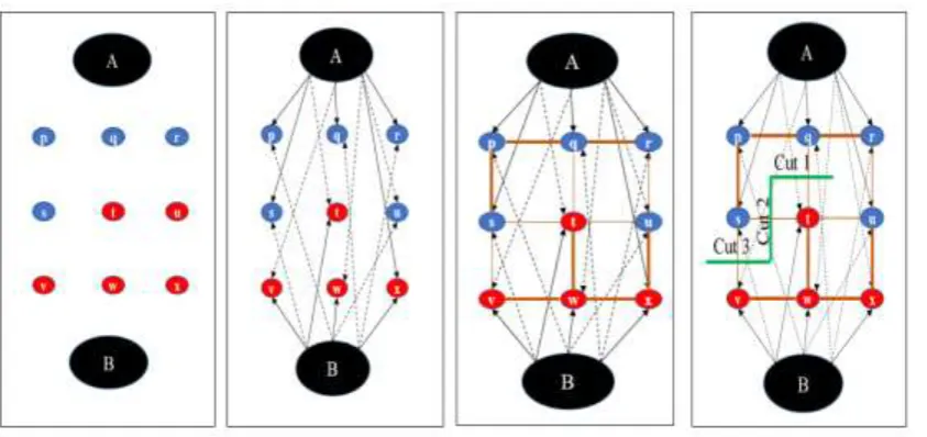
Figure 7 shows the step-by-step procedure of how a GC algorithm finds a cut {segmentation}. Figure 7(a) shows the initial labelling for the pixels before loading the graph for the GC algorithm; blue pixels (p - s) belong to label A and red pixels (t - x) belong to label B. In Figure 7(b) the GC algorithm then assigns the labelling and weights of each pixel with each of the labels A and B using the Data cost term. The darker arrows denote the more likelihood of a label being assigned to a pixel, while the dotted arrow denotes low likelihood of a label being assigned to a pixel. It can be seen how the pixel u is now indicated to be more likely to present label A. In Figure 7(c) the weights of each pixel with its neighbouring pixel are then assigned using the Smoothness cost term. Similar to the previous section, the darker lines denote the more likelihood and the weaker lines show less likelihood of a pixel being associated to be similar to each other. In Figure 7(d) the GC algorithm finds a cut between the labelling one neighbouring pixel pair at a time. It can be seen how the GC now assigns pixel u to label

A based on the most likelihood (Data Cost) and similarity measure (Smoothness Cost).

4.1.4 Drawbacks

Although the KGC algorithm has various advantages over the conventional image segmentation techniques, it still has limited number of drawbacks which need to be addressed to make the image segmentation more robust and efficient.

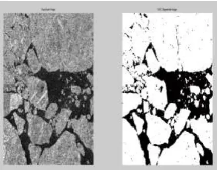
Figure 5 shows an area where the KGC works really well and produces really good results and in Figure 6, it can be seen how the KGC produces very poor results due to the heavy presence of speckle noise in that region of the original SAR image.

Figure 5: One example result of the KGC segmentation.

Figure 6: Other example result of the KGC segmentation.

4.2 Pre Processing

For our study, we propose the addition of a two stage pre-processing routine to help improve the performance of the existing KGC based segmentation algorithm. This pre-processing step involves filtering the image using adaptive filters to remove the speckle noise before applying morphological processing. The aim is to improve the classification result from the K-means and subsequently the segmentation result from the KGC algorithm by first applying these pre-processing techniques.

4.2.1 Adaptive Filtering

Figure 7: Step-by-Step procedure of GC algorithm finding a cut using min cut-max flow algorithm.

Hence for this purpose we have used the Adaptive Median (AM) filter (Qiu, et al., 2004), which uses the local statistics within a filter window to mark a pixel as speckle noise and remove/reduce this speckle noise present in the image. We have compared our results with other popular speckle filtering techniques like the Lee filter (Lee, 1980) (Lee, 1981), Frost filter (Frost, et al., 1982) (Frost, et al., 1981), Bilateral filter (Tomasi, 1998), Median filter & Wiener filter (Lim, 1990), Local Sigma filter (Eliason & McEwen, 1990) and found that the AM filter to be the most suitable for our study. For the scope of this paper, we have not added the comparison results.

4.2.2 Morphological Processing

Other popular techniques, widely used for pre and post processing are the morphological filters such as dilation and erosion (Matheron, 1975) (Serra, 1982) (Dougherty & Lotufo, 2003). In terms of image processing, Dilation, enlarges the image features based upon the size and shape of the structuring element chosen. Erosion shrinks the image features and can also remove them based upon the size and shape of the structuring element chosen. The

morphological processing is extensively explained extensively in (Gonzalez, et al., 2004). For the purpose of our study we have used morphological closing, which is a dilation followed by an erosion using the same structuring element.

For our study, we have used morphological processing to overcome the aforementioned drawbacks of the KGC algorithm and produce better K-means clustering results.

For this purpose, we build a mask image, by thresholding the original grayscale image using standard deviation. We use standard deviation rather than grey level threshold for thresholding to make the process more adaptive to the current image under study.

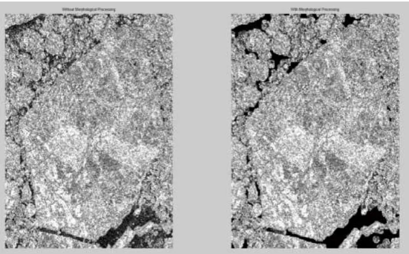
This is then followed by our addition of morphological processing. We then multiply this mask image with the original grayscale image to produce a morphologically enhanced image as seen in Figure 8.

Figure 8: Morphological processing on the KGC segmentation result

5 EXPECTED OUTCOME

It is anticipated that a major outcome of this study will be a novel, fast and reliable algorithm for sea ice floe image segmentation. The algorithm will be easy to use so that environmental experts are able to replace the current manual analysis with this sophisticated and robust technique.

Beyond this, the outcome of this work will help us develop our understanding of the environmental as well as social factors affecting the Arctic Sea ice floe cover. For this, a detailed analysis of sea ice floe needs to be done, with the implementation of the FSD analysis. This will be done to monitor the sea ice floe extent on each day of subsequent year.

This data will then be compared with the results of the FSD analysis done in the same area in the Arctic Region from the previous years and will then help us validate the theory that the older Arctic sea ice floes are indeed getting reduced and replaced by younger, weaker sea ice floes.

Beyond this it is also anticipated that this study can be applied to a wide range of applications. Some examples would include segmenting medical images of a biological nature or microscopic images of metals and other similar materials. Our addition of

the adaptive filtering process can also be used for other noise removal applications.

6 STAGE OF THE RESEARCH

6.1 Results

We now present our results by means of a comparison between the results produced with the original KGC algorithm and the results produced as a result of our addition of the proposed pre-processing stage. To validate the efficacy of the proposed approach, real SAR images with a high resolution of 16k by 16k have been used for both visual assessment and quantitative analysis.

The algorithm is coded in Matlab running on a Dell Inspiron 5537 laptop with 2.3 GHz processor, 4 GB RAM and 64 bit Windows 8.1 operating system. It requires approximately 41 minutes for obtaining the segmentation result for the entire 16k by 16k original SAR image. The processing speed can be further optimised and reduced to run even faster, but it is currently not the main area of focus of our study.

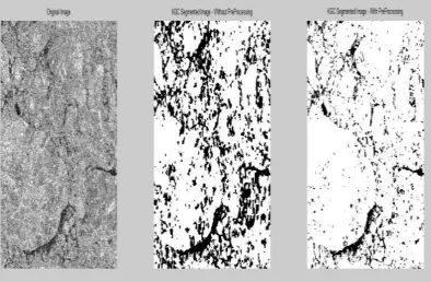
Figure 9: Comparison Result on Image 1.

our addition of a pre-processing stage. It can be seen how our addition improves the segmentation result of the five sample sub sections of the main 16k by 16k real SAR Sea-Ice image, visually.

6.2 Progress to Date

We have now met the first 3 objectives of our study. These involved selecting a fast, accurate and adaptive algorithm for segmenting the sea ice floes and refining the algorithm to make it more efficient.

These can be verified from the descriptions of the KGC algorithm in the previous sections and as evidently seen in Figures 9 & 10. Figures 9 & 10 portray how our proposed pre-processing stage, removes/reduces the speckle noise present in the SAR images and validates how our addition improves the KGC segmented results for the SAR sea ice images.

6.3 Future Work

We now need to focus on extracting the floe size information of these segmented sea ice floes. In order to achieve this, it is first necessary to further separate the floe regions which are not currently separated in some regions but which can be visually predicted to be separated. For achieving this, we are currently implementing another popular energy based image segmentation algorithm; Active Contours (Caselles, et al., 1997) or also referred to as “snakes”. Active Contours currently being used for our study are based on the algorithm developed by Chan & Vese (Chan & Vese, 2001).

The active contour is although known to be notoriously slow due to the large number of iterations required to achieve a good segmentation. To reduce this processing time, we are currently also building an adaptive algorithm to only extract the regions where separations of sea ice floe need to be implemented as per our visual perception. We have been able to achieve some minor improvements but more work needs to be done in order to achieve the optimal results for the extraction of these sea ice floe regions.

ACKNOWLEDGEMENTS

We would like to thank Scottish Association for Marine Science (SAMS) and NERC for providing us with such a challenging and interesting topic for our study and for their funding support "NE/L012707/1"

and "NE/M00600x/1" to make this study possible. We would also like to thank the University of Strathclyde for their motivation and support for conducting this study.

REFERENCES

Berkhin, P., 2002. A survey of clustering data mining techniques, San Jose, CA: Accrue Software.

Boykov, Y. & Funka-Lea, G., 2006. Graph cuts and efficient ND image segmentation. International journal of computer vision, 70(2), pp. 109-131. Boykov, Y., Veksler, O. & Zabih, R., 2001. Fast

approximate energy minimization via graph cuts.

IEEE Transactions on Pattern Analysis and Machine Intelligence, 23(11), pp. 1222-1239. Buhmann, M. D., 2003. Radial basis functions:

theory and implementations. Cambridge: Cambridge university press.

Burns, B. A. et al., 1987. Multisensor comparison of ice concentration estimates in the marginal ice zone. Journal of Geophysical Research: Oceans (1978–2012), 92(C7), pp. 6843-6856.

Caselles, V., Kimmel, R. & Sapiro, G., 1997. Geodesic active contours. International journal of computer vision, 22(1), pp. 61-79.

Chan, T. F. & Vese, L. A., 2001. Active contours without edges. IEEE transactions on Image processing, 10(2), pp. 266-277.

Clausi, D. A. & Yue, B., 2004. Comparing Cooccurrence Probabilities and Markov Random Fields for Texture Analysis of SAR Sea Ice Imagery. IEEE Transactions on Geoscience and Remote Sensing, 42(1), pp. 215-228.

Deng, H. & Clausi, D. A., 2005. Unsupervised segmentation of synthetic aperture radar sea ice imagery using a novel Markov random field model. IEEE Transactions on Geoscience and Remote Sensing, 43(3), pp. 528-538.

Dhillon, I. S., Guan, Y. & Kulis, B., 2007. Weighted Graph Cuts without Eigenvectors:A Multilevel Approach. IEEE Transactions on Pattern Analysis and Machine Intelligence, 29(11), pp. 1944-1957.

Dougherty, E. R. & Lotufo, R. A., 2003. Hands-on morphological image processing. Bellingham: SPIE press.

Fily, M. & Rothrock, D. A., 1990. Opening and closing of sea ice leads: Digital measurements from synthetic aperture radar. Journal of Geophysical Research: Oceans (1978–2012),

95(C1), pp. 789-796.

Frost, V. S. et al., 1981. An adaptive filter for smoothing noisy radar images. s.l., IEEE, pp. 133-135.

Frost, V. S., Stiles, J. A., Shanmugan, K. S. & Holtzman, J., 1982. A model for radar images and its application to adaptive digital filtering of multiplicative noise. IEEE Transactions on Pattern Analysis and Machine Intelligence,

Volume 2, pp. 157-166.

Genton, M. G., 2002. Classes of kernels for machine learning: a statistics perspective. The Journal of Machine Learning Research, Volume 2, pp. 299-312.

Girolami, M., 2002. Mercer kernel-based clustering in feature space. IEEE Transactions on Neural Networks, 13(3), pp. 780-784.

Gonzalez, R. C., Woods, R. E. & Eddins, S. L., 2004. Digital image processing using MATLAB.

Upper Saddle River, NJ Jensen: Prentice Hall. Harini, R. & Chandrasekar, C., 2012. Efficient

Pattern Matching Algorithm For Classified Brain Image. International Journal of Computer Applications (0975–8887), 57(4), pp. 5-10. Haverkamp, D., Soh, L. K. & Tsatsoulis, C., 1995. A

comprehensive, automated approach to determining sea ice thickness from SAR data.

IEEE Transactions on Geoscience and Remote Sensing , 33(1), pp. 46-57.

Holloway, G. & Sou, T., 2002. Has Arctic sea ice rapidly thinned?. Journal of Climate, 15(13), pp. 1691-1701.

Karvonen, J. A., 2004. Baltic sea ice SAR segmentation and classification using modified pulse-coupled neural networks. IEEE Transactions on Geoscience and Remote Sensing, 42(7), pp. 1566-1574.

Korsnes, R., 1993. Quantitative analysis of sea ice remote sensing imagery. International Journal of Remote Sensing, 14(2), pp. 295-311.

Kwok, R. et al., 2009. Thinning and volume loss of the Arctic Ocean sea ice cover: 2003-2008.

Journal of Geophysical Research: Oceans (1978–2012), 114(C7).

Lee, J. S., 1980. IEEE Transactions on Digital Image Enhancement and Noise Filtering by Use of Local Statistics. Pattern Analysis and Machine Intelligence, Volume 2, pp. 165-168.

Lee, J. S., 1981. Speckle analysis and smoothing of synthetic aperture radar images. Computer graphics and image processing, 17(1), pp. 24-32. Lim, J. S., 1990. Two-dimensional signal and image processing. 1 ed. Englewood Cliffs, NJ: Prentice Hall.

Lloyd, S., 1982. Least squares quantization in PCM.

IEEE Transactions on Information Theory,

28(2), pp. 129-137.

Luo, Q., Qin, W. J. & Gu, J., 2013. Kernel Graph Cuts Segmentation for MR Images with Intensity Inhomogeneity Correction. Applied Mechanics and Materials, Volume 333-335, pp. 938-943. Luo, Q. et al., 2013. Segmentation of abdomen MR

images using kernel graph cuts with shape priors.

Biomedical engineering online, 12(124).

Maslanik, J. A. et al., 2007. A younger, thinner Arctic ice cover: Increased potential for rapid, extensive sea‐ice loss. Geophysical Research Letters , 34(24).

Matheron, G., 1975. Random sets and integral geometry. New York: Wiley.

Miles, B. et al., 2013. Spine image fusion via graph cuts. IEEE Transactions on Biomedical Engineering, 60(7), pp. 1841-1850.

Muller, K. et al., 2001. An introduction to kernel-based learning algorithms. IEEE Transactions on Neural Networks, 12(2), pp. 181-201.

Qiu, F. et al., 2004. Speckle noise reduction in SAR imagery using a local adaptive median filter.

GIScience & Remote Sensing, 41(3), pp. 244-266.

Rother, C., Kolmogorov, V. & Blake, A., 2004. Grabcut: Interactive foreground extraction using iterated graph cuts. ACM Transactions on Graphics (TOG), August, 23(3), pp. 309-314. Rothrock, D. A. & Thorndike, A. S., 1984.

Measuring the sea ice floe size distribution.

Journal of Geophysical Research: Oceans (1978–2012), 89(C4), pp. 6477-6486.

Salah, M. B., Mitiche, A. & Ayed, I. B., 2011. Multiregion image segmentation by parametric kernel graph cuts. IEEE Transactions on Image Processing, 20(2), pp. 545-557.

Scholkopf, B. et al., 1999. Input space versus feature space in kernel-based methods. Neural Networks. IEEE Transactions on Neural Networks, 10(5), pp. 1000-1017.

Schölkopf, B., Smola, A. & Müller, K. R., 1998. Nonlinear component analysis as a kernel eigenvalue problem. Neural computation, 10(5), pp. 1299-1319.

Serreze, M. C., Holland, M. M. & Stroeve, J., 2007. Perspectives on the Arctic's Shrinking Sea-Ice Cover. Science, 315(5818), pp. 1533-1536. Sheng, Y. & Xia, Z. G., 1996. A comprehensive

evaluation of filters for radar speckle suppression. Geoscience and Remote Sensing Symposium, 1996. IGARSS '96. 'Remote Sensing for a Sustainable Future.', International, May, Volume 3, pp. 1559-1561.

Soh, L. K. & Tsatsoulis, C., 1998. Automated sea ice segmentation (ASIS). s.l., IEEE, pp. 586-588. Soh, L. K., Tsatsoulis, C., Gineris, D. & Bertoia, C.,

2004. ARKTOS: An intelligent system for SAR sea ice image classification. IEEE Transactions on Geoscience and Remote Sensing, 42(1), pp. 229-248.

Stroeve, J. et al., 2008. Arctic sea ice extent plummets in 2007. Transactions American Geophysical Union, 89(2), pp. 13-14.

Tomasi, C. &. M. R., 1998. Bilateral filtering for gray and color images. s.l., IEEE, pp. 839-846. Vese, L. A. & Chan, T. F., 2002. A multiphase level

set framework for image segmentation using the Mumford and Shah model. International journal of computer vision, 50(3), pp. 271-293.

Wong, A., Clausi, D. A. & Fieguth, P., 2009. SEC: Stochastic ensemble consensus approach to unsupervised SAR sea-ice segmentation. s.l., IEEE, pp. 299-305.

Xu, L., Li, J., Wong, A. & Wang, C., 2014. A KPCA texture feature model for efficient segmentation of RADARSAT-2 SAR sea ice imagery.

International Journal of Remote Sensing , 35(13 ), pp. 5053-5072.

Zhang, D. & Chen, S., 2002. Fuzzy clustering using kernel method. Xiamen, Fujian Province,, IEEE, pp. 162 - 163 .

Zhu, S. C. & Yuille, A., 1996. Region competition: Unifying snakes, region growing, and Bayes/MDL for multiband image segmentation.