A Systems level characterization and tradespace evaluation of a simulated airborne fourier transform infrared spectrometer for gas detection

(1)

Rochester Institute of Technology

RIT Scholar Works

Theses

Thesis/Dissertation Collections

7-1-2010

A Systems level characterization and tradespace

evaluation of a simulated airborne fourier transform

infrared spectrometer for gas detection

Aaron Weiner

Follow this and additional works at:

http://scholarworks.rit.edu/theses

This Dissertation is brought to you for free and open access by the Thesis/Dissertation Collections at RIT Scholar Works. It has been accepted for inclusion in Theses by an authorized administrator of RIT Scholar Works. For more information, please [email protected].

Recommended Citation

(2)

CHESTER F. CARLSON CENTER FOR IMAGING SCIENCE

ROCHESTER INSTITUTE OF TECHNOLOGY

ROCHESTER, NEW YORK

CERTIFICATE OF APPROVAL

Ph.D. DEGREE DISSERTATION

The Ph.D. Degree Dissertation of Aaron Weiner has been examined and approved by the dissertation committee as satisfactory for the

dissertation required for the Ph.D. Degree in Imaging Science

Dr. David Messinger, Dissertation Advisor

Dr. Christina Collison

Dr. Carl Salvaggio

Dr. John Schott

(3)

ii

A Systems Level Characterization and Tradespace Evaluation of a Simulated Airborne Fourier Transform Infrared Spectrometer for Gas Detection

by

Aaron Weiner

Submitted to the

Chester F. Carlson Center for Imaging Science in partial fulfillment of the requirements

for the Doctor of Philosophy Degree at the Rochester Institute of Technology

Abstract

The remote sensing gas detection problem is one with no straightforward solution. While success has been achieved in detecting and identifying gases released from industrial stacks and other large plumes, the fugituve gas detection problem is far more complex. Fugitive gas represents a far smaller target and may be generated by leaking pipes, vents, or small scale chemical production. The nature of fugitive gas emission is such that one has no foreknowledge of the location, quantity, or transient rate of the targeted effluent which requires one to cover a broad area with high sensitivity. In such a scenario, a mobile airborne platform would be a likely candidate. Further, the spectrometer used for gas detection should be capable of rapid scan rates to prevent spatial and spectral smearing, while maintaining high resolution to aid in species identification. Often, insufficient signal to noise (SNR) prevents spectrometers from delivering useful results under such conditions. While common dispersive element spectrometers (DES) suffer from decreasing SNR with increasing spectral dispersion, Fourier Transform Spectrometers (FTS) generally do not and would seemingly be an ideal choice for such an application.

FTS are ubiquitous in chemical laboratories and in use as ground based spectrometers, but have not become as pervasive in mobile applications. While FTS spectrometers would otherwise be ideal for high resolution rapid scanning in search of gaseous effluents, when conducted via a mobile platform the process of optical interferogram formation to form spectra is corrupted when the input signal is temporally unstable.

(4)

iii

presence, and optical effects including apodization effects, single and double-sided interferograms, internal mirror positional accuracy errors, and primary mirror jitter effects. It is through an understanding of how each of the aforementioned variables impacts the gas detection performance that one can constrain design parameters in developing and engineering an FTS suitable to the airborne environment.

The instrument model was compared to output from ground-based FTS instruments as well as airborne data taken from the Airborne Hyperspectral Imager (AHI) and found to be in good agreement. Monte Carlo studies were used to map the impact of the performance variables and unique detection algorithms, based on common detection scores, were used to quantify performance degradation. Scene-based scenarios were employed to evaluate performance of a scanning FTS under variable and complex conditions. It was found that despite critical sampling errors and rapidly varying radiance signals, while losing the ability to reproduce a radiometrically accurate spectrum, an FTS offered the unique ability to reproduce spectral evidence of a gas in scenarios where a dispersive element spectrometer (DES) might not.

DISCLAIMER

(5)

iv

List of Figures

Figure 2.1 Morse Vibrational Potential Energy Diagram from Laidler ... 6

Figure 2.2 Morse Potential Energy Diagram with Rotational Transition Inset (Laidler, Meiser, & Santuary, 2003) ... 9

Figure 2.3 LWIR Spectrum of Dichloromethane with P, Q, and R Branches, Res. 0.125 cm-1 ... 10

Figure 2.4 Infrared Spectrum of Dichloromethane, Res. 0.125 cm-1 ... 11

Figure 2.5 300K Blackbody Comparison to 300K Concrete with Emissivity Overlay ... 13

Figure 2.6 Atmospheric Absorption Profile by Altitude in the LWIR ... 16

Figure 2.7 Comparison of Tropical and MLS Atmospheric models at 5km ... 17

Figure 2.8 Modeled Up and Down-welled Radiance... 19

Figure 2.9 Up (bottom) and Down-Welled (top) Radiance by Atmosphere Type ... 20

Figure 2.10 Thermal Contrast Comparison for CH3Cl in absorption (left) and Emission (right) ... 24

Figure 2.11 Ammonia/Asphalt in both emission and absorption (top) and Asphalt Emissivity (bottom) ... 25

Figure 2.12 PNNL Database Absorptivity Spectrum for Ch3Cl Gas in the LWIR ... 26

Figure 2.13 Michelson Interferometer as a Spectrometer (Beer, 1992) ... 27

Figure 2.14 Notional Sinc Function ... 29

Figure 2.15 Comparison of FFT of Triangular Apodizing Function with Original Sinc Function ... 30

Figure 2.16 Comparison of 5x Longer Path Difference to FTS Spectral Line Shape... 31

Figure 2.17 Interferogrametric Series of NH3 by Maximum OPD... 34

Figure 2.18 Spectral Series of NH3 by Maximum OPD ... 34

Figure 2.19 FTS Parameter Interrelationships ... 37

Figure 2.20 Cascading Parameter Dependencies Affecting SNR ... 38

Figure 2.21 TELOPS FIRST Sensor Chemical Identification Image ... 42

(9)

viii

Figure 2.23 FIRST Mounting (left) and Aircraft DoF Illustration (right) ... 44

Figure 2.24 Datacube Rate as a Function of Resolution for the FIRST Sensor ... 44

Figure 2.25 Mirror Sweep Time as a Function of Altitude for the FIRST Sensor ... 45

Figure 2.26 Comparison of Airspeed as a Function of Altitude and Resolution for the FIRST Sensor, 50 m/s (left), 70 m/s (right) ... 46

Figure 2.27 Optical Path Diagram of TurboFT FTS (left) and Actual TurboFTS (right) ... 47

Figure 2.28 Rotor Position (Θ) as a function of OPD ... 48

Figure 2.29 Ghosting Resulting from Non-Uniform Sampling of the Interferogram at High Resolution ... 48

Figure 2.30 Urban Scene for Test (left) and AIRIS Detection of SF6 (right)... 49

Figure 2.31 LWIR Spectrum of SF6 at 10 nm Res. (left) and 10.6 µm Detection Plane (right) ... 50

Figure 2.32 Raw Interferogram Showing Region of Sensitivity to Presence of Methanol Gas ... 51

Figure 2.33 Interferogram Comparison of Region of Sensitivity to Presence of Methanol Gas ... 52

Figure 2.34 Transformed Spectra of Methanol Detect with Laboratory Fit (left) and NIST Comparison (right)... 53

Figure 3.1 Airborne FTS Model Overview ... 57

Figure 3.2 Model Input Diagram ... 58

Figure 3.3 FTS Instrument Module Diagram ... 59

Figure 3.4 Detection Metric Module Diagram ... 60

Figure 3.5 Impulse Function to Test Instrument Respone at 0.73 cm MOPD, Apodized (left), Unapodized (right) ... 62

Figure 3.6 Apodization Functions for Single (left) and Double-Sided (right) Interferograms ... 63

Figure 3.7 SRR and Transformed Spectrum and their Ratio before Fine Mirror Error ... 65

Figure 3.8 Fine Mirror Error Distribution and Magnitude (Top), Histogram of Mirror Displacements (bottom) ... 66

Figure 3.9 Fine Mirror Error Resulting Spectrum (top) and Ratio of Spectra (bottom) ... 67

Figure 3.10 Effect of Coarse Mirror Error on Transformed Spectrum (Top), Ratio of SRR and Spectrum (bottom) ... 68

Figure 3.11 Mirror Error Distribution and Magnitude for Coarse Error (top) and Histogram of Errors (bottom) ... 69

(10)

ix

Figure 3.13 Effect of Low Frequency Jitter (bottom) on Critically Sampled Methyl Chloride (top),

Interferograms (left), spectra (right) ... 72

Figure 3.14 Airborne Model Interferogram Formation... 74

Figure 3.15 Comparison of Scene (top) and Detection Plane (4-panel, bottom) for Notional Gas Plume ... 75

Figure 3.16 Voice Coil Scan Rate Theoretical Performance (left) with Magnified Region (right) ... 77

Figure 3.17 Emissivities of Surface Materials Used in this work ... 78

Figure 3.18 Wavenumber (left) and Wavelength (right) 300K Surface Leaving Radiance Curves ... 79

Figure 3.19 Absorptivity of Benzene ... 81

Figure 3.20 Benzene and Ozone Comparison Spectra ... 82

Figure 3.21 Absorptivity of methyl chlroide ... 83

Figure 3.22 Interferogram (top) and Corresponding Spectra (bottom) of Absorptivity Spectrum of Methyl Chloride ... 84

Figure 3.23 Absorptivity Normalized Plot of Benzene and Methyl Chloride ... 85

Figure 3.24 Absorptivity of Ammonia ... 85

Figure 3.25 Absorptivity of Sulfur Hexafluoride... 86

Figure 3.26 Inerferogram (top) and Corresponding Spectra (bottom) of Absorptivity Spectrum of SF6 ... 87

Figure 3.27 Absorptivity of Sulfur Dioxide ... 88

Figure 3.28 Interferogram (top) and Corresponding Spectra (bottom) of Absorptivity Spectrum of SO2 ... 89

Figure 3.29 Interferogram (top) and Corresponding Spectra (bottom) of Absorptivity Spectrum of Phosgene ... 90

Figure 3.30 Absorptivity Spectrum of Carbon Tetrachloride ... 91

Figure 3.31 Absorptivity Normalzied Plot of NH3 (in red), Benzene (in blue, peak 1038 cm-1 ), and SF6 (in black, peak 948 cm-1 ) ... 92

Figure 3.32 Detection Planes Illustrating Absorption Strength Dependencies ... 93

Figure 3.33 Gas Plumes Generated By Gaussian Model ... 95

Figure 3.34 Gas Plume Temperature Distribution (Right) of Inset Shown at Left ... 96

Figure 3.35 Comparison of Downwelled Radiance from Modtran and Model ... 98

(11)

x

Figure 3.37 Spectral Depth Illustration for Benzene Only (Left), in the Presence of Ozone with

Additional Point (Right) ... 103

Figure 3.38 Detection Planes Illustrating Detection Metric Concerns ... 104

Figure 3.39 Detection Plane Results for 290K, 20,000 ppm-m Target Vector by Background and Atmosphere ... 107

Figure 3.40 Comparison of Transformed SRR between Model (top) and GRound-Based FTS (bottom) ... 109

Figure 3.41 Brightness Temperature Comparison for Modeled (top) and Ground-Based FTS (bottom) ... 110

Figure 3.42 Comparison of AHI Collected (top) and Modeled (bottom) Spectra of SO2 ... 112

Figure 3.43 Thermal Variability in a Simulated Scene ... 113

Figure 3.44 Embedded Gas Plumes in Modeled Scene ... 115

Figure 3.45 Visible Panchromatic Image of Megascene 1, Tile 1 (courtesy of Michael Presnar) ... 116

Figure 3.46 RGB Color Image of Megascene 1, Tile 1 with Annotated Gas Release Locations ... 117

Figure 3.47 Temperature Surface Map of DIRSIG Synthetic Residential Area from 1km with 0.2m GSD ... 118

Figure 3.48 DIRSIG Example Gas Plume Model, Source Marked in Yellow Circle, Plume Outlined in Dashed Red ... 119

Figure 3.49 Pathlength (left) and Path Radiance (right) for Sample Blackadar Modeled Gas Plume 120 Figure 3.50 Temperature Distribution in Blackadar Model Generated Gas Plume ... 121

Figure 3.51 Concentration Map for Blackadar Model Generated Gas Plume ... 122

Figure 3.52 Detection Plane Images for Gas Plume in Field (top) and In trees (bottom) ... 123

Figure 3.53 Four Panel series of Gas Plume/Background/Atmosphere Study ... 129

Figure 3.54 Detection Plane Image of Scene with Plume in Simultaneous Absorption and Emission ... 131

Figure 3.55 Sample ROC Curve for WSSEN Metric at 1km MLS, Benzene Gas in Tree Line at 20 Hz Scan Rate, Varied by MOPD... 132

Figure 4.1 CPL versus Gas Temperature Series by Atmosphere for 20,000 ppm-m Benzene ... 136

Figure 4.2 Detection Scores by Background Emissivity and Atmosphere for 10,000 ppm-m 290K Benzene Target... 138

Figure 4.3 Detection Scores by Background Emissivity and Atmosphere for 20,000 ppm-m 290K Benzene Target... 138

(12)

xi

Figure 4.5 Detection Score Trends for Benzene by Atmosphere and Surface Material, Peak Score

Metric ... 140

Figure 4.6 Detection Score Trends for Methyl Chloride by Atmosphere and Surface material, Peak Score Metric ... 141

Figure 4.7 Methyl Chloride Spectral Feature Contamination by Rotational Lines of Water (top), Target Vector Spectrum (bottom) ... 142

Figure 4.8 Atmospheric and FTS Error Series for Benzene... 143

Figure 4.9 Atmospheric and FTS Error Series for Ammonia ... 144

Figure 4.10 Benzene with Methyl Chloride Confuser Gas at 0.2 (a) and 0.5 cm MOPD (b) ... 146

Figure 4.11 Impact to Detection from Ch3cl Confuser Gas Series: 4,800 ppm-m benzene with No Confuser (top left), 30,000 ppm-m confuser (top right), 60,000 ppm-m Confuser (bottom left), and 90,000 ppm-m Confuser (bottom right) ... 147

Figure 4.12 WSSEN Score Series Results for Benzene with Confuser Gas... 148

Figure 4.13 Peak Detection Score Vector Summary for Benzene ... 149

Figure 4.14 Peak Detection Score Vector Summary for Methyl Chloride ... 150

Figure 4.15 Spectra Sample Size Comparison for Benzene (Left), Transformed Spectra Difference from Truth (right) ... 151

Figure 4.16 Spectra Sample Size Comparison for Ammonia (left), Transformed Spectra difference from Truth (right) ... 151

Figure 4.17 Spectral Angle vs. Maximum OPD by Gas Species ... 152

Figure 4.18 NH3 Comparison at 1 (blue trace) and 2 (black trace) cm MOPD to Full Resolution PNNL Data (red trace) ... 153

Figure 4.19 Spectral Plots of Backgroud Material Radaince (top), Plume-Leaving Radiance (middle), SRR with SF6 and NH3 in Emission (bottom) ... 154

Figure 4.20 Interferogram at 0.1 cm Maximum OPD with Filtered Sensitive Region ... 155

Figure 4.21 Spectral Transforms of Filtered Interferogram, Blue Trace with Targets, Red Trace without (top), Difference between Transforms with and without Gas (bottom) ... 156

Figure 4.22 Apodized (bottom) and Unapodized (top) Spectra of SF6 (blue and red traces) and Control (green and purple traces) ... 157

Figure 4.23 Total Sample Errors (left) and Effect of Mirror Uncertainty on Total Spectrum SAM Score (right)... 158

Figure 4.24 200 Trial Monte Carlo Detection Score Result for Mirror Error Uncertainty ... 159

(13)

xii

Figure 4.26 Detection Score Series By Jitter Run length as a Function of Mirror Uncertainty for Benzene ... 162

Figure 4.27 Transformed (blue trace) and SRR Comparison (red trace) for Benzene at 0.2 Standard Deviation Mirror Error ... 163

Figure 4.28 Detection Score Series by Jitter Run Length as a Function of Mirror Uncertainty for Ammonia ... 164

Figure 4.29 Transformed and SRR Comparison for NH3 at 0.2 Std. Dev. Mirror Error (top) with Target

Vector Comparison (2- panel, bottom) ... 165

Figure 4.30 Detection Planes of 20/40/60 hz scan Rate Series at 1 cm MOPD for Gaussian Plume Model of Benzene Gas... 167

Figure 4.31 MOPD vs. Scan Rate Tradescpace for Gaussian Plume Model Detection Series ... 168

Figure 4.32 Materials Map Scanning Collect with Benzene, Ammonia, and Methyl Chloride Plume, Series by MOPD ... 170

Figure 4.33 Detection Plane Series for Overlapping Benzene and Methyl Chloride Gas Plumes ... 171

Figure 4.34 Detection Plane Series for Overlapping Benzene and Methyl Chloride Gas Plumes with Jitter ... 172

Figure 4.35 DIRSIG Scene Detection Planes with Gas Release in Open Field (top) and in Tree Line (bottom) ... 173

Figure 4.36 LWIR Image of DIRSIG Scene (left), Spectral Depth Image of Benzene Plume in DIRSIG Scene (right) ... 174

Figure 4.37 Broadband LWIR DIRSIG Scene with Annotated Benzene Plume at 5 km MSL Platform Altitude and 1m GSD ... 175

Figure 4.38 Scan rate vs. MOPD Tradespace for DIRSIG Scene with Benzene Plume in Tree Line with 1 km MLS ... 176

Figure 4.39 Scan Rate vs. MOPD TradeSpace for DIRSIG Scene with Benzene Plume in Tree Line with 1 km MLS and Fine Mirror Error ... 176

Figure 4.40 Scan Rate vs. MOPD TradeSpace for Benzene Plume in Tree Line by Total WSSEN Plume Score... 177

Figure 4.41 Scan Rate vs. MOPD Tradespace for Benzene Plume in Tree Line by Total WSSEN Plume Score with Fine Mirror Error ... 178

Figure 4.42 Total Area WSSEN Score Beyond Max Plane (left), with Fine Mirror Error (right) ... 178

Figure 4.43 Difference in the Max. WSSEN Score in the Gas Plume and Max. Score Outside Plume (left), with Fine Mirror Error (right) ... 179

(14)

xiii

Figure 4.45 Area Under ROC Curve for 1 km MLS with no Error (top), Fine Mirror Error (bottom) .. 181

Figure 4.46 Area Under ROC Curve for 1 km Tropical with No Error (top), Fine Mirror Error (bottom) ... 182

Figure 4.47 Area Under ROC Curve for 5 km MLS with No Error (top), Fine Mirror Error (bottom) . 183

(15)

xiv

List of Tables

Table 2.1 Atmospheric Composition at Sea Level (Chemical Rubber Company, 1992) ... 14

Table 2.2 Selected Parameter Dependencies ... 40

Table 3.1 Target Gas Overview ... 80

(16)

1

1 Introduction

Gaseous effluent species detection and identification has long been a major goal of the remote sensing community. Several benefits can be derived from knowing the species, and possibly the quantity, of gases in the environment. Specifically, valuable information can be extracted from tracking the sources of environmental pollutants such as “greenhouse” gases, oxides of sulfur and carbon, and other gases associated with industrial facilities. In addition to environmental monitoring, knowledge of the gases produced from an industrial facility may provide information about the kinds and quantities of materials produced at a given site, the efficiency of the various production processes, and the times and rates of activity across the site. This information is useful for those conducting treaty and compliance monitoring, or even commercial espionage, among other intelligence purposes.

Gas detection and identification as a process has long been achieved in the laboratory setting. Fourier Transform Infrared Spectrometers (FTS) provide high resolution, low noise spectra covering the shortwave through far infrared (two to twenty micrometers) in fewer than ten seconds (Griffiths & de Haseth, 2007). In addition, dispersive element spectrometers (DES), such as long focal length monochromaters using highly-ruled diffraction elements, can resolve the finest of spectral details. These instruments can provide nearly certain identification and reliable characterization of any gas. Unfortunately, the technology and methods applied in the laboratory do not readily translate to the outdoor remote sensing problem.

In the laboratory, several steps are taken to isolate the true spectrum from major sources of spectral contamination. The gas sample is isolated in a vessel and the temperature and pressure of the collection conditions are tightly controlled. Further, the background environment in the spectrometer can be easily removed via subtraction and/or inert gas purge. Finally, a controlled source emission is passed through the gas sample and monitored for absorption, or a known source is used as an emission stimulus, providing predictable results (Griffiths & de Haseth, 2007). This collection environment is clearly not possible when the remote sensing problem is moved outdoors where the gas vessel becomes the atmosphere and the background can be extremely varied. Of course, the key then becomes to either control, mitigate the ill effects of, or quantify as many of these parameters as possible.

(17)

2

near constant presence of the source target allows for substantial integration times, which significantly improves the signal quality. Finally, the likely large amount and high temperature of effluent leaving the stack provides a strong spectral emission from the target gas, further improving the signal quality. Clearly, this collection method is well poised to obtain good results in this scenario.

Of course, when one mounts the spectrometer to a moving platform, such as an aircraft, the scenario becomes increasingly complex, but certainly tractable. One still knows where to stare to obtain a target spectrum and assuming a reasonable pointing accuracy, the major problem then becomes the changing background and atmosphere, vibration, and pointing accuracy that may introduce additional spectral features into the target spectrum further complicating detection and identification. However, many of these problems can be compensated for in post-processing with accurate modeling of the collection environment.

While major strides have been made in the staring imaging spectrometer field, where high resolution tripod mounted imaging spectrometers can be left to autonomously collect and process detection images at video rates, the down-looking airborne problem leaves much to be desired (Chamberland, Villemaire, & Tremblay, 2004). The problem becomes increasingly complex if the collection requirement is not to stare at a fixed source such as an exhaust stack, but rather to locate a source, such as a leak in a pipe in a given region. In the case of the so-called “fugitive” gas emission, not only is the knowledge of the source position lost, but the predictability associated with the rate and thermal contrast of the chemical plume also becomes uncertain. Now the requirements placed on the sensor to address the new collection requirements become that of a “gas finder” and then a “species identifier” – essentially two different sensor systems.

The FTS is particularly well suited to accomplish both of these sensor roles due to its method of forming a spectrum. Adjustments to instrument resolution are only primarily limited by the space available in the optical path and the instrument throughput is significantly higher than traditional DES instruments. Whereas a DES will suffer substantial loss in signal to noise (SNR) with increased spectral dispersion to achieve fine spectral separation, an FTS retains much of the original SNR at high resolution. In terms of scan rate and resolution, a single FTS can be operated in both a mode optimal for finding gas leaks as well as being able to rapidly switch to a “species identifier” mode – a task similarly accomplished by two different DES instruments. While the flexibility offered by an FTS is unique among spectrometers, the method of spectrum formation also has drawbacks associated with temporally fluctuating input signals during integration.

1.1 Objectives

(18)

3

internal mirror positional accuracy, and primary mirror jitter effects. It is through an understanding of how each of the aforementioned variables impacts the gas detection performance that one can constrain design parameters in developing and engineering an FTS suitable to the airborne environment. This effort will be aided by the use of the Digital Imaging and Remote Sensing Image Generation (DIRSIG) model along with its associated Blackadar Gas Plume Generator. Using DIRSIG, complex scenes are developed with multiple background material emissivities and temperatures, variable atmosphere and an accurate plume model steeped in the latest advances in computational gas plume theory. This realistic modeling of the collection environment allows for testing of data for an instrument that is not operational and real data is not readily available.

In condensed format, the objectives of this work include:

 Identify and Map FTS instrument parameters that affect detection performance

 Construct and validate an airborne Michelson FTS-based computer model that employs each

of the identified parameters

 Develop detection performance metrics independent of SNR that accurately quantify the impact of each parameter

 Independently evaluate the tradespace among sets of parameters using Monte Carlo random trials to determine likely operational envelopes and thresholds of reliable detection performance

 Construct simulated scenarios in which the operational envelopes are employed to determine the performance of the FTS system in given collection scenarios

(19)

4

2 Background

The background is written from the stand point of introducing concepts that are critical in the understanding of the enabling processes that allow one to conduct remote sensing in the hopes of detecting and identifying target gases in the Long Wave Infrared (LWIR). These topics cover: gaseous and solid phase spectroscopy, atmospheric influences on spectra collected in the LWIR, a mathematical model for sensor-reaching radiance, a primer on Fourier Transform Infrared Spectrometers (FTS), and a summary of prior work in the field.

2.1 Gaseous Spectroscopy

The foundational underpinning of this work relies on the understanding of the spectroscopic phenomena of gaseous chemical species that allows for the exploitation of collected spectra. Each atom and molecule can be exploited via its interaction with light to reveal its unique identity. To further understand how this is possible, one must understand, among other things, the nature of the electronic environment of each atom and molecule.

While the scientific discipline of spectroscopy encompasses multiple transition modes and sensing modalities, this discussion will be confined to valence electron transition associated with vibrational and rotational molecular motion. These transitions commonly occur in the infrared and can be sensed by FTS and myriad dispersive spectrometers.

The descriptive model of the electronic environment in a molecule is comprised of various allowed quantum states that constitute a given molecular orbital. It is precisely these allowed quantum states that give rise to the discrete nature of spectra associated with gases. Molecular orbitals are formed when quantum states of two atoms overlap defining regions of space where an electron is likely to be found. The energy associated with each allowed quantum state is affected by such factors as distance from the nuclei and proximity of neighboring electrons. Interactions between each electron and the protons found in both the “home” atom nucleus and the new neighboring atom’s nucleus affect the motion, and therefore energy, of the electron through forces of electrostatic attraction. Repulsive forces from nearby electrons and nuclear shielding from electrons in lower quantum states placing them closer to the nucleus counteract these forces of attraction. Clearly, one can see that fundamental quantities such as the number of protons in the nucleus and number of electrons associated with an atom have great influence over the electronic environment and the resulting energy states. The distinctiveness of these quantities in each atom and molecule is the primary reason why these entities can be uniquely indentified via their spectrum.

(20)

5

a molecule undergoes. Starting with a diatomic example, one may envision the electrostatic attraction and ensuing overlap of quantum states as a bond between the two atoms that keeps them in proximity of one another. This bond is often modeled as a spring with an associated restoring force undergoing simple harmonic motion. The potential energy of the restoring force models the energy bounds of the allowed vibrational quantum states (Laidler, Meiser, & Santuary, 2003). While the potential energy of a spring, as a function of displacement, can be modeled as a parabola, that of a molecule needs further modification. Assuming the molecule has a temperature it will vibrate. While undergoing vibration, the range of movement will be influenced from the forces of nuclear repulsion and electrostatic attraction resulting in anharmonic deviations from the parabolic approximation of the potential energy, particularly at high vibrational energy levels. As the two nuclei approach each other, the force of repulsion generated by the protons grows asymptotically with decreasing internuclear separation. Conversely, forces of attraction decrease gradually as the nuclei separate until the nuclei are so far apart that the momentum of the nucleus is sufficient to overcome the attraction and the molecule dissociates into two atomic fragments. At the point of dissociation, no further vibrational quantum states can exist, which serves to provide an envelope of energy associated with the vibration.

(21)

[image:21.612.216.381.73.301.2]

6

FIGURE 2.1 MORSE VIBRATIONAL POTENTIAL ENERGY DIAGRAM FROM LAIDLER

The vibrational quantum states associated with a given form of vibration begin relatively equally spaced, as shown in the Figure 2.1, and then become infinitesimally close as the dissociation level is approached. This narrowing of energy level spacing approaches a continuum representing the lack of constraining forces on the two nuclei as they essentially become separate, free entities (Laidler, Meiser, & Santuary, 2003). For practical purposes of spectra encountered in passive remote sensing, generally transitions between the ground and first and second excited vibrational states will give rise to the observable spectral features. The energy spacing for these transitions is nearly identical and thus overtone (or harmonic) transitions, those transitions that are multiples of energy from the ground to first excited state, can quickly be identified in the spectrum at line positions that correspond to nearly twice the energy of the transition between the ground and first excited state – the fundamental transition.

While the diatomic vibrational model serves as an easily grasped conceptual understanding of the origins of vibrational spectra, it certainly does not tell the whole story. Polyatomic molecules, by virtue of having more than two atoms, now have additional degrees of freedom that translate to multiple modes of vibration. Carbon dioxide is very illustrative of this point.

(22)

7

observed spectral features, one must understand the energy associated with each vibration as well as the mechanism of coupling between electromagnetic radiation and the molecule.

From an energy standpoint, it turns out that comparably little energy is required to make a molecule bend – for carbon dioxide, this energy is on the order of 667 cm-1 (15 µm, 82.7 meV). It should follow that one should observe two spectral features for carbon dioxide for bending, one for each bending DoF, however only one is found. This is due to the fact that it takes the molecule the same amount of energy to bend regardless of what “direction” the bending takes place. The planes we superimpose on the molecule are simply a matter of recordkeeping and do not imply differences in energy. Additionally, the asymmetric stretching noted above will have a much higher energy associated with it due to the energy required to cause asymmetric displacement of the atoms in the bond. For carbon dioxide, this energy is about 2350 cm-1 (4.25 µm, 291.4 meV) and a spectral feature is in fact observed at this corresponding line position. Interestingly, the symmetric stretch, which corresponds to an energy of 1340 cm-1 (7.46 µm, 166.1 meV) has no observable spectral feature. This spectral feature is not evident because the symmetric mode of vibration in carbon dioxide does not allow for the coupling of electromagnetic radiation with the molecule.

In order for a molecule to interact with light to manifest vibrational-rotational spectral features, the molecule must possess a rhythmically transient net dipole (Laidler, Meiser, & Santuary, 2003). A dipole is formed when a separation of charge has occurred. In this case the highly electronegative oxygen and less electronegative carbon atoms would form a dipole moment between each other. In the case of an asymmetric stretch, for the side of the molecule with the farther displaced oxygen atom, this side will have a larger magnitude dipole than the other, minimally displaced oxygen. The result is a net dipole that oscillates as the individual dipoles change in magnitude through each vibration. From electrodynamics, it is known that an oscillating charge creates a field. It is this field that allows coupling with electromagnetic radiation (which itself has alternating electric and magnetic fields) with the appropriate energy to cause an electron transition between two vibrational states. It is now easy to see that the mode of symmetric stretching for carbon dioxide always poses two equal dipoles against each other creating no net dipole. This mode of vibration cannot couple with light and is therefore deemed infrared-inactive. In the bending vibrational mode, the bending of the molecule removes the direct opposition of the dipoles and allows for the summation of both creating a net dipole that weakly oscillates through the bending motion.

To further complicate matters, each vibrational mode will have its own vibrational spectral transition with associated harmonic transitions, in addition to the combination bands that arise from combined transitions between fundamental and harmonic transitions of two different vibrational modes. The identification of combination bands is not straightforward and is well beyond the scope of this discussion.

(23)

8

conditions will experience sufficient thermal energy to excite the first few of these transitions. What have not yet been discussed are the rotational transitions that often accompany each observed vibrational transition in the infrared (IR).

Rotational transitions arise from the rotational DoF associated with a molecule, and if a three dimensional axis is superimposed, it can be seen that there are three rotational DoF. Of course, as was seen in the argument relating the multiple bending DoF in carbon dioxide to the singular vibrational transition, the same can be said for rotational DoF and the energy of rotation. Again, our recordkeeping does not constrain a molecule’s rotation in three-space and it stands to reason that the same amount of energy is required to accomplish a similar rotation through any plane of an axis.

Just as very little energy is required to bend a molecule; even less is required to rotate a molecule. Pure rotational transitions occur in the microwave region of the electromagnetic spectrum where required energies are on the order of hundredths of an eV. In fact, in most ambient atmospheric conditions, the thermal energy alone is enough to elevate the most populous rotational energy level from the ground state (as is the case with vibrational levels) to the third or fourth rotational level (or higher). While rotational transitions can be selectively excited, they generally accompany observed vibrational transitions associated with IR energies. This creates a joint vibrational-rotational, or ro-vibrational, transition. This is of importance to the remote sensing community as this type of transition is responsible for the spectral band shape that is observed for gases.

(24)

[image:24.612.155.439.70.356.2]

9

FIGURE 2.2 MORSE POTENTIAL ENERGY DIAGRAM WITH ROTATIONAL TRANSITION INSET (LAIDLER, MEISER, & SANTUARY, 2003)

The transition that has not yet been addressed, that between the same rotational energy levels between the ground and excited vibrational levels, is known as a Q branch transition and is considered forbidden. It is unfortunate that the name “forbidden” was chosen for this transition type – it is not really forbidden at all, it is just unlikely given a molecule’s symmetry. All that is required for this transition to occur is an accompanying change in orbital angular momentum. This change will depend on the molecular geometry and can be seen in various modes of vibration. In fact, in a simple IR spectrum of a single gas, it is not uncommon to see vibrational-rotational bands where some bands have Q branch spectral features and other bands from differing modes that do not (as is the case with carbon dioxide).

(25)

10

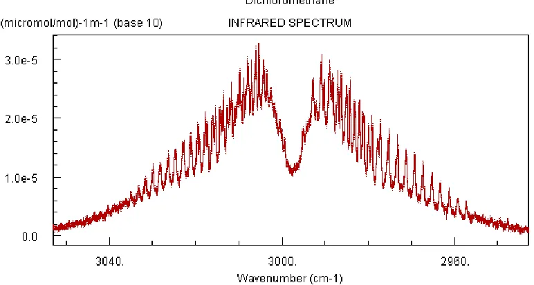
FIGURE 2.3 LWIR SPECTRUM OF DICHLOROMETHANE WITH P, Q, AND R BRANCHES, RES. 0.125 CM-1

Minor changes to the band shape will occur as the thermal energy available to the gas changes. A lower temperature will manifest itself as a contraction of the bands towards the central vibrational transition, with a slight bias towards the P branch. Conversely, heating the gas will promote the population to higher rotational levels, broadening the bands and lowering the intensity of each individual line as the population becomes spread thin.

Factors that affect the position of each successive rotational line include centrifugal distortion and the rotational inertia of the molecule. The effects of centrifugal distortion become increasingly important at high rotational energies. The faster the molecule spins, the greater affect “centrifugal force” will have in causing the internuclear separation to increase beyond that associated with the given vibrational energy for a given vibrational mode. When the internuclear separation increases, there is a resultant increase in the rotational inertia causing an overall decrease in spacing between adjacent rotational lines. Additionally, the reduced mass, which is a component of the rotational inertia, is essentially a ratio of the masses of the atoms in the molecule. The reduced mass influences the energy required to increase the rotation of a molecule and manifests itself as the primary driver of separation between rotational lines. The rotational sensitivity to mass is so great that if one had sufficient spectral resolution, the line positions between two isotopes of one atom in a molecule (with a reasonable contrast in mass) could be resolved, even though the mass difference is only that of one or two neutrons (1.675 x 10-24 g/neutron). This phenomenon manifests itself as rotational peak “doublets”, or pairs, with intensities that correspond to the abundance of the isotopic species in the sample.

(26)

11

[image:26.612.107.493.196.402.2]

few bands representing a few different vibrational modes are generally sufficient to identify a gas. Furthermore, little can be obtained about the rotational, or vibrational, temperature of the gas from the band shape at this resolution as the data are only suited to the coarsest of estimates. The figure below illustrates many of the points from this section including the distinctness of the P and R branches, the appearance of rotational lines in a ro-vibrational band that are partially discernable, and isotopic splitting of rotational lines from the two isotopes of chlorine.

FIGURE 2.4 INFRARED SPECTRUM OF DICHLOROMETHANE, RES. 0.125 CM-1

Note that both of the figures from this section showing the spectrum of dichloromethane illustrate the point made where the particular mode of vibration either allows for, or prevents the Q branch transitions from occurring. Figure 2.4 indicates a stretching mode, while Figure 2.3 represents a type of bend known as a deformation, which changes the molecular symmetry allowing for a change in orbital angular momentum.

2.2 Solid Phase Spectroscopy

While the purpose of this work is to identify chemical species in the gas phase, a major portion of the observed spectrum will be due to solid phase spectral phenomena. This portion of a spectrum generally comprises the background (minus atmosphere) of whatever the down-looking sensor “sees” behind/through the target gas.

(27)

12

(Patterson & Bailey, 2007). All of these factors combine to essentially smear out what was once the discrete spectral nature of entities in the gas phase. In fact, the emission spectrum of a solid is generally well modeled by a continuous function known as the Planck Black Body Equation, equation 2.1, with units of spectral radiance

(2.1)

where the constants and parameters include Planck’s constant (h) [J s], the speed of light (c) [m/s], Boltzmann’s constant (k) [J/K], the temperature of the radiator (T) [K], and the given wavelength of emission (λ) [micron]. It is clear that the equation is dependent on the Boltzmann population of the system at a given temperature. This allows one to model the limits of the energy available to each transition of a given wavelength, resulting in the characteristic short wavelength-side drop-off associated with black body radiation.

The construct of a black body is such that an optically opaque, reflectionless physical environment exists in which an emitted photon is absorbed and re-emitted multiple times before it exits the system. As such, the black body model is well suited to describe solids, but also models the general emission from liquids and even extremely dense gases such as the sun.

While the task of background removal would be straightforward if all one needed were the temperature and a Planck black body model, real backgrounds are not so cooperative. Virtually all background materials need to be modulated by a term known as emissivity to bring the predicted black body radiance in line with observed measurements. When energy in the form of a photon impinges on a solid, there are multiple possibilities as to what may happen. Depending on the material properties of the solid, the energy may be redirected in the form of reflection, transmitted through the solid, or absorbed by the solid. Conservation of energy suggests that the sum of the amount of energy reflected, transmitted, and absorbed should equal the total amount of energy incident on the solid. Further, Kirchoff’s law states that when it comes to emission, assuming the solid is in thermal equilibrium, a true black body will re-emit whatever is absorbed. This factor, which relates an amount of expected emission from the absorption, is known as emissivity. As can be seen from this example, even if one assumes a dense, optically opaque solid, some amount of energy will be lost to reflection, lowering the amount that can be absorbed, and thus directly lowering the emissivity. So to model a real solid, one must modulate the Planck predicted radiance by the emissivity, a value ranging from zero to one, resulting in what is known as a gray body.

(28)

13

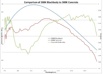
[image:28.612.85.514.193.501.2]

frequencies associated with optical phonons – the vibrational harmonics of the solid lattice, are in resonance and causes intense absorption. Restrahlen features, much like the ro-vibrational bands of gases, are often telltale indicators of the identity of component elements in a solid (Elachi & van Zyl, 2006). Figure 2.5 demonstrates the deviation from the Planck predicted radiance in the LWIR for concrete at 300K. The smooth curve in the chart is the Planck predicted blackbody radiance while the red trace immediately beneath it is the same 300K blackbody curve modulated by the emissivity spectrum of concrete, which is shown as the green trace that corresponds to the right vertical axis.

FIGURE 2.5 300K BLACKBODY COMPARISON TO 300K CONCRETE WITH EMISSIVITY OVERLAY

Clearly, background removal or modeling, which is a seemingly straightforward task, can now be seen to be exceedingly difficult depending on the composition of the solid. Fortunately, the discrete spectral features associated with the target gas one may be trying to identify in the collected spectrum are generally finer than those of the solids in the background. Thus, the gas-associated spectral features may appear to “ride on top” of the more slowly spectrally varying background features, still allowing for isolation or identification.

2.3 Atmospheric Effects in the LWIR

(29)

14

being homonuclear diatomics, possess no rhythmically transient net dipole and therefore, will be IR-inactive. Assuming for the moment that this premise is true, we will focus on the other one percent of the atmosphere that will have substantial influence on the LWIR remote sensing problem.

The following table, taken from the Handbook of Chemistry and Physics, illustrates a typical composition of the atmosphere at sea level.

TABLE 2.1 ATMOSPHERIC COMPOSITION AT SEA LEVEL (CHEMICAL RUBBER COMPANY, 1992)

Note that the noble gas argon is shown as taking up nearly the entire bulk of the remaining one percent of atmospheric constituents, yet argon has no vibrational or rotational modes and is only subject to electronic transitions. Thus, argon is not of concern for the purposes of this work. This leaves an exceedingly small amount of gases left that are responsible for the overwhelming atmospheric absorption features found throughout the infrared portion of the electromagnetic spectrum.

It is a combination of three gases that are responsible for the bulk of these atmospheric absorption features, particularly in the LWIR, yet some were not included in the table above. One of these gases that was notably left off of the composition table shown above is water. Water is extremely variable throughout the atmosphere and is highly dependent on geographic location and time of day, so it was not appropriate to include it in the list above. An additional gas left off of the table is ozone. This makes sense in that ozone is primarily a stratospheric gas and is generally found in negligible concentrations near the surface, outside of dense urban areas. Ozone concentrations are highly correlated to altitude and this impact to airborne remote sensing will be explored shortly. Finally, carbon dioxide, as shown in the table, is the prominent IR-active “mainstay” gas throughout the atmosphere and a primary atmospheric absorption culprit.

(30)

15

work, a subset of the LWIR window from approximately 8-12.5 microns (800-1250 cm-1) will be used. This window is flanked by absorptions from the bending mode of water near 8 microns, accompanied by the deformation mode of methane and stretching harmonic overtone of N2O. At

approximately 9.8 microns, ozone punches a hole in the window with a strong dual stretching mode, P and R branch band absorption feature. Finally, the bending mode of carbon dioxide fills in the long wavelength side of the window with an intense absorption. The LWIR window coincidently covers the spectral range where a majority of the gases of interest to remote sensing have significant ro-vibrational features, many of which occur coincidentally with ozone. These gases will be reviewed in detail in the next chapter.

Radiative transport in this work was accomplished via an atmospheric model called MODTRAN. MODTRAN (Moderate Resolution Atmospheric Transmission) was developed by the Air Force Geophysical Laboratory at Hanscom Air Force Base twenty years ago as an order of magnitude resolution improvement to the then current LOWTRAN 7 code (Low Resolution Atmospheric Transmission) (Berk, Bernstein, & Robertson, MODTRAN: A Moderate Resolution Model for LOWTRAN 7, 1989). MODTRAN generates transmission values by employing pre-determined column densities of various component atmospheric gases, such as the 1976 US standard atmosphere, and sums their absorption across the spectral bands of interest. These terms are then applied to the path the radiance is to travel in both height and angle through the atmosphere. Finally, scattering is considered based on visibility/aerosol loading and environment selected (urban/rural) accounting for radiance scattered in and out of the signal path through multiple scattering events. These absorption and scattering events are built into layers that keep track of the radiance attenuation through the entire path length. Finally, radiance produced by the sun based on time of day and date is considered as well as adverse weather conditions the user may select such as rain, ice, clouds, or differing amounts of component gases and aerosols. These radiance values are then assembled, sampled by the instrument resolution provided, and output into large tables detailing the individual contributions of the various effects. The careful consideration and improvements that have gone into the construction of MODTRAN over the last several decades of its existence have made it the industry standard in moderate resolution atmospheric modeling for remote sensing use.

(31)

[image:31.612.89.506.98.369.2]

16

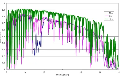
FIGURE 2.6 ATMOSPHERIC ABSORPTION PROFILE BY ALTITUDE IN THE LWIR

Several important points can be made from Figure 2.6. Clearly, individual rotational lines, primarily due to water, can be seen throughout the spectrum. This range of rotational lines, which extends well through the far infrared to the microwave is known as the water rotational continuum (Wozniak & Dera, 2007). Rotational lines for water have a large rotational constant (energy spacing) due to the decreased reduced mass and therefore, decreased rotational inertia, thus it is not unreasonable to be able to resolve individual rotational lines of water. Conversely, carbon dioxide and ozone have comparatively smaller rotational constants due to a much larger rotational inertia resulting in closely spaced rotational lines that form the more recognizable band shapes seen in earlier example spectra.

(32)

17

shows that both Rayleigh (molecular) scattering, which is most prominent among shorter wavelengths in the visible, and aerosol scattering have minimal impact to the transmission in the LWIR. Should scattering have had a greater impact, a slope of reduced transmission proportional to λ-4 would have been more evident.

As many gases have prominent features in the 9-10 micron region of the LWIR, and due to the significant sensitivity and variability of ozone absorption with altitude, it seems prudent to restrict the operational altitude of a given aerial collection vehicle to approximately one, and at most, five kilometers for the purposes of this study.

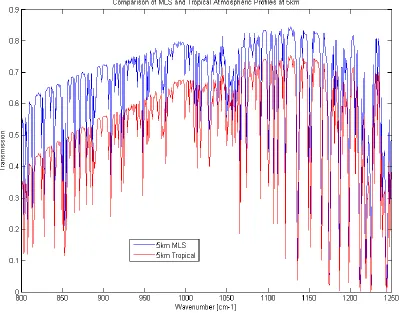
[image:32.612.99.498.322.636.2]

As previously demonstrated, the majority of absorption due to water vapor in the atmosphere will occur in the first 5 kilometers of altitude however, the extent of that absorption is dependent on current humidity conditions. Figure 2.7 shows an example of a mid-latitude summer (MLS) standard atmosphere model from MODTRAN compared to a tropical model at 5 km altitude. Note the increased absorption and overall reduced transmission due to nearly double the total column water vapor content. Both of these atmospheric models are employed in this work.

FIGURE 2.7 COMPARISON OF TROPICAL AND MLS ATMOSPHERIC MODELS AT 5KM

(33)

18

analysis of both the up and down-welled radiance that accompanies the target radiance, among other sources. This analysis can be accomplished via radiometric modeling.

2.4 Mathematically Modeling the Sensor Reaching Spectral Radiance of a

Gas

Developing a model to determine the sensor-reaching radiance for the gas detection problem is not a straightforward task and requires multiple assumptions. In the LWIR, the main drivers of signal in a collected spectrum will come from the target gas itself (assuming it is present in the scene), the background, and the atmosphere. Secondary effects from reflections and other sources of stray radiation can be shown to have minimal impact to the overall collected radiance for natural materials (Tonooka, 2001). The development of this sensor reaching radiance model illustrates the foundation of the radiative transport methods implemented in the FTS simulation code used in this work.

2.4.1 Model Assumptions and Mathematical Development

Beginning with the background, which can be modeled as a modified black body radiator as previously established, a temperature must be set to govern the strength of the emission. This temperature can be extracted from brightness or apparent temperature studies of the scene, through a priori knowledge of the conditions in the scene, or through an educated guess (Boonmee, 2007). For the sake of simplicity, the latter method will be used. Next, the emissivity at a given wavelength must be determined. Spectral emissivity estimation can involve methods that are quite complex, and again, for the purposes of simplicity, it can be shown that in the absence of a priori emissivity knowledge, a flat estimate of 0.9 across the LWIR spectral range is a reasonable assumption, particularly from nadir observations (Tonooka, 2001). For this work, actual spectral collects of materials such as concrete, asphalt, steel, and sand taken from Trona, California by members of the Digital Imaging and Remote Sensing (DIRS) group at the Center for Imaging Science (CIS) at the Rochester Institute of Technology (RIT) will be used as background sources. These collects were analyzed by the group to produce emissivity curves in the LWIR and can be imported directly to any model requiring no emissivity or temperature estimates. Finally, in a direct line-of-sight (LOS) to the sensor, the only other impact to the background radiance is the contribution from the atmosphere on a per wavelength basis, which is aptly modeled by the MODTRAN software.

(34)

19

[image:34.612.100.488.126.442.2]

up and down-welled radiance derived from MODTRAN using a 1 km tropical atmosphere and a 0.9 constant emissivity gray body surface.

FIGURE 2.8 MODELED UP AND DOWN-WELLED RADIANCE

(35)

20

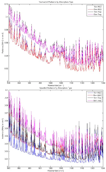
[image:35.612.125.469.111.670.2]

panels show the differences and similarities between the up and down-welled radiance profiles for each atmospheric model used in this work.

(36)

21

Figure 2.9 shows the spectral nature of each profile type. Both profiles are in emission as they are generated by the self-emission of the atmosphere. The downwelled radiance shown in the top panel represents the entire atmosphere’s emission impinging on the surface. Note the substantial contribution from ozone. Also note however, that the strength of the emission is more dependent on atmospheric profile than altitude. This is because the altitude given is for the sensor height, whereas the downwelled comes from the contribution of the entire atmosphere. Therefore, the only influence to the total radiance comes from the amount of radiators in the atmosphere. With the tropical profile containing twice the water content of the MLS, there is a significant difference in the amount of radiating species. The upwelled radiance, which considers the self-emission of the atmosphere into the path of the collected radiance, is dependent on how much atmosphere is contained between the ground and sensor. As expected, the higher the altitude, or larger number of emitting species, the higher the contribution to the total radiance. Of interest is the proximity of the 5km MLS upwelled radiance profile to the 1km tropical profile. The additional 4km in altitude of the MLS profile is approximated by the increase in water vapor of the tropical profile.

To aid in the development of a sensor reaching radiance model, several assumptions can be made. For the moment, assume that if primarily natural surface materials are considered, the assumption of no reflected radiance serves to eliminate many second order terms including down-welled radiance, that when taken in bulk, have minimal overall effect. However, up-welled radiance, generated in the atmosphere along the sensor line-of-sight, becomes an important consideration and will contribute to the total sensor-reaching radiance. This quantity varies with wavelength at a given altitude across the LWIR window chosen for this work and can be modeled as a wavelength dependent additive term. To this point the sensor reaching radiance is modeled by equation 2.2,

(2.2)

where λ is the wavelength of interest, T is the temperature of the background, B, which is modulated by a wavelength dependent emissivity term, ε, and the atmospheric transmission, τ, and the last term represents the up-welled radiance with units: [W m-2 sr-1 µm-1]. The magnitude of both the atmospheric transmission and up-welled radiance is of course dependent on the altitude for which the model is implemented. To this point the model simply illustrates the sensor reaching radiance due to the self-emission of a surface material through the atmosphere with an additive up-welled radiance.

(37)

22

selective radiator. Essentially, if one can link the value of the emissivity via the absorptivity of the gas, the black body model will provide the estimate of thermally available energy at each line position, which is then modulated via the absorptivity of the gas. It turns out that establishing the link from emissivity to absorptivity is rather straightforward.

First, we start with Beer’s law, which states that the absorbance at a given wavelength is directly proportional to the absorptivity of the given species, the path length of the measurement through the species, and the concentration of the species. This relationship is shown in equation 2.3

(2.3)

where absorbance is on a per wavelength basis and is unitless, kappa is the absorptivity on a per wavelength basis with units of reciprocal concentration and reciprocal distance [ppm-1 m-1] , l [m] is the path length in units of distance, and c is concentration [ppm], often in units of parts per million. While epsilon is historically used to represent absorptivity, kappa has been substituted to prevent confusion with the symbol for emissivity. Figure 2.12 shows an example of an absorptivity spectrum of a gas in the LWIR.

Recalling the conservation of energy for photon interaction with a solid mentioned in section 2.2, if we assume that the gas is optically thin and has essentially no reflection, the only terms left are transmission and absorption. Starting from this assumption, we next assume that the system is in LTE and can then say that Kirchhoff’s law of emissivity being equal to absorbance applies. Then, it can be shown that the transmission through the gas is one minus the emissivity, which is equal to the expression for absorbance shown above. This development is shown in equation 2.4 as

(2.4)

where the last step shows the equation has been solved for transmission. These equations allow for a direct replacement of the emissivity term with the absorptivity and concentration-path length value for the modulation of the gas emission. The transmission equation allows the background to be modulated by the absorptivity of the gas as it passes through the plume as prescribed by Beer’s law. Beer’s law has been shown to remain a linear relationship for low concentrations up to 250,000 ppm (Skoog, Holler, & Nieman, 1998).

(38)

23

(2.5)

where the new S and P subscripts indicate a parameter belonging to the surface or the gas plume, respectively. The subscript a attributes the transmission attenuation to the atmosphere. Note that the background radiance is attenuated by the transmission through the gas plume, whereas the sum of both the background and plume radiance is attenuated by the atmosphere. One may ask where the term is that represents the up-welled radiance generated from the atmosphere below the plume and is attenuated by the plume as it travels toward the sensor. This term may be neglected if it is assumed that the plume is sufficiently low to the ground that the space between it and the surface is negligible, resulting in minimal up-welled radiance. All gas plumes in this work are considered to be gas leaks and will therefore be essentially at ground level, supporting the assumption. This equation represented the SRR model for the early portion of this work, where surface materials only had up to a maximum of 15% reflectivity and resulted in minimal contributions from down-welled radiance.

Due to the fact that not all surface materials encountered in the real world will be near perfect black bodies, removing the assumption of neglecting the down-welled radiance is in order and results in the following modification to equation 2.5

(2.6)

where the new radiance term, Ld, is the down-welled radiance, modulated by the surface

reflectance and the gas plume, then transported to the sensor via the atmospheric transmission. This equation represents the radiative transport model used in this work for a single gas, atmosphere, and surface material and as handled by the DIRSIG SRR model covered in section 3.1.7.

2.4.2 Characterizing Model Behavior

A close analysis of equation 2.6 shows that in spectral regions where the absorptivity is near zero, the gas term becomes negligible and the background term dominates. Conversely, when the plume is maximally absorbing, the transmission of the background radiance drops to zero. Aside from the concentration-path length product term, which dictates the “strength” of the given absorption, the temperature difference between the background and plume is a major driver in the “visibility” of the plume spectrum over the background. If the plume contains sufficient thermal energy, it will appear in emission and essentially ride on top of whatever the background radiance may be beneath it. If the plume lacks thermal energy, it will appear as an absorption feature due to the selective absorption of energy from the background radiance as it passes through the plume. This behavior is essentially identical to transmission of the background through another layer of atmosphere – albeit of differing composition. One can now see that in order to detect the presence of the plume in the observed spectrum, there needs to be sufficient thermal contrast between the plume and background.

Figure 2.10 demonstrates the concept of thermal contrast and was generated using both 290K and 310K CH3Cl at 11,500 ppm-m with no atmosphere, over a flat 0.9 emissivity black body background

(39)

24

the same, the magnitude of the radiance values for a given absorption feature in emission compared to absorption are not. This is a result of the emissivity value being less than one. As can be seen from equation 2.6, at an emissivity of one and with a thermal contrast of zero, no spectral features should be visible, as expected. However, if the emissivity is reduced, even when the thermal contrast is still zero, the gas will appear in emission. In fact, depending on how low the emissivity becomes, the thermal contrast can be negative indicating absorption, while the spectrum will still be in emission. Said another way, there must be a difference in brightness temperature between the gas and surface for the plume to be visible in the recorded spectrum.

FIGURE 2.10 THERMAL CONTRAST COMPARISON FOR CH3Cl IN ABSORPTION (LEFT) AND EMISSION (RIGHT)

(40)

[image:40.612.106.482.84.383.2]

25

FIGURE 2.11 AMMONIA/ASPHALT IN BOTH EMISSION AND ABSORPTION (TOP) AND ASPHALT EMISSIVITY (BOTTOM)

Clearly, any attempt at species identification, or even detection, via a quantitative spectral scoring metric will require accuracy in both the absorption and emission regimes.

2.4.3 PNNL Gas Absorptivity Library

Absorptivity values for all gases used in this work were derived from the Pacific Northwest National Labs (PNNL) Quantitative IR database for Infrared Remote Sensing and Hyperspectral Imaging. The PNNL spectral gas database is a compilation of over 500 gas-phase spectra collected in pressurized vessels to simulate the anticipated atmospheric broadening one would observe under typical remote sensing conditions (Sharpe, Sams, & Johnson, 2002). The data are collected with high resolution (0.10 cm-1, 1 nm at 10 µm) FTS systems at three different temperatures: 278, 298, and 323K. The approach of this work is to use the 298K data and change the black body temperature of the gas model within a bracketed range of this value. While further extrapolation of the absorptivity values between those provided by PNNL at the three baseline temperatures may result in slightly more accurate values, making an assumption as to the behavior of the absorptivity over these temperature ranges (i.e., linear) may introduce more error than benefit.

(41)

26

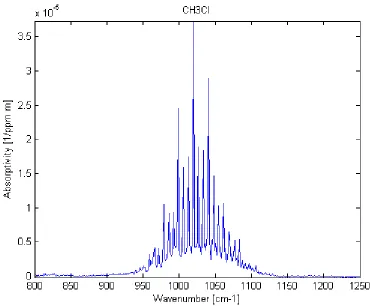
[image:41.612.108.478.116.422.2]

reported in values of absorptivity, making applications to modeling efforts seamless. Figure 2.12 is an example of the PNNL output for an absorption feature of CH3Cl gas at 298K in the LWIR.

FIGURE 2.12 PNNL DATABASE ABSORPTIVITY SPECTRUM FOR CH3Cl GAS IN THE LWIR

2.5 Fourier Transform Infrared Spectrometers

(42)

27

phase shift so that the only phase difference between the two beams upon recombination is due to the difference in optical path traveled.

FIGURE 2.13 MICHELSON INTERFEROMETER AS A SPECTROMETER (BEER, 1992)

2.5.1 FTS Advantages

FTS are known to have several advantages over dispersive element spectrometers (DES) (Carter, Bennett, Fields, & Hernandez, 1993). One such advantage is called the Jacquinot advantage. The Jacquinot advantage describes the system etendue, which is a measure of the product of the maximum beam area and solid angle of the beam passing through the system. In spectrometers, the limiting optical element is typically the most expensive element to manufacture in a large size. For dispersive systems, this would be the grating and for FTS, the beam splitter. For comparably sized instruments, an FTS can be shown to have a system entendue over 150x greater than that of a dispersive system (Beer, 1992). While it is true that a much larger grating can be made to compensate for the system entendue as compared to a similar sized beam splitter, the FTS can maintain a substantially smaller and more compact instrument footprint while maintaining a similar entendue.

The Fellgett advantage describes the frequency-division multiplexing advantage of an FTS as compared to a DES. Initially, this advantage was made in comparison of the detection schemes of FTS and DES in which scanning a dispersive element across a single photodiode to collect an entire spectrum was compared to the simultaneous observation of all transmittable frequencies in a given spectrum in an FTS. With the advent of arrayed detectors, a DES can now collect multiple ‘bands’ across a given spectrum simultaneously. The problem here is that the size of the resulting spectral coverage is dependent on the amount of dispersion associated with the element, which ultimately becomes limited by the sensitivity of the detector for a given source intensity.