Heavy-tailed distributions : data, diagnostics, and new developments

(1)

1616 P St. NW

Washington, DC 20036 202-328-5000 www.rff.org

MM March 2011 _{RFF DP 11-19}

Heavy-Tailed

Distributions: Data,

Diagnostics, and New

Developments

Roger M. Cooke and Daan Nieboer

(2)

Resources for the Future

Department of Mathematics, Delft University of Technology

Heavy-Tailed Distributions:

Data, Diagnostics and New Developments

Roger M. Cooke and Daan Nieboer

March 2011

(3)

Abstract

This monograph is written for the numerate nonspecialist, and hopes to serve three purposes. First it gathers mathematical material from diverse but related ﬁelds of order statistics, records, extreme value theory, majorization, regular variation and subexponentiality. All of these are relevant for understanding fat tails, but they are not, to our knowledge, brought together in a single source for the target readership. Proofs that give insight are included, but for fussy calculations the reader is referred to the excellent sources referenced in the text. Multivariate extremes are not treated. This allows us to present material spread over hundreds of pages in specialist texts in twenty pages. Chapter 5 develops new material on heavy tail diagnostics and gives more mathematical detail.

Second, it presents a new measure of obesity. The most popular definitions in terms of regular variation and subexponentiality invoke putative properties that hold at infinity, and this complicates any empirical estimate. Each definition captures some but not all of the intuitions associated with tail heaviness. Chapter 5 studies two candidate indices of tail heaviness based on the tendency of the mean excess plot to collapse as data are aggregated. The probability that the largest value is more than twice the second largest has intuitive appeal but its estimator has

very poor accuracy. The Obesity indexis deﬁned for a positive random variable X as:

Ob(X) =P(X1+X4 > X2+X3|X1≤X2 ≤X3≤X4), Xiindependent copies of X.

For empirical distributions, obesity is deﬁned by bootstrapping. This index reasonably captures

intuitions of tail heaviness. Among its properties, if α > 1 then Ob(X) < Ob(Xα). However,

it does not completely mimic the tail index of regularly varying distributions, or the extreme

value index. A Weibull distribution with shape 1/4 is more obese than a Pareto distribution

with tail index 1, even though this Pareto has inﬁnite mean and the Weibull’s moments are all ﬁnite. Chapter 5 explores properties of the Obesity index.

Third and most important, we hope to convince the reader that fat tail phenomena pose real problems; they are really out there and they seriously challenge our usual ways of thinking about historical averages, outliers, trends, regression coefficients and confidence bounds among many other things. Data on flood insurance claims, crop loss claims, hospital discharge bills, precipitation and damages and fatalities from natural catastrophes drive this point home.

(4)

Chapter 1 Fatness of Tail

1.1 Fat tail heuristics

Suppose the tallest person you have ever seen was 2 meters (6 feet 8 inches); someday you may meet a taller person, how tall do you think that person will be, 2.1 meters (7 feet)? What is the probability that the ﬁrst person you meet taller than 2 meters will be more than twice as tall, 13 feet 4 inches? Surely that probability is inﬁnitesimal. The tallest person in the world, Bao Xishun of Inner Mongolia,China is 2.36 m or 7 ft 9 in. Prior to 2005 the most costly Hurricane in the US was Hurricane Andrew (1992) at $41.5 billion USD(2011). Hurricane Katrina was

the next record hurricane, weighing in at $91 billion USD(2011)1. People’s height is a ”thin

tailed” distribution, whereas hurricane damage is ”fat tailed” or ”heavy tailed”. The ways in which we reason from historical data and the ways we think about the future are - or should be - very diﬀerent depending on whether we are dealing with thin or fat tailed phenomena. This monograph gives an intuitive introduction to fat tailed phenomena, followed by a rigorous

mathematical treatment of many of these intuitive features. A major goal is to provide a

deﬁnition of Obesity that applies equally to ﬁnite data sets and to parametric distribution

functions.

Fat tails have entered popular discourse largely thanks to Nassim Taleb’s book The Black

Swan, the impact of the highly improbable (Taleb [2007]). The black swan is the paradigm shat-tering, game changing incursion from ”extremistan” which confounds the unsuspecting public, the experts, and especially the professional statisticians, all of whom inhabit ”mediocristan”.

Mathematicians have used at least three main deﬁnitions of tail obesity. Older texts some-time speak of ”leptokurtic distributions”, that is, distributions whose extreme values are ”more

probable than normal”. These are distributions with kurtosis greater than zero2, and whose

tails go to zero slower than the normal distribution.

Another deﬁnition is based on the theory of regularly varying functions and characterizes

the rate at which the probability of values greater than x goes to zero as x → ∞. For a

large class of distributions this rate is polynomial. Unless otherwise indicated, we will always

consider non-negative random variables. LettingF denote the distribution function of random

variable X, such that S(x) = 1−F(x) = P rob{X > x}, we write S(x) ∼ x−α, x → ∞ to

mean S_x(−xα) → 1, x → ∞. S(x) is called the survivor function of X. A survivor function with

polynomial decay rate−α, or as we shall saytail index α, has inﬁniteκthmoments for allκ≥α.

If we are ”suﬃciently close” to inﬁnity to estimate the tail indices of two distributions, then we can meaningfully compare their tail heaviness by comparing their tail indices, and many

1

http://en.wikipedia.org/wiki/Hurricane Katrina, accessed January 28, 2011 2

Kurtosis is defined as the (µ4/σ4)−3 whereµ4is the fourth central moment, andσis the standard deviation. Subtracting 3 arranges that the kurtosis of the normal distribution is zero

(7)

intuitive features of fat tailed phenomena fall neatly into place. The Pareto distribution is a special case of a regularly varying distribution where S(x) =x−α, x >1.

A third deﬁnition is based on the idea that the sum of independent copies X1+X2+, . . . Xn

behaves like the maximum ofX1, X2, . . . Xn. Distributions satisfying

P rob{X1+X2+,· · ·+Xn> x} ∼P rob{M ax{X1, X2, . . . Xn}> x}, x→ ∞

are calledsubexponential. Like regular variation, subexponality is a phenomenon that is deﬁned

in terms of limiting behavior as the underlying variable goes to inﬁnity. Unlike regular variation, there is no such thing as an ”index of subexponality” that would tell us whether one distribution is ”more subexponential” than another. The set of regularly varying distributions is a strict subclass of the set of subexponential distributions. Other more exotic deﬁnitions are given in chapter 4.

There is a swarm of intuitive notions regarding heavy tailed phenomena that are captured to varying degree in the diﬀerent formal deﬁnitions. The main intuitions are:

• The historical averages are unreliable for prediction

• Diﬀerences between successively larger observations increases

• The ratio of successive record values does not decrease;

• The expected excess above a threshold, given that the threshold is exceeded, increases as

the threshold increases

• The uncertainty in the average of nindependent variables does not converge to a normal

with vanishing spread as n→ ∞; rather, the average is similar to the original variables.

1.2 History and Data

A colorful history of fat tailed distributions is found in (Mandelbrot and Hudson [2008]). Man-delbrot himself introduced fat tails into finance by showing that the change in cotton prices was heavy-tailed (Mandelbrot [1963]). Since then many other examples of heavy-tailed distri-butions are found, among these are data file traffic on the internet (Crovella and Bestavros [1997]), returns on financial markets (Rachev [2003], Embrechts et al. [1997]) and magnitudes of earthquakes and floods (Latchman et al. [2008], Malamud and Turcotte [2006]).

Data for this monograph were developed in the NSF project 0960865, and are available from http : //www.rf f.org/Events/P ages/Introduction−Climate−Change−Extreme− Events.aspx, or at public cites indicated below.

1.2.1 US Flood Insurance Claims

US flood insurance claims data from the National Flood Insurance Program (NFIP) are aggre-gated by county and year for the years 1980 to 2008. The data are in 2000 US dollars. Over this time period there has been substantial growth in exosure to flood risk, particularly in coastal counties. To remove the effect of growing exposure, the claims are divided by personal income estimates per county per year from the Bureau of Economic Accounts (BEA). Thus, we study

ﬂood claims per dollar income, by county and year3.

(8)

1.3. DIAGNOSTICS FOR HEAVY TAILED PHENOMENA 7

1.2.2 US Crop Loss

US crop insurance indemnities paid from the US Department of Agriculture’s Risk Management Agency are aggregated by county and year for the years 1980 to 2008. The data are in 2000 US dollars. The crop loss claims are not exposure adjusted, as a proxy for exposure is not obvious,

and exposure growth is less of a concern.4

1.2.3 US Damages and Fatalities from Natural Disasters

The SHELDUS database, maintained by the Hazards and Vulnerability Research Group at the University of South Carolina, has county-level damages and fatalities from weather events. Infor-mation on SHELDUS is available online: http://webra.cas.sc.edu/hvri/products/SHELDUS.aspx. The damage and fatality estimates in SHELDUS are minimum estimates as the approach to com-piling the data always takes the most conservative estimates. Moreover, when a disaster aﬀected many counties, the total damages and fatalities were apportioned equally over the aﬀected coun-ties, regardless of population or infrastructure. These data should therefore be seen as indicative rather than as precise.

1.2.4 US Hospital Discharge Bills

Billing data for hospital discharges for a northeastern US state were collected over the years 2000 - 2008. The data is in 2000 USD.

1.2.5 G-Econ data

This uses the G-Econ database (Nordhaus et al. [2006]) showing the dependence of Gross Cell Product (GCP) on geographic variables measured on a spatial scale of one degree. At 45 latitude, a one by one degree grid cell is [45mi]2_{or [68}_km_]2_{. The size varies substantially from equator to} pole. The population per grid cell varies from 0.31411 to 26,443,000. The Gross Cell Product is for 1990, non-mineral, 1995 USD, converted at market exchange rates. It varies from 0.000103

to 1,155,800 USD(1995), the units are $106_{. The GCP per person varies from 0.00000354 to}

0.905, which scales from $3.54 to $905,000. There are 27,445 grid cells. Throwing out zero and empty cells for population and GCP leaves 17,722; excluding cells with empty temperature data leaves 17,015 cells.

The data are publicly available at http://gecon.yale.edu/world big.html.

1.3 Diagnostics for Heavy Tailed Phenomena

Once we start looking, we can ﬁnd heavy tailed phenomena all around us. Loss distributions are a very good place to look for tail obesity, but something as mundane as hospital discharge billing data can also produce surprising evidence. Many of the features of heavy tailed phenomena would render our traditional statistical tools useless at best, dangerous at worst. Prognosticators base

predictions on historical averages. Of course, on a ﬁnite sample the average and standard

deviation are always ﬁnite; but these may not be converging to anything and their value for prediction might be nihil. Or again, if we feed a data set into a statistical regression package, the regression coeﬃcients will be estimated as ”covariance over the variance”. The sample versions of these quantities always exist, but if they aren’t converging, their ratio could whiplash wildly, taking our predictions with them. In this section, simple diagnostic tools for detecting tail obesity are illustrated on mathematical distributions and on real data.

(9)

1.3.1 Historical Averages

Consider independent and identically distributed random variables with tail index 1 < α < 2.

The variance of these random variables is inﬁnite, as is the variance of any ﬁnite sum of these

variables. In consequence, the variance of the average of n variables is also inﬁnite, for any

n. The mean value is ﬁnite and is equal to the expected value of the historical average, but

regardless how many samples we take, the average does not converge to the variable’s mean,

and we cannot use the sample average to estimate the mean reliably. Ifα <1 the variables have

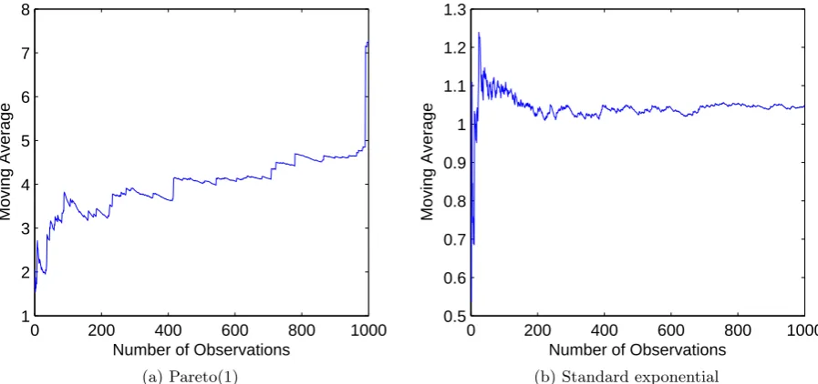
infinite mean. Of course the average of any finite sample is finite, but as we draw more samples, this sample average tends to increase. One might mistakenly conclude that there is a time trend in such data. The universe is finite and an empirical sample would exhaust all data before it reached infinity. However, such re-assurance is quite illusory; the question is, ”where is the sample average going?”. A simple computer experiment suffices to convince the sceptic: sample a set of random numbers on your computer, these are approximately independent realizations of a uniform variable on the interval [0,1]. Now invert these numbers. If U is such a uniform variable, 1/U is a Pareto variable with tail index 1. Compute the moving averages and see how well you can predict the next value.

Figure 1.1 (a)–(b) shows the moving average of respectively a Pareto(1) distribution and a standard exponential distribution. The mean of the Pareto(1) distribution is inﬁnite whilst the mean of the standard exponential distributions is equal to one.

0 200 400 600 800 1000

1 2 3 4 5 6 7 8

Number of Observations

Moving Average

(a) Pareto(1)

0 200 400 600 800 1000

0.5 0.6 0.7 0.8 0.9 1 1.1 1.2 1.3

Number of Observations

Moving Average

[image:9.595.72.521.385.596.2]

(b) Standard exponential

Figure 1.1: Moving average of Pareto(1) and standard exponential data

As we can see, the moving average of the Pareto(1) distribution shows an upward trend, whilst the moving average of the Standard Exponential distribution converges to the real mean

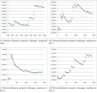
of the Standard Exponential distribution. Figure 1.2 (a) shows the moving average of US

(10)

(a) Natural disaster property damage, temporal order

(b) Natural disaster property damage, random or-der 1

(c) Natural disaster property damage, random or-der 2

(d) Natural disaster property damage, random or-der 3

Figure 1.2: Moving average US natural disaster property damage

1.3.2 Records

One characteristic of heavy-tailed distributions is that there are usually a few very large values compared to the other values of the data set. In the insurance business this is called the Pareto law or the 20-80 rule-of-thumb: 20% of the claims account for 80% of the total claim amount in an insurance portfolio. This suggests that the largest values in a heavy tailed data set tend to be further apart than smaller values. For regularly varying distributions the ratio between the two largest values in a data set has a non-degenerate limiting distribution, whereas for distributions like the normal and exponential distribution this ratio tends to zero as we increase the number of observations. If we order a data set from a Pareto distribution, then the ratio between two consecutive observations also has a Pareto distribution. In Table 1.1 we see the

Number of observations standard normal distribution Pareto(1) distribution

10 0.2343 1₂

50 0.0102 1₂

[image:10.595.113.514.88.472.2]

100 0.0020 1₂

(11)

probability that the largest value in the data set is twice as large as the second largest value for the standard normal distribution and the Pareto(1) distribution. The probability stays constant for the Pareto distribution, but it tends to zero for the standard normal distribution as the number of observations increases.

[image:11.595.66.501.210.429.2]

Seeing that one or two very large data points confound their models, unwary actuaries may declare these ”outliers” and discard them, re-assured that the remaining data look ”normal”. Figure 1.3 shows the yearly diﬀerence between insurance premiums and claims of the U.S. National Flood Insurance Program (NFIP) (Cooke and Kousky [2009]).

Figure 1.3: US National Flood Insurance Program, premiums minus claims

The actuaries who set NFIP insurance rates explain that their ”historical average” gives 1% weight to the 2005 results including losses from hurricanes Katrina, Rita, and Wilma: ”This is an attempt to reﬂect the events of 2005 without allowing them to overwhelm the pre-Katrina experience of the Program” (Hayes and Neal [2011] p.6)

1.3.3 Mean Excess

The mean excess function of a random variable X is deﬁned as:

e(u) =E[X−u|X > u] (1.1)

The mean excess function gives the expected excess of a random variable over a certain threshold given that this random variable is larger than the threshold. It is shown in chapter 4 that

subexponential distributions’ mean excess function tends to inﬁnity as u tends to inﬁnity. If

we know that an observation from a subexponential distribution is above a very high threshold then we expect that this observation is much larger than the threshold. More intuitively, we should expect the next worst case to be much worse than the current worst case. It is also shown

that regularly varying distributions with tail indexα >1, have a mean excess function which is

ultimately linear with slope _α₋1₁. If α <1, then the slope is inﬁnite and (1.1) is not useful. If

we order a sample of n independent realizations of X, we can construct a mean excess plot as

(12)

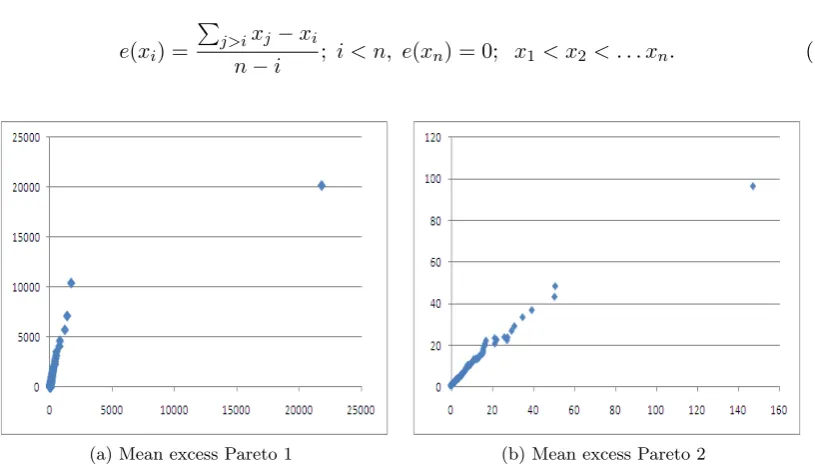
e(xi) =

∑

j>ixj−xi

n−i ; i < n, e(xn) = 0; x1 < x2 < . . . xn. (1.2)

[image:12.595.113.521.91.327.2]

(a) Mean excess Pareto 1 (b) Mean excess Pareto 2

Figure 1.4: Pareto mean excess plots, 5000 samples

Figure 1.4 shows mean excess plots of 5000 samples from a Pareto(1) (a) and a Pareto(2) (b). Clearly, eyeballing the slope in these plots gives a better diagnostic for (b) than for (a).

(a) Mean excess flood claims/income (b) Mean excess crop loss

Figure 1.5: Mean excess plots, ﬂood and crop loss

Figure 1.5 shows mean excess plots for ﬂood claims per county per year per dollar income (a), and insurance claims for crop loss per year per county (b). Both plots are based on roughly the top 5000 entries.

1.3.4 Sum convergence: Self-similar or Normal

For regularly varying random variables with tail indexα <2 the standard central limit theorem

(13)

This can be observed in the mean excess plot of data sets of 5000 samples from a regularly varying distribution. In the mean excess plot the empirical mean excess function of a data set

is plotted. Deﬁne the operationaggregating by kas dividing a data set randomly into groups of

sizek and summing each of thesekvalues. If we consider a data set of size nand compare the

mean excess plot of this data set with the mean excess plot of a data set we obtained through

aggregating the original data set byk, then we ﬁnd that both mean excess plots are very similar.

Whereas for data sets from thin-tailed distributions both mean excess plots look very diﬀerent.

0.0 0.2 0.4 0.6 0.8 1.0

0.0

0.2

0.4

0.6

0.8

1.0

Threshold

Mean Excess

Original Dataset Aggregation by 10 Aggregation by 50

(a) Exponential distribution

0.0 0.2 0.4 0.6 0.8 1.0

0.0

0.2

0.4

0.6

0.8

1.0

Threshold

Mean Excess

(b) Paretoα= 1

0.2 0.4 0.6 0.8 1.0

0.0

0.2

0.4

0.6

0.8

1.0

Threshold

Mean Excess

(c) Paretoα= 2

0.0 0.2 0.4 0.6 0.8 1.0

0.0

0.2

0.4

0.6

0.8

1.0

Threshold

Mean Excess

[image:13.595.60.487.246.697.2]

(d) Weibull distributionτ= 0.5

Figure 1.6: Standardized mean excess plots

(14)

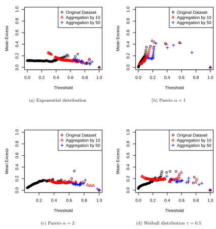
excess plot, since we can easily see that e(cu) = ce(u). Figure 1.6 (a)–(d) shows the

standard-ized mean excess plot of a sample from an exponential distribution, a Pareto(1) distribution, a Pareto(2) distribution and a Weibull distribution with shape parameter 0.5. Also shown in each plot are the standardized mean excess plots of a data set obtained through aggregating by 10 and 50. The Weibull distribution is a subexponential distribution whenever the shape parameter

τ < 1. Aggregating by k for the exponential distribution causes the slope of the standardized mean excess plot to collapse. For the Pareto(1) distribution, aggregating the sample does not have much eﬀect on the mean excess plot. The Pareto(2) is the ”thinnest” distribution with inﬁnite variance, but taking large groups to sum causes the mean excess slope to collapse. Its behavior is comparable to that of the data set from a Weibull distribution with shape 0.5. This underscores an important point: Although a Pareto(2) is a very fat tailed distribution and a

Weibull with shape 0.5 has all its moments and has tail index∞, the behavior of data sets of

5000 samples is comparable. In this sense, the tail index does not tell the whole story. Figures

0.0 0.2 0.4 0.6 0.8 1.0

0.0

0.2

0.4

0.6

0.8

1.0

Threshold

Mean Excess

Original Dataset Aggregation by 10 Aggregation 50

(a) Flood claims per income

0.0 0.2 0.4 0.6 0.8 1.0

0.0

0.2

0.4

0.6

0.8

1.0

Threshold

Mean Excess

Original Dataset Aggregation by 10 Aggregation 50

(b) National crop insurance

Figure 1.7: Standardized mean excess plots of two data sets

(15)

1.3.5 Estimating the Tail Index

”Ordinary” statistical parameters characterize the entire sample and can be estimated from the entire sample. Estimating a tail index is complicated by the fact that it is a parameter of a limit distribution. If independent samples are drawn from a regularly varying distribution, then the survivor function tends to a polynomial as the samples get large. We cannot estimate the degree of this polynomial from the whole sample. Instead we must focus on a small set of large values and hope that these are drawn from a distribution which approximates the limit distribution. In this section we brieﬂy review methods that have been proposed to estimate the tail index.

One of the simplest methods is to plot the empirical survivor function on log-log axes and ﬁt a straight line above a certain threshold. The slope of this line is then used to estimate the tail index. Alternatively, we could estimate the slope of the mean excess plot. As noted above, this latter method will not work for tail indices less than or equal to one. The self-similarity of heavy-tailed distributions was used in Crovella and Taqqu [1999] to construct an estimator for the tail index. The ratio

R(p, n) = max{X

p

1, . . . X

p n}

∑n i=1X

p i

; Xi>0, i= 1. . . n

is sometimes used to detect inﬁnite moments. If thep−thmoment is ﬁnite thenlimn→∞R(p, n) =

0 (Embrechts et al. [1997]). Thus if for somep, R(p, n)≫0 for large n, then this suggests an

inﬁ-nitep−thmoment. Regularly varying distributions are in the ”max domain of attraction” of the

Fr´echet class. That is, under appropriate scaling the maximum converges to aFr´echet

distribu-tion: F(x) =exp(−x−α), x >0, α >0. Note that for largex,x−α is small andF(X)∼1−x−α

The parameterξ= 1/αis called theextreme value index for this class. There is a rich literature

in estimating the extreme value index, for which we refer the reader to (Embrechts et al. [1997]) Perhaps the most popular estimator of the tail index is the Hill estimator proposed in Hill [1975] and given by

Hk,n =

1

k

k−1

∑

i=0

(log(Xn−i,n)−log(Xn−k,n)),

whereXi,nare such thatX1,n ≤...≤Xn,n. The tail index is estimated by _H1

k,n. The idea behind

this method is that if a random variable has a Pareto distribution then the log of this random

variable has an exponential distributionS(x) =e−λx with parameter λequal to the tail index.

1

Hk,n estimates the parameter of this exponential distribution. Like all tail index estimators, the

Hill estimator depends on the threshold, and it is not clear how it should be chosen. A useful

heuristic here is thatkis usually less than 0.1n. Methods exist that choosekby minimizing the

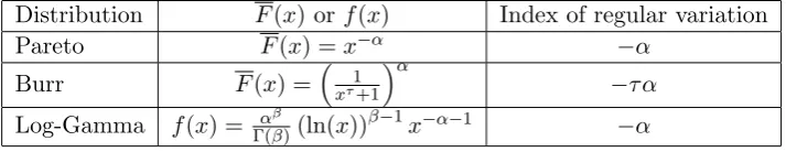
asymptotic mean squared error of the Hill estimator. Although it works very well for Pareto distributed data, for other regularly varying distribution functions the Hill estimator becomes less effective. To illustrate this we have drawn two different samples, one from the Pareto(1) distribution and one from a Burr distribution (see Table 4.1) with parameters such that the tail index of this Burr distribution is equal to one. Figure 1.8 (a), (b) shows the Hill estimator for the two data sets together with the 95%-confidence bounds of the estimate. Note that the Hill estimate is plotted against the different values in the data set running from largest to smallest.

and the largest value of the data set is plotted on the left of the x-axis. As we can see from

(16)

15 95 186 288 390 492 594 696 798 900

0.6

0.8

1.0

1.2

1.4

1.6

1.8

45.80 6.63 3.49 2.38 1.84 1.49 1.28 1.11

Order Statistics

alpha (CI, p =0.95)

Threshold

(a) Pareto distributed data

15 95 186 288 390 492 594 696 798 900

0.0

0.5

1.0

1.5

2.0

2.5

4.42e+01 1.17e+00 2.80e−01 7.29e−02 7.22e−03

Order Statistics

alpha (CI, p =0.95)

Threshold

[image:16.595.102.516.103.322.2]

(b) Burr distributed data

Figure 1.8: Hill estimator for samples of a Pareto and Burr distribution with tail index 1.

(a) Hill plot for crop loss (b) Hill plot for property damages from natural disas-ters

Figure 1.9: Hill estimator for crop loss and property damages from natural disasters

Figure 1.9, shows a Hill plot for crop losses (a) and natural disaster property damages (b). Figure 1.10 compares Hill plots for flood damages (a) and flood damages per income (b). The difference between these last two plots underscores the importance of properly accounting for exposure. Figure 1.9 (a) is more difficult to interpret than the mean excess plot in Figure (1.7)(b).

[image:16.595.93.539.363.605.2]

(17)

[image:17.595.65.510.87.313.2]

(a) Hill plot for flood claims (b) Hill plot for flood claims per income

Figure 1.10: Hill estimator for ﬂood claims

(a) Mean excess plot for hospital dis-charge bills

(b) Mean excess plot for hospital dis-charge bills, aggregation by 10

(c) Hill plot for hospital discharge bills

[image:17.595.135.434.344.706.2]

(18)

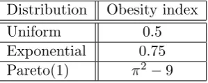
Distribution Obesity index

Uniform 0.5

Exponential 0.75

[image:18.595.238.388.88.148.2]

Pareto(1) π2−9

Table 1.2: Obesity index for a number of distributions

index in the neighborhood of 3. Although definitely heavy tailed according to all the operative definitions, it behaves like a distribution with finite variance, as we see the mean excess collapse under aggregation by 10.

(a) Mean excess plot for Gross Cell Product (non mineral)

[image:18.595.159.467.239.410.2]

(b) Hill plot for Gross Cell Product (non mineral)

Figure 1.12: Gross Cell Product (non mineral) obx=0.77

1.3.6 The Obesity Index

We have discussed two deﬁnitions of heavy-tailed distributions, the regularly varying

distribu-tions with tail index 0< α <∞ and subexponential distributions. Regularly varying

distribu-tions are a subset of subexponential distribudistribu-tions which have inﬁnite moments beyond a certain point, but subexponentials include distributions all of whose moments are ﬁnite (tail index

= ∞). Both deﬁnitions refer to limiting distributions as the value of the underlying variable

goes to infinity. In large finite data sets the diagnostics based on the mean excess plots can be quite similar. There is nothing like a ”degree of subexponentiality” allowing us to compare subexponential distributions with infinite tail index, and there is currently no characterization of obesity in finite data sets.

We therefore propose the following obesity index that is applicable to ﬁnite samples, and

which can be computed for distribution functions. Restricting the samples to the higher values then gives a tail obesity index.

Ob(X) =P(X1+X4> X2+X3|X1 ≤X2≤X3 ≤X4) ;

{X1, ...X4}independent and identically disributed.

In Table 1.2 the value of the Obesity index is given for a number of diﬀerent distributions. In

Figure 1.13 we see the Obesity index for the Pareto distribution, with tail indexα, and for the

Weibull distribution with shape parameterτ.

(19)

0 0.5 1 1.5 2 2.5 3 0.8

0.82 0.84 0.86 0.88 0.9 0.92 0.94 0.96 0.98 1

Tail Index

Obesity Index

(a) Pareto distribution

0 0.5 1 1.5 2 2.5 3 0.5

0.6 0.7 0.8 0.9 1

Shape Parameter

Obesity Index

[image:19.595.107.449.108.293.2]

(b) Weibull distribution

Figure 1.13: Obesity index for diﬀerent distributions.

distribution, ifτ <1; then the Weibull is a subexponential distribution and is considered

heavy-tailed. The Obesity index increases as τ decreases.

Given two random variablesX1 and X2 with tail indexes, α1 andα2,α1 < α2, the question

arises whether the Obesity index ofX1 larger than the Obesity index ofX2. Numerical

approxi-mation of two Burr distributed random variables indicate that this is not the case. ConsiderX1,

a Burr distributed random variable with parameters c = 1 and k = 2, and a Burr distributed

random variable with parametersc= 3.9 andk= 0.5. The tail index ofX1 is equal to 2 and the

tail index of X2 is equal to 1.95. But numerical approximation indicate that the Obesity index

of X1 is approximately equal to 0.8237 and the Obesity index ofX2 is approximately equal to

0.7463. Of course this should not come as a surprise; the obesity index in this case is applied to the whole distribution, whereas the tail index applies only to the tail.

A similar qualiﬁcation applies for any distributions taking positive and negative values. For

a symmetrical such as the normal or the Cauchy the Obesity index is always 1₂. The Cauchy

distribution is a regularly varying distribution with tail index 1 and the normal distribution is considered a thin-tailed distribution. In such cases it is more useful to apply the Obesity index separately to positive or negative values.

1.4 Conclusion and Overview of the Technical Chapters

Fat tailed phenomena are not rare or exotic, they occur rather frequently in loss data. As attested in hospital billing data and Gross Cell Product data, they are encountered in mundane economic data as well. Customary definitions in terms of limiting distributions, such as regular variation or subexponentiality, may have contributed to the belief that fat tails are mathematical freaks of no real importance to practitioners concerned with finite data sets. Good diagnostics help dispel this incautious belief, and sensitize us to the dangers of uncritically applying thin tailed statistical tools to fat tailed data: Historical averages, even in the absence of time trends may may be poor predictors, regardless of sample size. Aggregation may not reduce variation relative to the aggregate mean, and regression coefficients are based on ratios of quantities that fluctuate wildly.

(20)

1.4. CONCLUSION AND OVERVIEW OF THE TECHNICAL CHAPTERS 19

confounded by real or imagined time trends in the data. For heavy tailed data, the overall impression may be strongly affected by the ordering. Plotting different moving averages for different random orderings can be helpful. Mean excess plots provide a very useful diagnostic. Since these are based on ordered data, the problems of ordering do not arise. On the downside, they can be misleading for regular varying distributions with tail indices less than or equal to one, as the theoretical slope is infinite. Hill plots, though very popular, are often difficult to interpret. The Hill estimator is designed for regularly varying distributions, not for the wider class of subexponential distributions; but even for regularly varying distributions, it may be impossible to infer the tail index from the Hill plot.

In view of the jumble of diagnostics, each with their own strengths and weaknesses, it is useful to have an intuitive scalar measure of obesity, and the obesity index is proposed here for this purpose. The obesity index captures the idea that larger values are further apart, or that the sum of two samples is driven by the larger of the two, or again that the sum tends to behave like the max. This index does not require estimating a parameter of a hypothetical distribution; in can be computed for data sets and computed, in most cases numerically, for distribution functions.

(21)

(22)

Chapter 2 Order Statistics

This chapter discusses some properties of order statistic that are used later to derive properties of the Obesity index. Most of these properties can be found in David [1981] or Nezvorov [2001]. Another useful source is Balakrishnan and Stepanov [2007] We consider only order statistics from

an i.i.d. sequence of continuous random variables. Suppose we have a sequence ofnindependent

and identically distributed continuous random variablesX1, ..., Xn; if we order this sequence in

ascending order we obtain the order statistics

X1,n ≤...≤Xn,n.

2.1 Distribution of order statistics

In this section we derive the marginal and joint distribution of an order statistic. The distribution

function of ther-th order statisticXr,n, from a sample of a random variableX with distribution

functionF, is given by

Fr,n(x) = P(Xr,n≤x)

= P(at least r of the Xi are less than or equal to x)

=

n

∑

m=r

P( exactly mvariables among X1, ..., Xn ≤ x)

=

n

∑

m=r

(

n m

)

F(x)m(1−F(x))n−m

Using the following relationship for the regularized incomplete Beta function1

n

∑

m=k

(

n m

)

ym(1−y)n−m =

∫ y

0

n!

(k−1)!(n−k)!t

k−1₍₁₋_t₎n−k_dt, ₀_≤_y_≤₁_,

we get the following result

Fr,n(x) =IF(x)(r, n−r+ 1), (2.1)

whereIx(p, q) is the regularized incomplete beta function which is given by

Ix(p, q) =

1

B(p, q)

∫ x

0

tp−1(1−t)q−1dt,

1_{http://en.wikipedia.org/wiki/Beta function, accessed Feb.7 2011}

(23)

and B(p, q) is the beta function which is given by

B(p, q) =

∫ 1 0

tp−1(1−t)q−1dt.

Now assume that the random variable Xi has a probability density function f(x) = _dxdF(x).

Denote the density function of Xr,n withfr,n. Using (2.1) we get the following result.

fr,n(x) =

1

B(r, n−r+ 1)

d dx

∫ F(x) 0

tr−1(1−t)n−rdt,

= 1

B(r, n−r+ 1)F(x)

r−1₍₁₋_F₍_x₎₎n−r_f₍_x₎ _(2.2)

Where {k(1), ..., k(r)} is a subset of the numbers 1,2,3, ..., n, and k(0) = 0, k(r+ 1) = n+ 1 and ﬁnally 1≤r ≤n, the joint density ofX_k₍₁₎_,n, ..., X_k₍_r₎_,n is given by

fk(1),...,k(n);n(x1, ..., xr) =

n!

∏r+1

s=1(k(s)−k(s−1)−1)!

r_∏+1

s=1

(F(xs)−F(xs−1))k(s)−k(s−1)−1 r

∏

s=1

f(xs), (2.3)

where −∞ = x0 < x1 < ... < xr < xr+1 = ∞. We prove this for r = 2 and assume for

simplicity that f is continuous at the points x1 and x2 under consideration. Consider the

following probability

P(δ,∆) =P(x1 ≤Xk(1),n < x1+δ < x2 ≤Xk(2),n< x2+ ∆

)

.

We show that asδ →0 and ∆→0 the following limit holds.

f(x1, x2) = lim

P(δ,∆)

δ∆ Now deﬁne the following events

A = {x1≤Xk(1),n < x1+δ < x2≤Xk(2),n < x2+ ∆ and the intervals [x1, x1+δ) and [x2, x2+ ∆) each contain exactly one order statistic},

B = {x1≤Xk(1),n < x1+δ < x2≤Xk(2),n < x2+ ∆ and

[x1, x1+δ)∪[x2, x2+ ∆) contains at least three order statistics}.

We have thatP(δ,∆) =P(A) +P(B). Also deﬁne the following events

C = {at least two out of nvariables X1, ..., Xn fall into [x1, x1+δ)}

D = {at least two out of nvariables X1, ..., Xn fall into [x2, x2+ ∆)}.

Now we have that P(B)≤P(C) +P(D). We ﬁnd that

P(C) =

n

∑

k=2

(

n k

)

(F(x1+δ)−F(x1))k(1−F(x1+δ) +F(x1))n−k

≤ (F(x1+δ)−F(x1))2

n

∑

k=2

(

n k

)

≤ 2n(F(x1+δ)−F(x1))2

(24)

2.2. CONDITIONAL DISTRIBUTION 23

and similarly we obtain that

P(D) =

n

∑

k=2

(

n k

)

(F(x2+ ∆)−F(x2))k(1−F(x2+ ∆) +F(x2))n−k

≤ (F(x2+ ∆))

n

∑

k=2

(

n k

)

≤ 2n(F(x2+ ∆)−F(x2))2

= O(∆2), ∆→0.

This yields

limP(δ,∆)−P(A)

δ∆ = 0 asδ →0, ∆→0.

It remains to note that

P(A) = n!

(k(1)−1)!(k(2)−k(1)−1)!(n−k(2))!F(x1)

k(1)−1₍_F₍_x

1+δ)−F(x1))

(F(x2)−F(x1+δ))k(2)−k(1)−1(F(x2+ ∆)−F(x2)) (1−F(x2))n−k(2).

From this equality we see that the limit exists and that

f(x1, x2) =

n!

(k(1)−1)!(k(2)−k(1)−1)!(n−k(2))!F(x1)

k(1)−1₍_F₍_x₂₎₋_F₍_x₁₎₎k(2)−k(1)−1

(1−F(x2))n−k(2)f(x1)f(x2),

which is the same as the joint distribution we wrote down earlier. Note that we have only found

the right limit of f(x1 + 0, x2 + 0), but since f is continuous we can obtain the other limits

f(x1+ 0, x2−0), f(x1−0, x2+ 0) andf(x1−0, x2−0) in a similar way.

Also note that when r = n in (2.3) we get the joint density of all order statistics and that

this joint density is given by

f1,...,n;n(x1, ..., xn) =

{

n!∏n_s₌₁f(xs) if, − ∞< x1< ... < xn<∞

0, otherwise. (2.4)

2.2 Conditional distribution

When we pass from the original random variables X1, ..., Xn to the order statistics, we lose

independence among these variables. Now suppose we have a sequence of n order statistics

X1,n, ..., Xn,n, and let 1< k < n. In this section we derive the distribution of an order statistic

Xk+1,ngiven the previous order statisticXk=xk, ..., X1 =x1. Let the density of this conditional

(25)

distribution of Xk+1,n given thatXk,n=xk, denoted byf(u|xk)

f(u|x1, ..., xk) =

f1,...,k+1;n(x1, ..., xk, u)

f1,...,k;n(x1, ..., xk)

=

n!

(n−k−1)![1−F(u)]

n−k−1∏k

s=1f(xs)f(u) n!

(n−k)![1−F(xk)]

n−k∏k

s=1f(xs)

=

n!

(k−1)!(n−k−1)![1−F(u)]

n−k−1_F₍_x

k)k−1f(xk)f(u) n!

(k−1)!(n−k)![1−F(xk)]

n−k

F(xk)k−1f(xk)

= fk,k+1;n(xk, u)

fk,n(xk)

=f(u|xk).

From this we see that the order statistics form a Markov chain. The following theorem is useful for ﬁnding the distribution of functions of order statistics.

Theorem 2.2.1. Let X1,n ≤...≤Xn,n be order statistics corresponding to a continuous

distri-bution function F. Then for any 1< k < n the random vectors

X(1) = (X1,n, ..., Xk−1,n) and X(2)= (Xk+1,n, ..., Xn,n)

are conditionally independent given any fixed value of the order statistic Xk,n. Furthermore,

the conditional distribution of the vector X(1) given that Xk,n = u coincides with the

uncondi-tional distribution of order statisticsY1,k−1, ..., Yk−1,k−1 corresponding to i.i.d. random variables

Y1, ..., Yk−1 with distribution function

F(u)(x) = F(x)

F(u) x < u.

Similarly, the conditional distribution of the vectorX(2) givenXk,n =ucoincides with the

uncon-ditional distribution of order statistics W1,n−k, ..., Wn−k;n−k related to the distribution function

F(u)(x) =

F(x)−F(u)

1−F(u) x > u.

Proof. To simplify the proof we assume that the underlying random variables X1, ..., Xn have

densityf. The conditional density is given by

f(x1, ..., xk−1, xk+1, ..., xn|Xk,n=u) =

f1,...,n;n(x1, ..., xk−1, xk+1,n, ..., xn)

fk;n(u)

=

[

(k−1)!

k_∏−1

s=1

f(xs)

F(u)

] [

(n−k)!

n

∏

r=k+1

f(xr)

1−F(u)

]

.

As we can see the ﬁrst part of the conditional density is the joint density of the order statistics from a sample sizek−1 where the random variables have a density _Ff(₍x_u)₎ forx < u. The second

part in the density is the joint density of the order statistics from a sample of sizen−kwhere

(26)

2.3. REPRESENTATIONS FOR ORDER STATISTICS 25

2.3 Representations for order statistics

We noted that one of the drawbacks of using the order statistics is losing the independence property among the random variables. If we consider order statistics from the exponential distribution or the uniform distribution there are a few useful properties of the order statistics that can be used when studying linear combinations of the order statistics.

Theorem 2.3.1. Let X1,n ≤... ≤Xn,n, n= 1,2, ..., be order statistics related to independent

and identically distributed random variables with distribution functionF, and let

U1,n ≤...≤Un,n,

be order statistics related to a sample from the uniform distribution on [0,1]. Then for any

n= 1,2, ... the vectors (F(X1,n), ..., F(Xn,n)) and(U1,n, ..., Un,n) are equally distributed.

Theorem 2.3.2. Consider exponential order statistics

Z1,n ≤...≤Zn,n,

related to a sequence of independent and identically distributed random variables Z1, Z2, ... with

distribution function

H(x) = max(0,1−e−x).

Then for any n= 1,2, ... we have

(Z1,n, ..., Zn,n) d

=

(

v1

n, v1

n + v2

n−1, ...,

v1

n +...+vn

)

, (2.5)

where v1, v2, ... is a sequence of independent and identically distributed random variables with

distribution function H(x).

Proof. In order to prove Theorem 2.3.2 it suﬃces to show that the densities of both vectors in (2.5) are equal. Putting

f(x) =

{

e−x, ifx >0,

0 otherwise, (2.6)

and substituting equation (2.6) into the joint density of thenorder statistics given by

f1,2,...,n;n(x1, ..., xn) =

{

n!∏n_i₌₁f(xi), x1 < ... < xn,

0, otherwise,

we ﬁnd that the joint density of the vector on the LHS of equation (2.5) is given by

f1,2,...,n;n(x1, ..., xn) =

{

n! exp{−∑n_s₌₁xs}, if 0< x1 < ... < xn<∞,

0, otherwise. (2.7)

The joint density ofn i.i.d. standard exponential random variablesv1, ..., vn is given by

g(y1, ..., yn) =

{

exp{−∑n_s₌₁ys}, ify1>0, ..., yn>0,

0, otherwise. (2.8)

The linear change of variables

(v1, ..., vn) = (

y1

n, y1

n + y2

n−1,

y1

n + y2

n−1 +

y3

n−2, ...,

y1

(27)

with Jacobian _n_! which corresponds to the passage to random variables

V1=

v1

n, V2 = v1

n + v2

n−1, ..., Vn=

v1

n +...+vn,

has the property that

v1+v2+...+vn=y1+...+yn

and maps the domain{ys>0s= 1, ..., n}into the domain{0< v1 < v2 < ... < vn<∞}.

Equa-tion (2.8) implies that V1, ..., Vn have the joint density

f(v1, ..., vn) =

{

n! exp{−∑n_s₌₁vs}, if 0< v1< ... < vn,

0, otherwise. (2.9)

Comparing equation (2.7) with equation (2.9) we ﬁnd that both vectors in (2.5) have the same density and this proves the theorem.

Using Theorem 2.3.2 it is possible to ﬁnd the distribution of any linear combination of order statistics from an exponential distribution, since we can express this linear combination as a sum of independent exponential distributed random variables.

Theorem 2.3.3. Let U1,n ≤...≤Un,n,n= 1,2, ... be order statistics from an uniform sample.

Then for any n= 1,2, ...

(U1,n, ..., Un,n) d

=

(

S1

Sn+1

, ..., Sn Sn+1

)

,

where

Sm =v1+...+vm, m= 1,2, ...,

and where v1, ..., vm are independent standard exponential random variables.

2.4 Functions of order statistics

In this section we discuss diﬀerent techniques that can be used to obtain the distribution of diﬀerent functions of order statistics.

2.4.1 Partial sums

Using Theorem 2.2.1 we can obtain the distribution of sums of consecutive order statistics,

∑s−1

i=r+1Xi,n. The distribution of the order statistics Xr+1,n, ..., Xs−1,n given that Xr,n = y and Xs,n = z coincides with the unconditional distribution of order statistics V1,n, ..., Vs−r−1 corresponding to an i.i.d. sequenceV1, ..., Vs−r−1 where the distribution function of Vi is given

by

Vy,z(x) =

F(x)−F(y)

F(z)−F(y), y < x < z. (2.10) From Theorem 2.2.1 we can write the distribution function of the partial sum in the following way

P(Xr+1+...+Xs−1 < x) =

∫

−∞<y<z<∞

P(Xr+1+...+Xs−1 < x|Xr,n=y, Xs,n=z)fr,s;n(y, z)dydz

=

∫

−∞<y<z<∞

V_y,z(s−r−1)∗(x)fr,s;n(y, z)dydz,

(28)

2.4. FUNCTIONS OF ORDER STATISTICS 27

2.4.2 Ratio between order statistics

Now we look at the distribution of the ratio between two order statistics.

Theorem 2.4.1. Forr < s and0≤x≤1

P

(

Xr,n

Xs,n ≤

x

)

= 1

B(s, n−s+ 1)

∫ 1 0

IQx(t)(r, s−r)t

s−1₍₁₋_t₎n−s_dt, _(2.11)

where

Qx(t) =

F(xF−1(t))

t .

Proof.

P

(

Xr,n

Xs,n ≤

x ) = ∫ _∞ −∞P ( y Xs,n ≤

x|Xr,n=y

)

fXr,n(y)dy,

=

∫ _∞

−∞P

(

Xs,n>

y

x|Xr,n=y

)

fXr,n(y)dy,

= ∫ _∞ −∞ ∫ _∞ y x

f_X_s,n_|_X_r,n₌_y(z)dzfXr,n(y)dy,

=

∫ _∞

−∞

∫ zx

−∞fXr,n(y)fXs,n|Xr,n=y(z)dydz,

= C

∫ _∞

−∞

∫ zx

−∞F(y)

r−1_[1₋_F₍_y_)]n−r_f₍_y₎

[F(z)−F(y)]s−r−1[1−F(z)]n−sf(z) [1−F(y)]n−r dydz,

where C = _B₍_r,n₋_r₊₁₎_B1₍_s₋_r,n₋_s₊₁₎. We apply the transformation t = F(z) from which we get the following

P

(

Xr,n

Xs,n ≤

x

)

= C

∫ 1 0

∫ xF−1₍_t₎

−∞ F(y)

r−1_f₍_y_{) [}_t₋_F₍_y_)]s−r−1_dy₍₁₋_t₎n−s_dt.

Next we use the transformation F(_ty) =u.

P

(

Xr,n

Xs,n ≤

x

)

= C

∫ 1 0

∫ F(xF−1(t))

t

0

tr−1ur−1(t−tu)s−r−1tdu(1−t)n−sdt,

= C

∫ 1 0

∫ F(xF−1(t))

t

0

ur−1(1−u)s−r−1duts−1(1−t)n−sdt

We can rewrite the constantC in the following way

C = 1

B(r, n−r+ 1)B(s−r, n−s+ 1)

= n!

(r−1)!(n−r)!

(n−r)! (s−r−1)!(n−s)!

= 1

(s−r−1)!(r−1)!

n! (n−s)!

= (s−1)!

(s−r−1)!(r−1)!

n! (n−s)!(s−1)!

= 1

(29)

If we substitute this in our integral, and deﬁneQx(t) = _t , we get the following

P

(

Xr,n

Xs,n ≤

x

)

= 1

B(s, n−s+ 1)

∫ 1 0

∫Qx(t)

0 u

r−1₍₁₋_u₎s−r−1_du

B(s, s−r) t

s−1₍₁₋_t₎n−s_dt

= 1

B(s, n−s+ 1)

∫ 1 0

IQx(t)(r, s−r)t

s−1₍₁₋_t₎n−s

dt.

(30)

Chapter 3 Records

Records are used in Chapter 5 to explore possible measures of tail obesity. Records are closely related to order statistics. This brief chapter discusses the theory of records and summarizes the main results. For a more detailed discussion see Arnold [1983],Arnold et al. [1998] or Nezvorov [2001], where most of the results we present here can be found. Records are closely related to extreme values and related material can be found in A.J. McNeil and Embrechts [2005], Coles [2001]and Beirlant et al. [2005].

3.1 Standard record value processes

Let X1, X2, ... be an inﬁnite sequence of independent and identically distributed random

vari-ables. Denote the cumulative distribution function of these random variables byF and assume

it is continuous. An observation is called an upper record value if its value exceeds all previous observations. SoXj is an upper record if Xj > Xi for alli < j. We are also interested in the

times at which the record values occur. For convenience assume that we observeXj at time j.

The record time sequence{Tn, n≥0}is deﬁned as

T0= 1 with probability 1

and forn≥1,

Tn= min

{

j:Xj > XTn−1

}

.

The record value sequence{Rn} is then deﬁned by

Rn=XTn, n= 0,1,2, ...

The number of records observed at time n is called the record counting process {Nn, n ≥ 1}

where

Nn={number of records amongX1, ..., Xn}.

We have thatN1 = 1 sinceX1 is always a record.

3.2 Distribution of record values

Let the record increment process be deﬁned by

Jn=Rn−Rn−1, n >1,

withJ0 =R0. It can easily be shown that if we consider the record increment process from a

sequence of i.i.d. standard exponential random variables then all the Jn are independent and

(31)

Jn has a standard exponential distribution. Using the record increment process we are able

to derive the distribution of the n-th record from a sequence of i.i.d. standard exponential

distributed random variables.

P(Rn< x) = P(Rn−Rn−1+Rn−1−Rn−2+Rn−2−...+R1−R0+R0 < x) = P(Jn+Jn−1+...+J0< x)

Since∑n_i₌₀J+iis the sum ofn+ 1 standard exponential distributed random variables we ﬁnd

that the record values from a sequence of standard exponential distributed random variables

has the gamma distribution with parameters n+ 1 and 1.

Rn∼Gamma(n+ 1,1), n= 0,1,2, ...

If a random variableXhas a Gamma(n, λ) distribution then it has the following density function

fX(x) =

{_λ₍_λx₎n−1_e−λx

Γ(n) , x≥0

0, otherwise

We can use the result above to ﬁnd the distribution of the n-th record corresponding to a

sequence {Xi} of i.i.d. random variables with continuous distribution function F. If X has

distribution functionF then

H(X)≡ −log(1−F(X))

has a standard exponential distribution function. We also have thatX=d F−1(1−e−X∗) where

X∗ is a standard exponential random variable. Since X is a monotone function of X∗ we can

express the n-th record of the sequence {Xj} as a simple function of the n-th record of the

sequence {X∗}. This can be done in the following way

Rn d

=F−1(1−e−Rn∗₎_, _n_{= 0}_,₁_,₂_{, ...}

Using the following expression of the distribution of then-th record from a standard exponential

sequence

P(R_n∗ > r∗) =e−r∗

n

∑

k=0 (r∗)k

k! , r ∗_>₀_,

the survival function of the record from an arbitrary sequence of i.i.d. random variables with

distribution functionF is given by

P(Rn> r) = [1−F(r)] n

∑

k=0

−[log(1−F(r))]k

k! .

3.3 Record times and related statistics

The deﬁnition of the record time sequence{Tn, n≥0}was given by

T0 = 1, with probability 1,

and for n≥1

(32)

3.3. RECORD TIMES AND RELATED STATISTICS 31

In order to find the distribution of the firstnnon-trivial record timesT1, T2, ..., Tnwe first look

at the sequence of record time indicator random variables. These are deﬁned in the following way

I1 = 1 with probability 1, and forn >1

In=1_{Xn>max{X1,...,Xn−1}}

So In = 1 if and only if Xn is a record value. We assume that the distribution function F, of

the random variables we consider, is continuous. It is easily veriﬁed that the random variables

Inhave a Bernoulli distribution with parameter 1_n and are independent of each other. The joint

distribution for the ﬁrstmrecord times can be obtained using the record indicators. For integers

1< n1 < ... < nm we have that

P(T1 =n1, ..., Tm =nm) =P(I2 = 0, ..., In1−1= 0, In1 = 1, In1+1 = 0, ..., Inm = 0)

= [(n1−1)(n2−1)...(nm−1)nm]−1.

In order to ﬁnd the marginal distribution of Tk we ﬁrst review some properties of the record

counting process{Nn, n≥1} deﬁned by

Nn={number of records amongX1, ...Xn}

=

n

∑

j=1

Ij.

Since the record indicators are independent we can immediately write down the mean and the variance forNn.

E[Nn] = n

∑

j=1 1

j,

Var(Nn) = n

∑

j=1 1

j

(

1−1

j

)

.

We can obtain the exact distribution ofNn using the probability generating function. We have

the following result.

E[sNn]₌ n

∏

j=1

E[sIj]

=

n

∏

j=1

(

1 +s−1

j

)

From this we ﬁnd that

P(Nn=k) =

Sk n

n!

whereS_nk is a Stirling number of the ﬁrst kind. The Stirling numbers of the ﬁrst kind are given

by the coeﬃcients in the following expansion .

(x)n= n

∑

k=0

Heavy-tailed distributions : data, diagnostics, and new developments

Heavy-Tailed

Distributions: Data,

Diagnostics, and New

Developments

Heavy-Tailed Distributions:

Data, Diagnostics and New Developments

Contents

Chapter 1

Fatness of Tail

1.1

Fat tail heuristics

1.2

History and Data

1.3

Diagnostics for Heavy Tailed Phenomena

1.4

Conclusion and Overview of the Technical Chapters

Chapter 2

Order Statistics

2.1

Distribution of order statistics

2.2

Conditional distribution

2.3

Representations for order statistics

2.4

Functions of order statistics

Chapter 3

Records

3.1

Standard record value processes

3.2

Distribution of record values

3.3

Record times and related statistics