Modeling thermocapillary migration of a microfluidic
droplet on a solid surface
Haihu Liu∗, Yonghao Zhang
James Weir Fluids Laboratory, Department of Mechanical & Aerospace Engineering, University of Strathclyde, Glasgow G1 1XJ, UK
Abstract
A multiphase lattice Boltzmann model is developed to simulate immiscible thermocapillary flows with the presence of fluid-surface interactions. In this model, interfacial tension force and Marangoni stress are included by intro-ducing a body force term based on the concept of continuum surface force, and phase segregation is achieved using the recoloring algorithm proposed by Latva-Kokko and Rothman. At a solid surface, fluid-surface interactions are modeled by a partial wetting boundary condition that uses a geometric formulation to specify the contact angle, and a color-conserving boundary closure scheme to improve the numerical accuracy and suppress spurious ve-locities at the contact line. An additional convection-diffusion equation is solved by the passive scalar approach to obtain the temperature field, which is coupled to the hydrodynamic equations through an equation of state. This model is first validated by simulations of static contact angle and dynamic capillary intrusion process when a constant interfacial tension is considered. It is then used to simulate the thermocapillary migration of a microfluidic droplet on a horizontal solid surface subject to a uniform temperature gra-dient. We for the first time demonstrate numerically that the droplet mo-tion undergoes two different states depending on the surface wettability: the droplet migrates towards the cooler regions on hydrophilic surfaces but re-verses on hydrophobic surfaces. Decreasing the viscosity ratio can enhance the intensity of thermocapillary vortices, leading to an increase in migration velocity. The contact angle hysteresis, i.e., the difference between the
advanc-∗Corresponding author
ing and receding contact angles, is always positive regardless of the contact angle and viscosity ratio. The contact angle hysteresis and the migration velocity both first decreases and then increases with the contact angle, and their minimum values occur at the contact angle of 90 degrees.
Keywords:
Thermocapillary migration, Lattice Boltzmann method, Multiphase flow, Wetting boundary condition, Microfluidics, Droplet dynamics
1. Introduction
Thermocapillary convection is a phenomenon of fluid movement that arises as a consequence of the variation of interfacial tension at a fluid-fluid interface caused by temperature gradients. It has been known as a mecha-nism for driving the motion of droplets and bubbles immersed in a second fluid since the pioneering work of Young et al. [1]. For most fluids inter-facial tension is a decreasing function of temperature, and this leads to the movement of droplets or bubbles suspended in a bulk fluid from the regions of lower temperature to the warmer regions; such a subject has been studied ex-tensively due to its importance in space material processing and many other engineering and scientific applications under microgravity conditions where sedimentation and gravity-driven convection are largely eliminated [2]. Over the last decade or so, attention has been focused on using thermocapillary forces to manipulate the motion and dynamic behavior of droplets or bub-bles in microfluidic devices, where bulk phenomena can be negligible in com-parison with interfacial effects due to large surface-to-volume ratio and low Reynolds number. Thermocapillary actuation is advantageous over convec-tional hydrodynamic stress, electrohydrodynamic force, and magnetic force methods for droplet and bubble manipulations, as it can be generated eas-ily by means of substrate embedded microheaters [3, 4] or by localized laser heating [5, 6] that allows contactless, reconfigurable, and real-time control of multiple droplets without the need for any special microfabrication or moving parts. To date, the thermocapillary force has been combined with geome-try of the microchannel to realise various droplet manipulations including mixing, sorting, fission, fusion, sampling and switching [7, 8].
of channel walls would quantitatively or qualitatively modify the physics of thermocapillary migration in a microfluidic channel [5, 9]. For example, it was observed that a liquid droplet placed on a horizontal solid surface can move toward cooler regions [10], as opposed to that in an unbounded flow condition. There have been a number of experimental studies investigating the migration of a liquid droplet on a solid surface induced by thermal gra-dients [11, 12, 13, 14, 15]. However, it is still very difficult to conduct precise experimental measurements of the local temperature and flow fields during the migration process of a droplet. Theoretical studies based on a lubrica-tion approximalubrica-tion have been used for analyzing the migralubrica-tion velocity of a droplet with sufficiently small aspect ratio (defined by the maximum height of the droplet to its length) induced by thermocapillary force [16, 17, 10, 18]. Unfortunately, they are unable to solve the transient thermocapillary migra-tion of a spherical cap droplet with a large contact angle due to the limitamigra-tion of lubrication approximation. Numerical modelling and simulations can com-plement theoretical and experimental studies, providing an efficient pathway to enhance our understanding of thermocapillary migration of droplets in a microchannel.
are due to interparticle interactions [26]. Thus, mesoscopic level models are expected to describe more accurately the multiscale thermocapillary flows in a confined microfluidic device.
The lattice Boltzmann (LB) method has become a promising alternative to traditional CFD methods for simulating complex fluid flow problems. It is a pseudo-molecular method based on particle distribution functions that per-forms microscopic operations with mesoscopic kinetic equations and repro-duces macroscopic behavior [27]. Its mesoscopic kinetic nature offers many of the advantages of molecular dynamics, making LB method particularly suited for modeling multiphase, multicomponent flows. A number of multiphase, multicomponent models have been proposed in the LB community, which can be classified into four major types: color-fluid model [28, 29, 30, 31], phase-field-based model [32, 33, 34], interparticle-potential model [35, 36, 37], and mean-field theory model [38]. These models have shown great success in mod-eling multiphase flow problems with a constant interfacial tension [39]. Based on the color-fluid model, we recently proposed the first LB model to simu-late thermocapillary flows, through which we first numerically demonstrate that the micro-droplet manipulation can be achieved through the thermo-capillary forces induced by the laser heating [40]. Later, we developed two phase-field-based thermocapillary models with one focusing on high-density-ratio two-phase flows [41] and the other on modeling fluid-surface interac-tions [9]. Although the thermocapillary color-fluid model inherits a series of advantages of the model by Halliday and his coworkers [42, 29], such as low spurious velocities, high numerical accuracy and strict mass conserva-tion for each fluid, it can only simulate thermocapillary flows with droplets suspended in a carrier fluid, away from the wall boundary.
applied to improve the numerical accuracy and suppress spurious currents at the contact line. The capability and accuracy of this model are first tested by two benchmark cases with analytical solutions. It is then used to simulate the thermocapillary migration of a microfluidic droplet adhering on a hori-zontal solid surface subject to a uniform temperature gradient, in which the influence of contact angle and fluid viscosity ratio on the droplet migration are systematically investigated.
2. Methodology
2.1. Color-fluid lattice Boltzmann model for thermocapillary flow
A color-fluid LB model was recently developed by Liu et al. [40] to simu-late thermocapillary flows. In this model, red and blue distribution functions
fR
i and fiB are introduced to represent two different fluids, and the total dis-tribution function is defined as: fi = fiR +fiB. Each of the colored fluids undergoes the collision and streaming operations:
fik(x+eiδt, t+δt) = fik(x, t) + Ω k
i(x, t), (1) where the superscript k = R or B denotes the color (“Red” or “Blue”),
fi(x, t) is the distribution function in the i-th velocity direction at the posi-tion xand time t, ei is the lattice velocity in thei-th direction,δt is the time step, and Ωk
i is the collision operator. The collision operator is the result of the combination of three sub-operators [31]:
Ωki = (Ω k i)(3)
(Ωki)(1)+ (Ω k i)(2)
, (2)
where (Ωk
i)(1)is the Bhatnagar-Gross-Krook (BGK) collision operator, (Ωki)(2) is the two-phase collision operator which contributes to the mixed interfacial region and generates an interfacial force, and (Ωk
i)(3)represents the recoloring operator which mimics the phase segregation and keeps the interface sharp.
The BGK collision operator is given by (Ωki)(1) =−
1
τf
fik−f k,eq i
, (3)
where τf is the dimensionless relaxation time, and fik,eq is the equilibrium distribution function of fk
i. Conservation of mass for each fluid and total momentum conservation require
ρk =
X
i
fik =
X
i
ρu =X k
X
i
fikei =
X
k
X
i
fik,eqei, (5)
where ρk is the density of fluid k,ρ=ρR+ρB is the total density andu the local fluid velocity. For the two-dimensional 9-velocity (D2Q9) model [49], the lattice velocity ei is defined as e0 = (0,0), e1,3 = (±c,0), e2,4 = (0,±c), e5,7 = (±c,±c), ande6,8 = (∓c,±c), wherec=δx/δt is the lattice speed and
δx the lattice spacing. The equilibrium distribution functions are chosen to respect the conservation constraints of Eqs. (4) and (5)
fik,eq(ρk,u) =ρkwi
1 + ei·u
c2
s
+ (ei·u)
2
2c4
s
− u
2
2c2
s
, (6)
wherecs= 1/
√
3cis the lattice sound speed, andwi is the weight factor with
w0 = 4/9, w1−4 = 1/9 andw5−8 = 1/36.
An indicator functionρN is introduced to identify the location of interface, and is defined by
ρN(x, t) = ρr(x, t)−ρb(x, t)
ρr(x, t) +ρb(x, t), −1≤ρ N
≤1. (7)
In the LBM community, the concept of continuum surface force (CSF) was first used by Lishchuk et al. [42] to model the interfacial force with constant interfacial tension, which was demonstrated to effectively reduce the spurious velocities. It was later extended by Liu and Zhang [40] to model the interfacial force with temperature-dependent interfacial tension and Marangoni stress. Following Liu and Zhang, the interfacial force reads as
F(x, t) = 1 2|∇ρ
N
|(σκn+∇sσ), (8) whereIis the second-order identity tensor,∇s= (I−n⊗n)·∇is the surface gradient operator,σis the interfacial tension, nis the interfacial unit normal vector defined by
n= ∇ρ N
|∇ρN|, (9)
and κ is is the local interface curvature related to n by
In a thermocapillary flow, an equation of state is needed to relate the interfacial tension to the temperature, which may be linear or nonlinear. For the sake of simplicity, we only consider a linear relation between the interfacial tension and the temperature, i.e.,
σ(T) =σref +σT(T −Tref), (11) whereσref is the interfacial tension at the reference temperatureTref andσT is the interfacial tension gradient with respect to temperature.
Substituting of Eqs. (9) and (11) into Eq. (8), we obtain the interfacial force as
F(x, t) = 1 2σκ∇ρ
N +1
2σT|∇ρ N
|(I−n⊗n)· ∇T. (12) The interfacial force is then incorporated into LBM through the body force model of Guo et al. [50] because of its high accuracy in modeling a spatially varying body force and capability in reducing effectively the spuri-ous velocities [29, 46]. According to Guo et al. [50], the two-phase collision operator (Ωk
i)(2) is written as (Ωki)(2) =Ak
1− 1 2τf
ωi
ei−u
c2
s
+ei·u
c4
s
ei
·F, (13) where the free parameterAksatisfies
P
kAk= 1, and the velocity is redefined to include some of the effect of external body force [50]
ρu =X k
X
i
fikei+ 1
2Fδt. (14)
Using the Chapman-Enskog multiscale analysis, Eq. (1) can be reduced to the Navier-Stokes equations in the low frequency, long wavelength limit with Eqs. (3), (6), (13) and (14). The resulting equations are
∂tρ+∇ ·(ρu) = 0, (15)
∂t(ρu) +∇ ·(ρuu) =−∇p+∇ ·[ρν(∇u+∇uT)] +F, (16) wherep=ρc2
s is the pressure, andν =c2s(τf−12)δt is the kinematic viscosity of the fluid mixture. To account for unequal viscosities of the two fluids, the following function is used to determine the viscosity of the fluid mixture [51]
1
ν =
1 +ρN 2νR
+1−ρ N
2νB
or 1
τ −0.5 =
1 +ρN 2(τR−0.5)
+ 1−ρ N
2(τB−0.5)
where νk (k =R or B) is the kinematic viscosity of fluid k, which is related to the dimensionless relaxation time τk as νk = c2s(τk − 12)δt. It has been demonstrated that the choice of Eq. (17) can ensure the continuity of viscosity flux across the interface [51].
To minimize the discretization errors, the derivatives in Eq. (12) are eval-uated numerically through the nine-point isotropic finite difference stencils for a variable ψ [31]:
∇ψ(x, t) = 1
c2
s
X
i
wiψ(x+eiδt, t)ei. (18)
Although the two-phase collision operator generates the interfacial ten-sion and Marangoni stress, it does not guarantee the immiscibility of both fluids. To promote phase segregation and maintain the interface, the recolor-ing algorithm proposed by Latva-Kokko and Rothman [44] is applied. This algorithm allows the red and blue fluids to mix moderately at the tangent of the interface, and at the same time keeps the color distribution symmetric with respect to the color gradient. Thus, it helps further reduce the spurious velocities and removes the lattice pinning problem produced by the original recoloring algorithm of Gunstensen et al. [52]. In addition, compared to the recoloring algorithm of Gunstensen et al., it greatly increases the rate of convergence, improves the numerical stability and accu-racy of the solutions over a broad range of model parameters [52].
Following Latva-Kokko and Rothman [44], the recoloring operators for the red and blue fluids are defined by
(ΩR i )
(3)(fR i ) =
ρR
ρ f †
i +β
ρRρB
ρ wi|ei|cos(ϕi),
(ΩBi )(3)(f B i ) =
ρB
ρ f †
i −β
ρRρB
ρ wi|ei|cos(ϕi),
(19)
where fi† denotes the total distribution function after the two-phase colli-sion. β is the segregation parameter and is fixed at 0.7 to maintain a narrow interface thickness and reduce spurious velocities [53]; several recent stud-ies [54, 31] also showed that this choice is necessary to reproduce correct interface dynamics. ϕi is the angle between the indicator function gradient
∇ρN and the lattice vector ei, which is defined by cos(ϕi) = ei · ∇ρ
N
|ei||∇ρN|
To model the temperature field evolution, another particle distribution function gi is used, with the governing equation [45, 40]
gi(x+eiδt, t+δt)−gi(x, t) =− 1
τg
[gi(x, t)−gieq(x, t)], (21) where τg is the relaxation parameter, andg
eq
i is the equilibrium distribution function
gieq =T ωi
1 + ei·u
c2
s
+(ei·u)
2
2c4
s
− u
2
2c2
s
, (22)
whereT is the temperature. With the macroscopic velocity given by Eq. (14), Eq. (21) can recover the following convection-diffusion equation
∂tT +u· ∇T =∇ ·(κ∇T), (23) where κ = (τg − 12)c2sδt is the thermal conductivity. Following the definition of fluid viscosity given by Eq. (17), we define the thermal conductivity of mixture as
1
κ =
1 +ρN 2κR
+1−ρ N
2κB
, (24)
where κR (κB) is the thermal conductivity of red (blue) fluid. 2.2. Wetting boundary condition
To model fluid-surface interactions, our recently developed wetting bound-ary condition (WBC) [46] is adopted because of its advantages in modeling the contact line dynamics such as high accuracy and small spurious velocities. In the WBC, a constant (microscale) contact angle is prescribed at the solid surface, which is assumed to be equal to the equilibrium contact angle θeq, as done by Ding and Spelt [47, 55]. The contact
angle is enforced by using the geometrical properties of the indicator func-tion ρN at the contact line, a color-conserving boundary closure scheme [48] is applied to ensure mass conservation for each fluid, and a variant of the recoloring operator is designed to maintain the reasonable interface at the solid boundary.
Assuming that the contours of the indicator function in the diffuse inter-face are approximately parallel to each other, the equilibrium contact angle
θeq can be calculated geometrically in terms ofρN by [47] tanπ
2 −θ
eq= −nw· ∇ρN
|∇ρN −(n
w· ∇ρN)nw|
= −nw· ∇ρ N
|(tw· ∇ρN)tw|
1 2
3
5
4 6
7 8
unknown fiR, fiB
known fiR, fiB
0
wall (uw,vw)
Figure 1: (Color online) Illustration of a D2Q9 lattice node on the bottom wall of a two-dimensional domain after the propagation step. The wall is supposed to move with the velocityuw= (uw, vw). The fluid and solid are represented by the white and grey regions,
respectively.
where nw is the unit normal vector to wall pointing towards the fluid, and
tw is the unit vector tangential to wall. From Eq. (25), one has
nw· ∇ρN =−Θw|tw· ∇ρN|, (26) with
Θw = tanπ 2 −θ
eq
. (27)
In the present algorithm, the tangential component of∇ρN is determined by the central difference approximation. Then, the normal component of ∇ρN is obtained using Eq. (26). Thus, the contact angle is implicitly imposed by the gradient of indicator function at the solid wall.
The color-conserving boundary closure scheme [48] is employed to de-termine appropriate distribution functions for live links after the two-phase collision. Fig. 1 depicts a lattice node on the bottom wall, which moves at a velocity ofuw = (uw, vw). Assume that the node lies in the interface between the red and blue fluids. At this lattice node, the post-propagation value of distribution function fk
i exists only for i 6= 2,5,6, thus, the total of distri-bution functions that propagate into the fluid domain at the node depicted for each fluid is given by %k
in =
P
i6=2,5,6fik. After the two-phase collision, the distribution functions need to be considered only for live links, i.e., i6= 4,7,8 since the distribution functions withi= 4,7,8 will propagate out of the fluid domain after the propagation. Therefore, the effective mass for each fluid af-ter two-phase collision is given as P
i6=4,7,8f
k†
i . To ensure mass conservation for each fluid during the collision, it requires that,
X
i6=4,7,8
fik†=%k
[image:10.612.220.391.74.156.2]According to Eq. (1), the distribution function for the fluid k after the two-phase collision can be written as
fik† =f k,eq i (ρ
∗
k,uw) + (Ω k i)(2)+
1− 1
τf
fik(1), (29)
where fik(1) =fik−f k,eq
i denotes the higher-order component of the distribu-tion funcdistribu-tion fk
i, and ρ∗k is an auxiliary boundary density. The subtotal of
fik(1)on the live links is assumed to be zero, and the subtotal of the two-phase collision operator on the live links disrupts the conservation by
∆Mk=
X
i6=4,7,8
(Ωk i)
(2) = X
i6=4,7,8
Ak
1− 1 2τf
ωi
ei−u
c2
s
+ei·u
c4
s
ei
·F6= 0.
(30) By substituting of Eqs. (29) and (30) into Eq. (28), the auxiliary boundary density is obtained
ρ∗k =
%k
in−∆Mk
P
i6=4,7,8f
k,eq
i (1,uw) = %
k
in−∆Mk
5+3vw−3v2
w
6
. (31)
The higher-order componentfik(1)should satisfy the following constraints as given in Refs. [48]
X
i6=4,7,8
fik(1) = 0,
X
i
fik(1)eiα = 1 2Fα,
X
i
fik(1)eiαeiβ =−2ρ∗kc2sτfSαβ,
(32)
where Sαβ is the strain rate tensor and defined as
Sαβ = 1
2(∂αuβ+∂βuα) +
δt 4ρc2
sτf
(Fαuβ+Fβuα). (33)
fik(1) on live links [46]
f0k(1) f1k(1) f2k(1) f3k(1)
f5k(1) f6k(1)
= 1 36
0 −5 −12 −2 0 3 −2 6 −8 0 0 1 −12 10 0
−3 −2 6 −8 0
3 4 6 4 9
−3 4 6 4 −9
δtFx
δtFy
ωSxx ωSyy ωSxy , (34)
where ω =−2ρ∗
kc2sτf.
Once the distribution functions after the two-phase collision are obtained by Eq. (29), a modified recoloring step is required for the boundary node to maintain the correct interface. Based on the color conservation, the post-segregation distribution functions assigned to the live links should satisfy [48]
X
i6=4,7,8
fiR‡=%R in,
X
i6=4,7,8
fiB‡ =%B in,
X
i6=4,7,8
fi‡=%R
in+%Bin, (35) where the superscript ‘‡’ represents the post-segregation distribution func-tion.
We defineρRandρBas the boundary node red and blue densities that will satisfy mass conservation, and ρ as the total density. To obtain an equation of ρR orρB, we substitute Eq. (19) into Eq. (35) and have
ρR
ρR+ρB
%Rin+% B in
+β ρRρB ρR+ρB
n· X
i6=4,7,8
(wiei) =%Rin, (36)
which can be simplified as
ρR
ρR+ρB
%R in+%
B in
+β ρRρB ρR+ρB
1 6ny
=%R
in, (37)
where ny is the y-component of the interfacial normal vector n. The conser-vation of total mass requires
ρ=X
k
ρ∗k. (38)
Combining Eq. (37) and Eq. (38), we obtain a quadratic equation with respect to ρR:
βnyρ2R−
6(%R
in+%Bin) +βnyρ
Θw
Figure 2: (Color online) Equilibrium droplet shapes obtained through adjusting the di-mensionless parameter Θw at M = 10. The values of Θw are taken as
√
3, 0, and−√3 along the direction of arrow.
which can be solved numerically through the Newton-Raphson method. Then,
fiR‡ can be calculated by the use of the following segregation formula
fiR‡= ρR
ρR+ρB
fi†+β ρRρB ρR+ρB
wiei ·n. (40)
Finally, it is worth noting that the present model is a diffuse-interface model with finite diffuse-interface thickness. Although a no-slip condition is used at the solid boundary, the motion of contact lines naturally arise as a result of the diffusive flow that occurs in the diffuse interface region.
3. Results and discussion
3.1. Model validation
[image:13.612.170.442.75.164.2]Θw
θ
eq
-2 -1 0 1 2
0 30 60 90 120 150 180
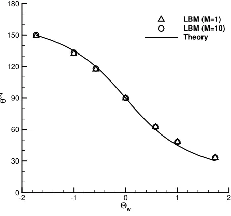
[image:14.612.183.410.230.442.2]LBM (M=1) LBM (M=10) Theory
Figure 3: Contact angle as a function of Θw for the viscosity ratios M = 1 (represented
to simulate fluid-surface interactions and identified that the BGK model produces incorrect results for the equilibrium contact angle due to strong spurious velocities when the binary fluids have different viscosities. To ex-amine whether this also happens to the present model, two different viscosity ratios (M = νR
νB) are investigated: (a) M = 1 with νR = νB = 0.2, and (b) M = 10 with νR = 0.35 and νB = 0.035. The other parameters are fixed as ρR = ρB = 1 and σ = 0.02. Each simulation is run until the shape of droplet does not change, i.e., reaching an equilibrium state. Different contact angles can be achieved through adjusting the dimensionless parameter Θw according to Eq. (26). Fig. 2 shows equilibrium shapes of the droplet with Θw = √3, 0 and −√3 for the viscosity ratio M = 10. Their corresponding equilibrium contact angles, calculated from the measured droplet height and base diameter, are 33.1◦, 89.7◦ and 149.2◦, respectively. The simulated
equi-librium contact angle as a function of Θw forM = 1 andM = 10 is presented in Fig. 3. It is clearly observed that the simulation results are independent of the viscosity ratio, and are in good agreement with the theoretical solution, Eq. (27), in the range of contact angles from 30◦ to 150◦. A numerical
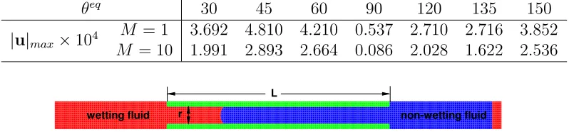
artifact observed in many numerical methods is the presence of spurious velocities at the phase interface. This is also true in our case. Table 1 shows the maximum spurious velocities (|u|max) at
various θeq for M = 1 and 10, where the values of
|u|max are
mag-nified by 104 times. For all of the cases considered, the maximum spurious velocities are of orderO(10−4)or even smaller, comparable to those produced by a recently improved color-fluid model in the stationary bubble test [31], where the bubble is immersed in an infinite domain. Several techniques have been proposed to reduce unwanted spurious velocities in multiphase LB models, and they include increasing the isotropy order of the interfacial force [57], improving the force scheme [58, 59, 60], and using the multiple-relaxation-time (MRT) model instead of the BGK model [61, 59, 9]. Discussion of their usefulness in the present model is beyond the scope of this paper.
Table 1: The maximum spurious velocities (|u|max) at variousθeq forM= 1 and
10. All angles are shown in degrees.
θeq 30 45 60 90 120 135 150
|u|max×104 M = 1 3.692 4.810 4.210 0.537 2.710 2.716 3.852
M = 10 1.991 2.893 2.664 0.086 2.028 1.622 2.536
wetting fluid non-wetting fluid
L r
Figure 4: (Color online) Simulation setup for capillary intrusion. The intruding (red) fluid is the wetting phase while the defending (blue) fluid is the non-wetting phase. The portion in the center of the domain is a capillary tube of lengthL.
the gravity and inertial effects are neglected, this balance can be expressed as [63, 64]
σcos(θ) = 6
r [ηRx+ηB(L−x)] dx
dt, (41)
where θ is the contact angle, r is the capillary tube width, x is the posi-tion of the phase interface, and ηR and ηB are the dynamic viscosities of the red (wetting) and blue (non-wetting) fluids, respectively. In the analytical derivation, θ is specified as a wall boundary condition. However, for com-parison with simulations or experiments, θ should be taken as the dynamic contact angle [63, 64]. The system consists of a 400×25 lattice domain with periodic boundary conditions used in the x direction. In the middle portion the boundaries of the capillary tube are no-slip and wetting. The length of the capillary tube is taken as L = 200 lattices. Outside of the middle por-tion, the boundary conditions are periodic in the y direction. We run the simulations with the parameters ρR =ρB = 1, σ = 5×10⁻³ and r = 15 for two different viscosity ratios: (a) M = 1 and (b) M = 10. The equilibrium contact angle is chosen as θeq = 45◦ to represent hydrophilic capillary tube
for the intruding red fluid. Fig. 5 shows the comparison between our sim-ulation results and the analytical predictions from Eq. (41) for M = 1 and 10. Note that Eq. (41) is plotted using the dynamic contact angle, measured from our LB simulations. For M = 1 and M = 10, the measured dynamic contact angles are respectively θ = 52.23◦ and 52.69◦, which are very close
t
x(
t)
0 200000 400000 600000 800000
0 50 100 150 200
t
x(
t)
0 200000 400000 600000 800000
0 50 100 150 200
Figure 5: (Color online) The length of the column of the intruding fluid,x(t), as a function of time for the viscosity ratios of (a) M = 1 and (b) M = 10. The (red) open circles represent simulation results and the (blue) solid lines are the theoretical predictions from Eq. (41).
Lx
T=TH-Gx T=TL
∂nT=0 ∂nT=0
R x
[image:17.612.127.468.86.224.2]y Ly
Figure 6: Schematic diagram of a liquid droplet on a solid substrate subject to a uniform temperature gradient. The upper wall is set to be a constant temperature TL and the
adiabatic boundary conditions are imposed for the sidewalls. A semi-circular droplet is initially placed on the bottom substrate with its center located at (Lx/2,0).
3.2. Thermocapillary migration of a microdroplet on a horizontal solid sub-strate
In this section, the developed color-fluid LB model is applied to numeri-cally study thermocapillary migration of a liquid droplet on a horizontal solid surface subject to a uniform temperature gradient.
At first, we give a brief description of the problem setup. As shown in Fig. 6, a stationary semicircular droplet of radius R = 50 is initially placed on a smooth substrate at the bottom. The computational domain size is
Lx ×Ly = 16R ×3R and the initial droplet center is (x0, y0) = (8R,0).
[image:17.612.150.462.298.369.2]and T = TL at x= Lx. A constant temperature T =TL is specified on the top wall and the adiabatic boundary conditions are applied for the sidewalls, i.e., ∂nT = 0. We follow the method of Liu et al. [65] to implement these temperature boundary conditions. To account for the effect of temperature on interfacial tension, Eq. (11) is used withσT =−4×10⁻⁴,σref = 4.5×10⁻², and Tref = TL = 0. Besides, we choose TH = 80 so that the horizontal temperature gradient G= 0.1 on the bottom wall.
The thermocapillary migration can be characterized by several important dimensionless parameters: Reynolds number (Re), Marangoni number (M a), capillary number (Ca), and the ratios of viscosity (M) and thermal conduc-tivity (χ) of fluids. By choosing the blue fluid as the continuous phase, these dimensionless parameters are defined as
Re= RU
νB
, M a= RU
κB
, Ca= U ρνB
σref
, χ = κR
κB
, (42)
whereU =−σTGR
ρνB is the characteristic velocity of the system. Note that the
viscosity ratio M has been defined in Subsection 3.1. In addition, the sur-face wettability plays an important role in determining the thermocapillary migration process in a microchannel due to large surface-to-volume ratio, which is described by the equilibrium contact angle θeq. In this study, the influence of surface wettability and M on droplet dynamic behavior will be investigated for constant Re, Ca, M a and χ, unless otherwise stated,
which are fixed at 10, 4.4×10⁻², 10, and 1, respectively.
The influence of contact angle is first investigated for a fixed viscosity ratio, i.e., M = 1. Five different contact angles are used in the simulations, i.e., θeq= 30◦, 60◦, 90◦, 120◦ and 150◦, which are achieved through adjusting
the value of Θw whilst keeping the other parameters fixed. For all contact angles under consideration, the self-motion of the droplet is driven by the thermo-induced interfacial tension gradient on the substrate. However, the droplet motion can undergo two different states, depending on the value of θeq: the droplet migrates from the region of high temperature to the colder region on hydrophilic surfaces, i.e., θeq = 30◦ and 60◦; and the droplet
migrates from the region of low temperature to the warmer region on neutral and hydrophobic surfaces, i.e., θeq ≥90◦. The two states can be observed in
Fig. 7 (since the droplet position has changed from its initial value (x0, y0)),
which plots the flowfield (including the velocity vectors and streamlines) and the corresponding temperature field surrounding the moving droplet for various θeq at t = 2
Y
250 300 350 400 450 20 40 60 80 100 120 Y
350 400 450 500 550 20 40 60 80 100 120 Y
200 250 300 350 400 20 40 60 80 100 120 40 35 30 25 20 15 10 5
350 400 450 500 550 20 40 60 80 100 120 5045 40 35 30 25 20 15 10 Y
250 300 350 400 450 20 40 60 80 100 120 6055 5045 40 35 30 25 20 15 Y
150 200 250 300 350 20 40 60 80 100 120 Y
150 200 250 300 350 20 40 60 80 100 120 Y
450 500 550 600 650 700 20 40 60 80 100 120 (a) (b) (c) (d) (e) 30 25 20 15 10 5 X Y
450 500 550 600 650 700 20 40 60 80 100 120 5550 45 40 35 30 25 20 15 10 Y
200 250 300 350 400 20 40 60 80 100 120
Figure 7: (Color online) The flow field (the left plane) and the temperature field (the right plane) surrounding the moving droplet forM = 1 at the contact angle: (a) 30◦, (b) 60◦,
(c) 90◦, (d) 120◦and (e) 150◦. The red lines are zero contours of ρN, the blue lines with
[image:19.612.147.464.131.510.2]force balance between the shear stresses exerted by the solid surface on the droplet and the pressure difference from thermally induced interfacial tension gradient, which is given by [66]
(σAcosθA−σRcosθR) +sw = 0, (43) wheresw is the integration of shear stresses along the droplet/solid interface, and the subscripts A and R refer to the advancing and receding sides of the moving droplet. Since the shear force prevents the relative motion of the droplet, we have sw < 0, which leads to σAcosθA > σRcosθR. We further assume that the contact angle hysteresis is small, i.e., θA≈θR, which will be demonstrated below. Thus, for hydrophilic surfaces we can obtain σA> σR, implying that the droplet moves towards the region with low temperature. Conversely, the droplet moves towards the region with high temperature for hydrophobic surfaces because σA< σR.
As shown in the left column of Fig. 7, the vortices can be clearly seen surrounding the droplet for all θeq but exhibit different features. For the lowest contact angle, i.e., θeq = 30◦ a small vortex with clockwise rotation
is observed at the bottom wall near the left meniscus inside the droplet. Meanwhile, an external vortex appears on the top of the droplet. When
θeq increases to 60◦, the internal vortex grows which can almost occupy the
left-half space inside the droplet. We also notice that the flows are relatively weak and no backward flows occurs in the region adjacent to the front end of the droplet. For θeq
≥90◦, two pairs of vortices are clearly visible inside and
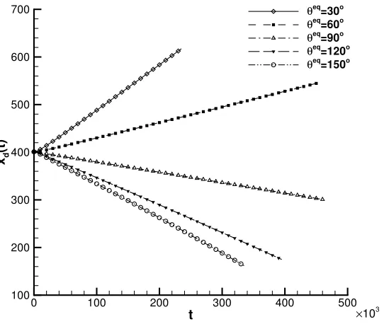
t
xd
(t
)
0 100 200 300 400 500
100 200 300 400 500 600
700 θeq=30o
θeq=60o
θeq=90o
θeq=120o
θeq=150o
[image:21.612.173.444.73.302.2]×103
Figure 8: Time evolution of the x-coordinate of droplet centroid for M = 1 at various contact angles.
interface due to a low curvature, and thus one cannot see the second internal vortex formed near the right meniscus. For neutral and hydrophobic surfaces, the high interface curvature causes different temperature gradients at the left and right segments of the droplet interface, inducing a pair of counter-rotating vortices inside the droplet: the left vortex is bigger in size and stronger in intensity due to higher temperature gradient along the droplet interface.
In order to quantify the effect of surface wettability on droplet motion, Fig. 8 plots the time evolution of the x-coordinate of droplet centroid for
M = 1 at various θeq, calculated by
xd(t) =
R
V ρ NxdV
R
V ρ
NdV =
P
xx(x, t)ρ
N(x, t)
P
xρ
N(x, t) , whereρ N
>0. (44)
Obviously, xd varies linearly with the time for each θeq, suggesting that the droplet migrates on the substrate at a constant velocity. For θeq < 90◦
the droplet migrates in the positive x-direction (i.e., from the hot to cold ends), whereas forθeq≥90◦ it moves reversely. This result is consistent with
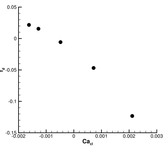
Cacl
fd
-0.002 -0.001 0 0.001 0.002 0.003
[image:22.612.172.446.68.310.2]-0.15 -0.1 -0.05 0 0.05
Figure 9: Dimensionless driving force fd acting on the moving droplet versus the contact-line capillary number Cacl at variousθeq forM = 1.
direction of droplet migration is opposite for the contact angles smaller and larger than 90◦. By differentiating x
d with respect to time, we obtain that, the migration velocities are 9.5×10⁻⁴, 3.22×10⁻⁴,−2.17×10⁻⁴,−5.76×10⁻⁴
and −7.3×10⁻⁴ for θeq = 30◦, 60◦, 90◦, 120◦ and 150◦, respectively. This
[image:22.612.173.443.523.586.2]indicates that more hydrophilicity or hydrophobicity favors to enhance the magnitude of migration velocity. It is therefore not surprising that the droplet can climb up an inclined superhydrophilic substrate as a result of thermally induced Marangoni stresses, against the action of gravity [18].
Table 2: Dynamic contact angles and contact angle hysteresis of a liquid droplet at various θeq forM= 1. All angles are shown in degrees.
θeq 30 60 90 120 150
θA 36.33 64.43 89.64 115.19 144.34
θR 34.34 63.95 89.14 113.66 142.01 (θA−θR) 1.99 0.47 0.49 1.34 2.33
the dynamic contact angles is evaluated as the intersection angle between the droplet interface tangent and the solid surface. The tangent is calculated by the connecting line of two intersection points, which are produced by the interface with the solid surface (denoted as point A) and the interface with the adjacent grid layer (denoted as point B), respectively. Although a constant contact angle (equal toθeq) is imposed through Eq. (26) at the solid surface,
the measured dynamic contact angle is different from θeq because
the contact line motion can cause the relative position of point B (with respect to point A) to change, deviating from the one in static state. It is observed that the advancing and receding contact angles are both greater than θeq for a hydrophilic surface, but smaller than θeq for a hydrophobic or neutral surface. We can also see that the difference between the dynamic contact angles and θeq is negligibly small for a neutral surface, suggesting that the capillary flow is not induced inside the droplet. Thus, the thermocapillary flow dominates the droplet dynamic behavior in this case. In addition, θA is found to be greater than θR for all contact angles considered. However, the contact angle hysteresis is insignificant— typically in the range of (θA− θR) ≤ 2.33◦, which is consistent with the previous experimental and numerical findings [12, 67]. Further, Fig. 9 shows the variation of the dimensionless driving force (fd) with
the contact-line capillary number (Cacl) in the steady state. The
dimensionless driving force is defined as fd = σlcosθσl−σrcosθr
ref , where
the subscripts ‘l’ and ‘r’ denote the three-phase contact points on the left and right, respectively. The contact-line capillary number is defined as Cacl = uσclρνB
ref , where ucl is the contact-line velocity.
We can observe that fd decreases monotonously with an increase
in Cacl. However, |fd| increases with |Cacl| on either hydrophilic
(Cacl >0) or hydrophobic (Cacl <0) surface.
Y
350 400 450 500 550 600 650 700 20
40 60 80 100 120 140
Y
200 250 300 350 400 450 500 550 20
40 60 80 100 120 140
Y
100 150 200 250 300 350 400 450 20
40 60 80 100 120 140
Y
200 250 300 350 400 450 500 550 20
40 60 80 100 120 140
Y
100 150 200 250 300 350 400 450 20
40 60 80 100 120 140
Y
350 400 450 500 550 600 650 700 20
40 60 80 100 120 140
(a) M=0.35 (b) M=3.5
θeq
=30o
θeq
=90o
θeq=150o
Figure 10: (Color online) Droplet shape, position and velocity field surrounding the moving droplet for (a)M= 0.35 and (b)M= 3.5 at the contact angles of 30◦, 90◦and 150◦. The
red lines are zero contours of ρN, and the blue lines with arrows are the velocity vectors.
[image:24.612.124.485.211.424.2]shape and position of the droplet and its surrounding velocity field for the viscosity ratios of 0.35 and 3.5 at t = 1.5×10⁵. For a fixed θeq, one cannot see any significant change in droplet shape withM, and the structure of vor-tices (i.e., velocity field) exhibits similar characteristics to the case ofM = 1 as shown in Fig. 7. However, it is observed that the vortices significantly weaken with an increase in M. For all of the viscosity ratios under consid-eration, the droplet moves toward cooler regions on the hydrophilic surface, i.e., θeq = 30◦, and toward warmer regions on the hydrophobic surface, i.e., θeq = 150◦. On the neutral surface, the direction of droplet motion exhibits
dependence on the value ofM: the droplet moves toward the warmer regions for low M (M ≤1), whereas it moves toward the cooler regions for high M
(M = 3.5). When the asymmetric vortex pair is formed inside the droplet, one can observe a stagnation point (indicated by the pink filled circles in Fig. 10) at the droplet interface, near the midplane of the droplet and closer to the cool end. At the stagnation point, the velocity is zero and the tem-perature is lowest compared to other positions at the interface. To capture the variation of stagnation point with M for a moving droplet, we define a dimensionless position as Xs = xxr−r−xxs
l, where the subscript ‘s’ refers
to the stagnation point. As M is varied from 0.35 to 3.5, we find that
XS decreases from 0.3 to 0.285 and from 0.244 to 0.199 for θeq = 90◦ and 150◦, respectively. This indicates that increasing (decreasing) the migration
[image:25.612.123.486.451.527.2]velocity directed to the cooler (warmer) end leads to the stagnation point shifting from near the midplane to the cooler end.
Table 3: Dynamic contact angles and contact angle hysteresis of a liquid droplet at M= 0.35 and 3.5 for θeq = 30◦, 90◦ and 150◦. All angles are shown in degrees.
M = 0.35 M = 3.5
θeq θ
A θR (θA−θR) θA θR (θA−θR) 30 36.46 34.29 2.16 35.91 34.68 1.23 90 89.93 88.58 1.36 89.52 89.45 0.06 150 144.38 141.26 3.12 144.08 142.87 1.21
Fig. 11 illustrates the time evolution of the x-coordinate of droplet cen-troid for the viscosity ratios of 0.35, 1, and 3.5 at θeq = 30◦, 90◦ and 150◦.
t
xd
(t
)
0 100 200 300 400 500 600
0 100 200 300 400 500 600
700 M=0.35, θeq=30o
M=0.35, θeq=90o
M=0.35, θeq=150o
M=1, θeq=30o
M=1, θeq=90o
M=1, θeq=150o
M=3.5, θeq=30o
M=3.5, θeq=90o
M=3.5, θeq=150o
×103
[image:26.612.181.429.224.441.2]al. [1] that quantifies the thermocapillary migration of a droplet/bubble in an infinite domain. Additionally, it is interesting to find that the viscosity ratio can also change the direction of droplet migration for θeq = 90◦. Although a
high viscosity ratio causes the droplet to migrate toward the cooler regions on the neutral surface, the migration velocity is extremely low (e.g., the case ofM = 3.5 andθeq = 90◦ in Fig. 11). In a viewpoint of practical application,
it is useless to use the thermocapillary flows for controlling a more viscous droplet on a neutral surface since the migration velocity is too weak to coun-teract effectively the external flows. For each fixed M, the droplet generally migrates faster on the hydrophilic surface (i.e., θeq = 30◦) than on the
hy-drophobic surface (i.e., θeq = 150◦). Finally, we find that the viscosity ratio
and the contact angle can also affect the dynamic contact angles and contact angle hysteresis, which is shown in Table 3. For all cases, the advancing and receding contact angles both deviate from the equilibrium contact angle. Specifically, θA and θR are both smaller than θeq for θeq = 90◦ and 150◦ but greater than θeq for θeq = 30◦. Also, θ
A is always larger than θR, resulting in a positive contact angle hysteresis. For a fixed θeq, it can be observed in Table 3 that increasing M can lead to an increase in θR and a decrease in
θA. For each fixed M, the contact angle hysteresis first decreases and then increases as θeq increases, and the lowest hysteresis occurs at θeq = 90◦.
To further investigate the capability of the present model in sim-ulating two-phase fluids with large viscosity differences, i.e., high or low viscosity ratios, we simulate the thermocapillary migration of a droplet on a horizontal solid surface subject to a uniform temper-ature gradient at θeq = 150◦ for M = 1
100, 1
500, and 1
1000. The viscosity of blue fluid is kept at 0.3, and the viscosity of red fluid is varied to obtain different M. The size of computational domain, and the initial location and radius of droplet are kept the same as the above simulations. Re, Ca, M a, and χ are fixed at 0.333,1.33×10−2,1, and
1, respectively. We find that the numerical simulations are still stable for M = 1
100 and
1
x
y
250 300 350 400 450
20 40 60 (b)
x
y
250 300 350 400 450
[image:28.612.169.440.75.278.2]20 40 60 (a)
Figure 12: (Color online) Droplet shape, position and velocity field surrounding the moving droplet for (a) M = 1
100 and (b) M = 1
500 at the contact angle of 150◦. The red lines are zero contours of ρN, and the blue lines with arrows are the velocity vectors.
be caused by low νR, whose value is as low as 3×10⁻⁴.
4. Conclusions
A lattice Boltzmann color-fluid model has been developed to simulate immiscible thermocapillary flows with the presence of fluid-surface interac-tions. Following our previous work [40], the CSF concept is employed to model the interfacial tension forces and the Marangoni stresses because of the gradient of interfacial tension, and the recoloring algorithm proposed by LatvaKokko and Rothman [44] is used to maintain the fluid-fluid interface and overcome the lattice pinning problem. At the solid surface, our recently developed wetting boundary condition [46] is introduced to account for fluid-surface interactions, which can ensure mass conservation for each fluid and suppress spurious velocities at the contact line. An additional convection-diffusion equation is also solved using the passive scalar approach to obtain temperature field, which is related to the interfacial tension by an equation of state.
then used to simulate the transient thermocapillary migration of a microflu-idic droplet on a horizontal solid surface subject to a uniform temperature gradient. Depending on the surface wettability, we numerically demonstrate for the first time that the droplet migration can undergo two different states, i.e., the droplet migrates toward the cooler regions on the hydrophilic surface and toward the warmer regions on the hydrophobic surface, which is consis-tent with the theoretical analysis and experimental observations [66, 15]. For the droplet migration on hydrophilic surfaces, only one vortex is formed in-side the droplet near the rear meniscus; whereas for the droplet migration on neutral and hydrophobic surfaces, two counter-rotating thermocapillary vortices are observed inside the droplet with the one on the warm side always greater in size. Increasing the viscosity ratio of droplet to carrier fluid leads to a reduction in migration velocity due to weakening of thermocapillary con-vection. The viscosity ratio can also affect the direction of droplet migration on the neutral surface, e.g., the droplet migrates toward the warmer regions for M ≤1 but toward the cooler regions forM = 3.5. When the droplet mi-grates on the solid surface, the advancing contact angle is always larger than the receding contact angle, no matter what the viscosity ratio and contact angle, leading a positive contact angle hysteresis. For each fixed M, the con-tact angle hysteresis and the magnitude of migration velocity first decreases and then increases with an increase in θeq, and their minimum values both occur at θeq= 90◦.
Acknowledgments
YHZ thanks the UK’s Royal Academy of Engineering (RAE) and the Leverhulme Trust for the award of a RAE/Leverhulme Trust Senior Research Fellowship.
References
[1] N. Young, J. Goldstein, M. Block, The motion of bubbles in a vertical temperature gradient, J. Fluid Mech. 6 (1959) 350–356.
[2] R. S. Subramanian, R. Balasubramaniam, The Motion of Bubbles and Drops in Reduced Gravity, Cambridge: Cambridge University Press, 2001.
a planar channel by periodic thermocapillary actuation, J. Micromech. Microeng. 18 (2008) 045027.
[4] M.-C. Liu, J.-G. Wu, M.-F. Tsai, W.-S. Yu, P.-C. Lin, I.-C. Chiu, H.-A. Chin, I.-C. Cheng, Y.-C. Tung, J.-Z. Chen, Two dimensional thermo-electric platforms for thermocapillary droplet actuation, RSC Adv. 2 (2012) 1639–1642.
[5] C. Baroud, J.-P. Delville, F. Gallaire, R. Wunenburger, Thermocapillary valve for droplet production and sorting, Phys. Rev. E 75 (2007) 046302. [6] M. L. Cordero, D. R. Burnham, C. N. Baroud, D. McGloin, Thermo-capillary manipulation of droplets using holographic beam shaping: mi-crofluidic pin ball, Appl. Phys. Lett. 93 (2008) 034107.
[7] C. Baroud, M. Robert de Saint Vincent, J.-P. Delville, An optical tool-box for total control of droplet microfluidics, Lab Chip 7 (2007) 1029– 1033.
[8] M. Robert de Saint Vincent, R. Wunenburger, J.-P. Delville, Laser switching and sorting for high speed digital microfluidics, Appl. Phys. Lett. 92 (2008) 154105.
[9] H. Liu, A. J. Valocchia, Y. Zhang, Q. Kang, Lattice Boltzmann phase-field modeling of thermocapillary flows in a confined microchannel, J. Comput. Phys. 256 (2014) 334–356.
[10] V. Pratap, N. Moumen, R. S. Subramanian, Thermocapillary motion of a liquid drop on a horizontal solid surface, Langmuir 24 (2008) 5185– 5193.
[11] J. B. Brzoska, F. Brochard-Wyart, F. Rondelez, Motions of droplets on hydrophobic model surfaces induced by thermal gradients, Langmuir 9 (1993) 2220–2224.
[12] J. Z. Chen, S. M. Troian, A. A. Darhuber, S. Wagner, Effect of contact angle hysteresis on thermocapillary droplet actuation, J. Appl. Phys. 97 (2005) 014906.
[14] Y.-T. Tseng, F.-G. Tseng, Y.-F. Chen, C.-C. Chieng, Fundamental stud-ies on micro-droplet movement by Marangoni and capillary effects, Sen-sors and Actuators A: Physical 114 (2004) 292 – 301.
[15] C. Song, K. Kim, K. Lee, H. K. Pak, Thermochemical control of oil droplet motion on a solid substrate, Applied Physics Letters 93 (8) (2008) 084102.
[16] M. L. Ford, A. Nadim, Thermocapillary migration of an attached drop on a solid surface, Phys. Fluids 6 (9) (1994) 3183–3185.
[17] M. K. Smith, Thermocapillary migration of a two-dimensional liquid droplet on a solid surface, J. Fluid Mech. 294 (1995) 209–230.
[18] G. Karapetsas, K. C. Sahu, O. K. Matar, Effect of contact line dynam-ics on the thermocapillary motion of a droplet on an inclined plate, Langmuir 29 (2013) 8892–8906.
[19] J. H. Snoeijer, B. Andreotti, Moving contact lines: Scales, regimes, and dynamical transitions, Annu. Rev. Fluid Mech. 45 (2013) 269–292. [20] C. Hirt, B. Nichols, Volume of fluid (VOF) method for the dynamics of
free boundaries, J. Comput. Phys. 39 (1981) 201–225.
[21] D. Gueyffier, J. Li, A. Nadim, R. Scardovelli, S. Zaleski, Volume-of-fluid interface tracking with smoothed surface stress methods for three-dimensional flows, J. Comput. Phys. 152 (2) (1999) 423–456.
[22] M. Sussman, E. Fatemi, P. Smereka, S. Osher, An improved level set method for incompressible two-phase flows, Comput. Fluids 27 (1998) 663–680.
[23] S. Osher, R. P. Fedkiw, Level sets methods and dynamic implicit sur-faces, Springer, 2003.
[24] W. Shyy, R. W. Smith, H. S. Udaykumar, M. M. Rao, Computational fluid dynamics with moving boundaries, Taylor & Francis, Washington, DC, 1996.
[26] H.-Y. Chen, D. Jasnow, J. Vi˜nals, Interface and contact line motion in a two phase fluid under shear flow, Phys. Rev. Lett. 85 (2000) 1686–1689. [27] S. Chen, G. D. Doolen, Lattice Boltzmann method for fluid flows, Annu.
Rev. Fluid Mech. 30 (1) (1998) 329–364.
[28] A. K. Gunstensen, D. H. Rothman, S. Zaleski, G. Zanetti, Lattice Boltz-mann model of immiscible fluids, Phys. Rev. A 43 (8) (1991) 4320–4327. [29] I. Halliday, R. Law, C. M. Care, A. Hollis, Improved simulation of drop dynamics in a shear flow at low Reynolds and capillary number, Phys. Rev. E 73 (5) (2006) 056708.
[30] T. Reis, T. N. Phillips, Lattice Boltzmann model for simulating immisci-ble two-phase flows, Journal of Physics A: Mathematical and Theoretical 40 (14) (2007) 4033–4053.
[31] H. Liu, A. J. Valocchi, Q. Kang, Three-dimensional lattice Boltzmann model for immiscible two-phase flow simulations, Phys. Rev. E 85 (2012) 046309.
[32] M. R. Swift, E. Orlandini, W. R. Osborn, J. M. Yeomans, Lattice Boltz-mann simulations of liquid-gas and binary fluid systems, Phys. Rev. E 54 (5) (1996) 5041–5052.
[33] H. Zheng, C. Shu, Y. Chew, A lattice Boltzmann model for multiphase flows with large density ratio, J. Comput. Phys. 218 (1) (2006) 353–371. [34] T. Lee, L. Liu, Lattice Boltzmann simulations of micron-scale drop
im-pact on dry surfaces, J. Comput. Phys. 229 (20) (2010) 8045–8063. [35] X. Shan, H. Chen, Lattice Boltzmann model for simulating flows with
multiple phases and components, Phys. Rev. E 47 (3) (1993) 1815–1819. [36] X. Shan, H. Chen, Simulation of nonideal gases and liquid-gas phase transitions by the lattice Boltzmann equation, Phys. Rev. E 49 (1994) 2941–2948.
[38] X. He, S. Chen, R. Zhang, A lattice Boltzmann scheme for incompress-ible multiphase flow and its application in simulation of Rayleigh-Taylor instability, J. Comput. Phys. 152 (2) (1999) 642–663.
[39] J. Zhang, Lattice Boltzmann method for microfluidics: models and ap-plications, Microfluid. Nanofluid. 10 (1) (2011) 1–28.
[40] H. Liu, Y. Zhang, A. J. Valocchi, Modeling and simulation of thermocap-illary flows using lattice Boltzmann method, J. Comput. Phys. 231 (12) (2012) 4433–4453.
[41] H. Liu, A. J. Valocchi, Y. Zhang, Q. Kang, A phase-field-based lattice-Boltzmann finite-difference model for simulating thermocapillary flows, Phys. Rev. E 87 (2013) 013010.
[42] S. V. Lishchuk, C. M. Care, I. Halliday, Lattice Boltzmann algorithm for surface tension with greatly reduced microcurrents, Phys. Rev. E 67 (2003) 036701.
[43] J. U. Brackbill, D. B. Kothe, C. Zemach, A continuum method for mod-eling surface tension, Journal of Computational Physics 100 (2) (1992) 335–354.
[44] M. Latva-Kokko, D. H. Rothman, Diffusion properties of gradient-based lattice Boltzmann models of immiscible fluids, Phys. Rev. E 71 (2005) 056702.
[45] Y. Peng, C. Shu, Y. Chew, Simplified thermal lattice Boltzmann model for incompressible thermal flows, Phys. Rev. E 68 (2003) 026701. [46] Y. Ba, H. Liu, J. Sun, R. Zheng, Color-gradient lattice Boltzmann model
for simulating droplet motion with contact-angle hysteresis, Phys. Rev. E 88 88 (2013) 043306.
[47] H. Ding, P. D. M. Spelt, Wetting condition in diffuse interface simula-tions of contact line motion, Phys. Rev. E 75 (2007) 046708.
[49] Y. H. Qian, D. D’Humi`eres, P. Lallemand, Lattice BGK models for Navier-Stokes equation, Europhys. Lett. 17 (1992) 479–484.
[50] Z. Guo, C. Zheng, B. Shi, Discrete lattice effects on the forcing term in the lattice Boltzmann method, Phys. Rev. E 65 (2002) 046308.
[51] Y. Q. Zu, S. He, Phase-field-based lattice Boltzmann model for incom-pressible binary fluid systems with density and viscosity contrasts, Phys. Rev. E 87 (2013) 043301.
[52] S. Leclaire, M. Reggio, J.-Y. Tr´epanier, Numerical evaluation of two recoloring operators for an immiscible two-phase flow lattice Boltzmann model, Applied Mathematical Modelling 36 (2012) 2237–2252.
[53] I. Halliday, A. P. Hollis, C. M. Care, Lattice Boltzmann algorithm for continuum multicomponent flow, Phys. Rev. E 76 (2007) 026708. [54] H. Liu, Y. Zhang, Droplet formation in microfluidic cross-junctions,
Phys. Fluids 23 (8) (2011) 082101.
[55] H. Ding, P. D. M. Spelt, Inertial effects in droplet spreading: a compar-ison between diffuse-interface and level-set simulations, J. Fluid Mech. 576 (2007) 287–296.
[56] C. M. Pooley, K. Furtado, Eliminating spurious velocities in the free-energy lattice Boltzmann method, Phys. Rev. E 77 (2008) 046702. [57] X. Shan, Analysis and reduction of the spurious current in a class of
multiphase lattice Boltzmann models, Phys. Rev. E 73 (2006) 047701. [58] T. Lee, P. F. Fischer, Eliminating parasitic currents in the lattice
boltz-mann equation method for nonideal gases, Phys. Rev. E 74 (4) (2006) 046709.
[61] C. M. Pooley, H. Kusumaatmaja, J. M. Yeomans, Contact line dynamics in binary lattice Boltzmann simulations, Phys. Rev. E 78 (5) (2008) 056709.
[62] E. W. Washburn, The dynamics of capillary flow, Phys. Rev. 17 (1921) 273–283.
[63] F. Diotallevi, L. Biferale, S. Chibbaro, A. Lamura, G. Pontrelli, M. Sbra-gaglia, S. Succi, F. Toschi, Capillary filling using lattice Boltzmann equa-tions: The case of multi-phase flows, Eur. Phys. J. Special Topics 166 (2009) 111–116.
[64] C. Pooley, H. Kusumaatmaja, J. Yeomans, Modelling capillary filling dynamics using lattice Boltzmann simulations, Eur. Phys. J. Special Topics 171 (1) (2009) 63–71.
[65] C.-H. Liu, K.-H. Lin, H.-C. Mai, C.-A. Lin, Thermal boundary condi-tions for thermal lattice Boltzmann simulacondi-tions, Comput. Math. Appl. 59 (2010) 2178–2193.