S
TRATHCLYDE
D
ISCUSSION
P
APERS IN
E
CONOMICS
D
EPARTMENT OF
E
CONOMICS
U
NIVERSITY OF
S
TRATHCLYDE
PERSONAL INDEBTEDNESS, SPATIAL EFFECTS AND
CRIME
B
Y
STUART MCINTYRE AND DONALD LACOMBE
Paper presented during the 25th ERSA Summer School at Umeå University, Sweden. July 2012.
Keywords: Spatial Econometrics, Crime, Personal Debt, Economic Conditions
JEL Codes: R1, K42, C11, C21
Personal Indebtedness, Spatial E
ff
ects and Crime
Stuart G. McIntyre
∗Donald J. Lacombe
†May 22, 2012
Abstract
There is a long and detailed history of attempts to understand what causes crime. One of the most prominent strands
of this literature has sought to better understand the relationship between economic conditions and crime. Following
Becker (1968), the economic argument is that in an attempt to maintain consumption in the face of unemployment,
people may resort to sources of illicit income. In a similar manner, we might expect ex–ante, that increases in the
level of personal indebtedness would be likely to provide similar incentives to engage in criminality. In this paper we
seek to understand the spatial pattern of property and theft crimes using a range of socioeconomic variables,
including data on the level of personal indebtedness.
∗
StuartG.McIntyre (corresponding author), DepartmentofEconomics,Universityof Strathclyde, Sir William Duncan Building, 130 Rottenrow, Glasgow G4 0GE, Scotland, UK; Phone: +44 (0)141 548 3858 (Ext. 3858), [email protected]
†
1 Introduction
The recent global recession has brought the issue of the relationship between economic conditions
and crime to the fore of public and scholarly debate. There has been extensive scholarly work
attempting to understand the causes of crime (Kelly 2000, Wilson & Herrnstein 1985, Cohen &
Felson 1979, Kvalseth 1977, Danziger 1976). Particularly interesting has been the study of the
relationship between unemployment and crime (Carmichael & Ward 2001, Pyle & Deadman 1994,
Cantor & Land 1985, Becker 1968). In this paper, we use spatial econometric methods to examine
an aspect of the relationship between economic conditions and crime that, to our knowledge,
has gone unremarked upon to date; namely the relationship between personal indebtedness and
crime. While there are spatial crime regressions in the literature1, for instance Anselin et al.
(2000), Cracolici & Uberti (2009) and Buonanno et al. (2012), little attention is paid to the
insights that can be gained by considering thedirectandindirecteffects2in the context of crime
analysis.
2 Material and methods
Given the geographic nature of crime data (Schmid 1960, Voss & Petersen 1971), it is reasonable
to suspect that spatial autocorrelation may be an issue when modelling crime data. Spatial
autocorrelation can pose problems when using standard econometric techniques, such as OLS
(LeSage & Pace 2009). Therefore we propose using Bayesian spatial econometrics methods in
this paper (see LeSage & Pace (2009) for a textbook outline of these models and methods).
There are three standard spatial econometric models, the spatial autoregressive (SAR) model,
the spatial error (SEM) model, and the spatial Durbin model (SDM). The motivation for each
model is noted below:
• In the SAR model spatial autocorrelation is exhibited in the dependent variable. From an
econometric perspective, if the true data generating process (DGP) for the data is the SAR
model, and one utilizes, for example, OLS for estimation purposes, the resulting coefficient
estimates will be biased and inconsistent due to the endogeneity of the term on the right
hand side of the equation (LeSage & Pace 2009).
1
Although Buonanno et al. (2012, 194-195) argues that these methods are still rarely utilised by those economists studying crime issues.
2
Thedirecteffect, can be considered the ‘within area’ effect. Theindirecteffect can be considered the impact
of a change in the explanatory variable in one area, on the dependent variable in neighbouring areas. Thetotal
• The SEM model posits that the spatial autocorrelation is found in the error term. It is
possible that for a variety of reasons, when an econometric model is specified and estimated,
certain factors that should be included in the model are not and that these factors are
correlated over space, resulting is residual spatial error correlation. If the true DGP is the
SEM model and, again for example, OLS is used in the estimation, the OLS estimators
of the coefficients are unbiased but inefficient and the estimates of the variance of the
estimators are biased (LeSage & Pace 2009).
• The spatial Durbin model extends the SAR model by including spatially weighted
explana-tory variables. LeSage & Pace (2009) suggest that the SDM model should be used when
one believes that there may be omitted variables that follow a spatial process and are
correlated with included independent variables.
Our motivation for using Bayesian spatial econometric techniques, as opposed to the more
familiar maximum likelihood paradigm, is that Bayesian methods allow us to make non-nested
model comparisons in a statistically coherent manner, where model choice proceeds by choosing
the model (i.e SAR, SEM or SDM) with the highest posterior probability. In each case we ran the
Gibbs sampler for 5000 draws with a ‘burn-in’ of 500 draws. Homoskedastic and heteroskedastic
versions of each of the 3 models (SAR v. SEM v. SDM) were considered, and proper, but
relatively uninformative priors were used in all cases.
In this paper we use data for London, UK covering 2004/05 and consider 6 theft crimes:
robbery, theft from the person, burglary in a dwelling, burglary of a dwelling, theft of a motor
vehicle and theft from a motor vehicle. Personal indebtedness is measured using data on the
value of county court judgements (CCJ’s) granted in each neighbourhood. Full variable details
are provided in Table 2. All variables used here were studentized. The Office of National
Statistics (hereafter, ONS) provides statistics at several geographical levels. All data used here
are provided at the super output area level which are fixed geographical areas constructed by
the ONS at two principle levels: middle and lower and we utilise the middle layer here (each of
these areas has a minimum of 5000, and an average of 7,200, people within it).
3 Theory/Calculation
While there has been much written on the crime-unemployment relationship (Carmichael &
Ward 2001, Pyle & Deadman 1994, Cantor & Land 1985, Becker 1968) nothing, to our knowledge,
appears in academic journals about the relationship between personal indebtedness and crime.3
Becker (1968) argued that crime, from an economic perspective, stemmed from the inability
of individuals to satisfy their target level of consumption through legitimate means (a similar
argument was made by Cantor & Land (1985, 317)). The unemployed then, theory suggests,
turn to illicit income streams to meet the shortfall in their consumption needs.
Others in the literature, for instance Box (1995), emphasise the emotional strain of becoming
unemployed, and the feelings of anomie that stem from the lack of legitimite means for
advance-ment. Additional sociological issues such as the ecology of the local area (Voss & Petersen 1971)
and the degree of education (Ehrlich 1975) are also thought to be important determinants of
crime. This line of inquiry maintains that, since everyone who suffers economic hardship does
not resort to criminality, there must be a reason why some people do and others do not.
We suggest that it is possible to view personal debt as providing the initial means of
con-sumption smoothing following economic hardship. Whereas, in the case of the relationship
between crime and unemployment, the view in the literature is almost of a seemless transition
from employment to unemployment and an attraction to criminality. However, there could be
an important intermediate role to be played by personal debt. An individual made unemployed
may seek to access credit as a means of bridging the initial consumption gap, and it is only when
they can access no more credit and have defaulted on their existing loans, that they are driven
to commit crime to access an illicit income stream a l´a Becker (1968).
4 Results & Discussion
The first thing to note is that in all our regression models the spatial autocorrelation coefficient
is significant, indicating that spatial autocorrelation is present in the data for all crime categories
considered, justifying the use of spatial econometric methods. In our spatial regressions analyses,
we used a contiguity weight matrix for each of the three standard spatial econometric models
defined earlier in this paper4. The second thing to note is that, as previous studies have found,
for instance Cantor & Land (1985) and Cherry & List (2002), we find that the explanatory
variables that are important in explaining the observed pattern of crime vary across crime type,
requiring the use of disaggregated crime measures.
3
A number of papers written in the 1970’s in the United States addressed the general impact of economic crises on crime, see Brenner (1971, 1976, 1978), Brenner & Harvey (1978), Cohen & Felson (1979).
4
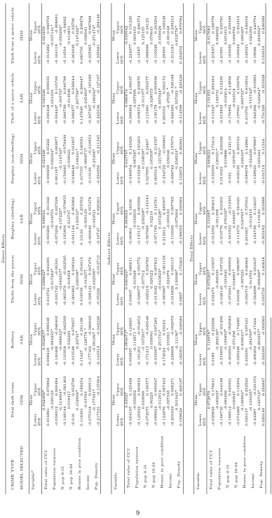
A brief note about Table 1 may be helpful to the reader. For each of the seven categories
of crime5, recall that we only present the results from the spatial econometric model, for each
crime type, which has the highest posterior probability–the model selected for each crime type
is noted in row 2 of Table 1. For each model, following LeSage & Pace (2009), we calculate
the direct, indirect and total effect of each explanatory variable6. The direct effect, can be
considered the ‘within area’ effect. Theindirect effect can be considered the impact of a change
in the explanatory variable in one area, on the dependent variable in neighbouring areas. The
total effect is the sum of the direct and indirect effects.
In motivating this article we made specific reference to both the spatial dimension of this
study, and our focus on the role of personal indebtedness. Taking these in reverse order, we
can see from our results that personal indebtedness has an important role to play in explaining
the observed pattern of personal theft crimes in London, UK. In the case of Robbery, we find
that the level of personal indebtedness in an area is positively related to Robbery in that area
and in surrounding areas. We obtain the same result for ‘thefts from the person’; an offence
which differs from that of Robbery only in the degree of violence used. For the other theft crime
measures considered, the level of personal indebtedness in an area is not found to be associated
with the dependent variable.
Just as the importance of personal indebtedness, noted a moment ago, varies across crime
type, the same is true of other explanatory variables. A good example of this is our finding
that income is directly and negatively associated with thefts of cars, but, is not significantly
associated with theftsfrom cars. A plausible explanation for this is that in areas with higher
incomes, cars have more sophisticated alarm and immobilser systems and are therefore harder
to steal. Stealing from a car meanwhile, is perhaps as easy for a more expensive car as an
inexpensive car.
Just as important as the distinction between different types of crimes and the explanatory
variables that are important in explaining them, is the direct and indirect effects distinction
introduced earlier. To see the insights that this can provide, note the role of income in explaining
the observed pattern of robberies. Income is negatively directly and indirectly associated with
robberies. This means that the lower the income in an area, the more robberies take place in
that area, and in neighbouring areas. This lends direct support to the argument that poverty is
associated with crime, and that poverty induces crime spillovers. The same relationship is found
5
The first crime type is an aggregation of the other 6 categories of theft crime considered here.
6
Our posterior model probability calculations did not support the SEM model for any crime type, and chose the heteroskedastic model in each case.
for the ‘housing in poor condition’ variable for robberies.
In the case of ‘thefts from the person’ however, the relationship with houses in poor condition
is more complex. Here we find that the more houses in poor condition there are in an area, the
more thefts from the person in that area, but the fewer in surrounding areas. We think that
what we are starting to get at with this particular result is some of the richness of explanations
for the observed patterns of crime. In this case, those who venture out of their neighbourhoods
to rob people are perhaps more experienced, older criminals who are more likely to use violence
while robbing people, as compared to younger less mobile, less experienced criminals who seek
to do the same thing in their own area, just with less violence. This is pure conjecture, but
by examining the direct and indirect effects in this way we get a more complete picture of the
complex spatial relationship underpinning observed patterns of crime.
A final aspect of the results that we consider here is the role of houses in poor condition
in explaining the observed pattern of burglary of dwellings and non–dwellings. Houses in poor
condition in an area is directly and positively associated with burglary of dwellings and non–
dwellings in that area. This is not a surprise–the worse condition that houses are in the less
secure they are likely to be, and the less secure that non-dwellings are also likely to be.
5 Conclusions
The main conclusions of this study is that the level of personal indebtedness does matter in
explaining the observed pattern of robberies and thefts from the person. In addition, we have
demonstrated the importance of accounting for spatial autocorrelation in modelling crime data.
Further, we have shown how the calculation of the direct and indirect effects in spatial crime
models can provide important insights into the complex relationship underpinning crime data.
Future work will explore the dynamic nature of these relationships using data for a subsequent
year–the only other year for which personal indebtedness data are available, as well as considering
Bibliography
Anselin, L., Cohen, J., Cook, D., Gorr, W. & Tita, G. (2000), ‘Spatial analyses of crime’,
Criminal Justice4, 213–262.
Becker, G. (1968), ‘Crime and Punishment: An Economic Approach’, The Journal of Political
Economy76(2), 169–217.
Box, S. (1995),Recession, crime and punishment, Macmillan Education, London.
Brenner, H. (1978), Impact of economic indicators on crime indices, in ‘Unemployment and
Crime’, United States Congress.
Brenner, H. & Harvey, M. (1978), ‘Economic crises and crime’,Crimes and societypp. 555–72.
Brenner, M. (1971), Time series analysis of relationships between selected economic and social
indicators, Dept. of Epidemiology and Public Health, Yale School of Medicine.
Brenner, M. (1976), Estimating the social costs of national economic policy: Implications for
mental and physical health, and criminal aggression, Johns Hopkins University, School of
Hygiene and Public Health and Dept. of Social Relations.
Buonanno, P., Pasini, G. & Vanin, P. (2012), ‘Crime and social sanction’, Papers in Regional
Science91(1), 193.
Cantor, D. & Land, K. (1985), ‘Unemployment and crime rates in the post-World War II United
States: A theoretical and empirical analysis’,American Sociological Reviewpp. 317–332.
Carmichael, F. & Ward, R. (2001), ‘Male unemployment and crime in England and Wales’,
Economics Letters73(1), 111–115.
Cherry, T. & List, J. (2002), ‘Aggregation bias in the economic model of crime’, Economics
Letters75(1), 81–86.
Cohen, L. & Felson, M. (1979), ‘On estimating the social costs of national economic policy: a
critical examination of the Brenner study’,Social Indicators Research6(2), 251–259.
Cracolici, M. & Uberti, T. (2009), ‘Geographical distribution of crime in Italian provinces: a
spatial econometric analysis’,Jahrbuch f¨ur Regionalwissenschaft29(1), 1–28.
Danziger, S. (1976), ‘Explaining urban crime rates’,Criminology14(2), 291–296.
Ehrlich, I. (1975), ‘On the relation between education and crime’,NBER Chapterspp. 313–338.
Kelly, M. (2000), ‘Inequality and crime’,Review of Economics and Statistics 82(4), 530–539.
Kvalseth, J. (1977), ‘A note on the effects of population density and unemployment on urban
crime’,Criminology15(1), 105–110.
LeSage, J. P. & Pace, R. K. (2009), Introduction to Spatial Econometrics, CRC Press, Boca
Raton, FL.
LeSage, J. P. & Pace, R. K. (2010), ‘The biggest myth in spatial econometrics’,SSRN.
Pyle, D. & Deadman, D. (1994), ‘Crime and unemployment in Scotland: some further results’,
Scottish Journal of Political Economy41(3), 314–324.
Schmid, C. (1960), ‘Urban crime areas: Part i’,American Sociological Reviewpp. 527–542.
Voss, H. & Petersen, D. (1971),Ecology, crime, and delinquency, Appleton-Century-Crofts.
Wilson, J. & Herrnstein, R. (1985),Crime Human Nature: The Definitive Study of the Causes
Table 2: Variable details
All variables taken fromhttp://www.neighbourhood.statistics.gov.uk/operated by the UK Office of National Statistics (ONS).
Variable Variable description
Value of CCJ Total value of CCJ’s granted in each area in 2004 in (£).
Population turnover Net change in internal migration per 1,000 persons 2004/05.
% pop 0-15 Percentage of population aged 0-15 (mid-2004 model based
esti-mates).
% pop 16-24 Percentage of population aged 16-24 (mid-2004 model based
esti-mates).
Houses in poor condition The modelled probability that a house in the area will fail to meet the UK Government ‘Decent Homes’ standard. Data used are averages of lower super output area values for 2004.
Income Average weekly household total income (ONS model based
esti-mate) 2004/05.
Pop. Density Number of persons usually resident per hectare (based on 2001
census data).