City, University of London Institutional Repository
Citation
:
Wills, A. J. and Pothos, E. M. (2012). On the adequacy of current empirical evaluations of formal models of categorization. Psychological bulletin, 138(1), pp. 102-125. doi: 10.1037/a0025715This is the unspecified version of the paper.
This version of the publication may differ from the final published
version.
Permanent repository link:
http://openaccess.city.ac.uk/1978/Link to published version
:
http://dx.doi.org/10.1037/a0025715Copyright and reuse:
City Research Online aims to make research
outputs of City, University of London available to a wider audience.
Copyright and Moral Rights remain with the author(s) and/or copyright
holders. URLs from City Research Online may be freely distributed and
linked to.
City Research Online: http://openaccess.city.ac.uk/ [email protected]
On the adequacy of current empirical evaluations of formal models of categorization
MS #2010-0444
Revised manuscript for Psychological Bulletin
Abstract
Categorization is one of the fundamental building blocks of cognition, and the study of
categorization is notable for the extent to which formal modeling has been a central and
influential component of research. However, the field has seen a proliferation of divergent,
non-complementary models with little consensus on the relative adequacy of these accounts.
Progress on assessing relative adequacy of formal categorization models against these criteria
has, to date, been limited because (a) formal model comparisons are narrow in the number of
models and phenomena considered, and (b) models do not often clearly define their
explanatory scope. Progress is further hampered by the practice of fitting models with
arbitrarily variable parameters to each data set independently. Reviewing examples of good
practice in the literature, we conclude that model comparisons are most fruitful when relative
adequacy is assessed by comparing well-defined models on the basis of the number and
proportion of irreversible, ordinal, penetrable successes (principles of minimal flexibility,
breadth, good-enough precision, maximal simplicity, and psychological focus).
The study of categorization is a fascinating endeavor. The process of constructing and
using categories underpins our capacity to encode and apply information in the world in an
efficient and competent manner but also, ultimately, our ability to think in terms of abstract
ideas, such as justice, love, and happiness. Categories facilitate communication, and facilitate
inferences about unobserved properties of objects. What are the mechanisms that correspond
to psychological categorization processes? This question has been intensely studied for over
fifty years (e.g. Bruner, Goodnow & Austin, 1956), and has led to some of the most
sophisticated and influential mathematical, computational, and neuroscientific models in
psychology. Indeed, categorization research contains one of the most influential formal
models in all of psychology - the Generalized Context Model (Nosofsky, 1984)1. Yet there is
also a profound divergence among modelers at the most fundamental level. How should
categorization models be compared? What is the ideal form of a categorization model? What
kind of categorization models should we aim to develop? The lack of consensus regarding
such key issues has resulted in categorization research being carried out in increasingly
independent strands and this has been inhibiting overall progress in the field. Nosofsky,
Gluck, Palmeri, McKinley and Glauthier (1994) wrote, “Recent years have seen an avalanche
of newly proposed models of category learning and representation. As such models grow
increasingly more sophisticated, there is a need to develop increasingly more rigorous testing
grounds so that one may choose among them” (p. 352). Almost 20 years later, progress
towards this goal remains limited.
In the current article, we first provide a definition of the term formal model, consider
the principal advantages of formal modeling over other forms of theorizing, briefly
summarize some of the leading formal models of categorization, and assess progress to date
we believe are most likely to lead to progress in the future. We organize our conclusions in
terms of a set of criteria for assessing the relative adequacy of models, and a list of
dependent and independent variables that any adequate formal model of categorization
should be expected to address. Although our focus is on the formal modeling of
categorization, the issues we discuss and the proposals we make are not limited to the field of
categorization research. As we outline below, formal modeling has a number of potential
advantages, and these advantages are quite general. Similarly, the extent to which formal
models deliver those advantages depends on the extent to which the problems and pitfalls
considered in this article are avoided. Categorization research has been chosen for
consideration in this paper because it is one of the parts of psychology in which formal
modeling has featured particularly heavily (of course, not the only area – psycholinguistics
research is another example).
Definition of a formal model
A formal model is one that unambiguously specifies transformations from one or
more independent variables (IVs) to one or more dependent variables (DVs). In the case of
formal models of categorization, one independent variable is category structure and one
dependent variable is categorization accuracy (for an illustration, see Figure 1).
-- Figure 1 about here --
The phrase “unambiguously specifies” is critical for the definition of a formal model.
Byunambiguous specification, we mean that the model must express the nature of the
transformations such that, for a given set of inputs and model parameter values, the model’s
output can be determined with some kind of algorithm. A reasonable proxy for algorithmic
determinability is whether the process of determining the model’s output from its inputs and
Note that unambiguous specification is not the same as determinism; a model’s output might,
for example, be the probability of a particular response. The criterion of unambiguous
specification largely excludes models expressed purely in verbal terms and typically involves
mathematical expression (or expression in terms that can be unambiguously transformed into
algorithmic operations, as in high-level computer programming languages).
The case for formal modeling
As Murphy (2011) points out, formal modeling is not without its disadvantages.
Compared to informal theories, developing formal models is more time consuming and,
perhaps as a result, is arguably more likely to lead to the neglect of empirical phenomena that
lie outside the model’s scope. So why model? There are at least six advantages to a formal
modeling approach – recognition of problem complexity, deeper insight, ambiguity
reduction, model comparison, behavior prediction and the prospect of automated cognition.
We discuss each of these potential advantages of formal models over more informal theories
below:
Recognition of problem complexity
The experience of many modelers is that attempting to transform an informal theory
into a formal model often leads to a recognition that the problem under study is substantially
more complex than was immediately apparent. In categorization research (and in other areas
of psychology) this is partly because informal theories make extensive use of verbal labels
that denote intuitively obvious but computationally complex constructs. For example, in
unsupervised classification (category formation in the absence of feedback), the category
groupings selected most frequently by participants are often those that are most “intuitive” –
but formally specifying what makes them so turns out to be quite complex (Pothos & Bailey,
Deeper insight
In essence, a formal model is a data-reduction technique. Formal models can be
thought of as compressing potentially very large data sets down to a small number of values –
the parameters of the model. The extent to which these parameters allow a reconstruction of
the data through the architecture of the model is the extent to which the compression is
appropriate. As long as the model’s parameters are penetrable, this compression can lead to
insights about empirical data that may not be obvious from the raw data set. We discuss this
advantage further in the “penetrable models” section of the article.
Ambiguity reduction
Definitionally, a formal model is one that unambiguously specifies IV-DV
transformations. As a consequence, the ability of a formal model to encompass a particular
set of empirical findings should be unambiguously determinable, given sufficient information
about the state of the IVs that form part of the model’s input. Of course, to the extent that
there is uncertainty about the empirical phenomenon itself (through, for example,
measurement error) there may be uncertainty about a model’s ability to encompass that
phenomenon.
Behavior prediction and automated cognition
Formal models provide the prospect for prediction of behavior - if we can predict the
output of cognitive processes from their input, we may also be able to reproduce aspects of
cognition in artificial devices. Formal models are able to contribute to behavior prediction
and automated cognition, over and above informal ones, because of the ambiguity reduction
that they entail.
Facilitation of theory comparison
If more than one formal theory exists and, for each of those theories, their ability to
possible to compare the relative adequacy of those models. The potential for unambiguous
determinability in formal models – and the inherent difficulty of unambiguous
determinability in more informal forms of theorizing – constitutes one of the main advantages
of formal modeling.
Divergent, non-complementary models
In this section, we briefly summarize some leading formal models of categorization.
We do this in order to (a) illustrate the divergent, non-complementary nature of current
models, and (b) to provide a context for our proposals concerning the empirical evaluation of
models. The models considered in this section are: the Generalized Context Model, the
Nosofsky-Smith-Minda prototype model, SUSTAIN, COVIS, KRES, the Simplicity model,
and the Rational Model of Categorization. These models were chosen on the basis of either
being highly influential, or encapsulating an important aspect of categorization theory, or
making some unique or original contribution. Even within those criteria, there were a number
of formal models of categorization that were worthy of inclusion, but which we nevertheless
excluded in order to keep this section to a manageable length. Before describing specific
models, we outline at a broad level the components such models typically have, and how
those components relate to each other.
Template for a Formal Model of Categorization
At a general level, the purpose of categorization models is to organize information
from our experience in such a way that it allows, amongst other things, predictions about how
new stimuli should be classified. One can distinguish between the representations upon which
categorization is based and the mechanisms that support the categorization process. However,
such a distinction is not always clear-cut, as the nature of the representations affects the
affects the forms of representation that are plausible. Throughout this paper, the term “formal
model” denotes a specific combination of process and representational assumptions.
-- Figure 2 about here --
Figure 2 shows a broad schema for models of categorization; not all models have all
components. Categorization is seldom modeled from a retinal starting point – most modelers
assume some form of higher-level input representation of the presented stimulus. The
attentionally-modulated information from the input representations activates one or more
intermediate representations (e.g. prototypes, exemplars). Information from the intermediate
representations activates one or more category representations via an evidential mechanism
(e.g. similarity computations). Typically, more than one category representation will be
activated to some degree. Equally, a mechanism has to be in place that can guide the
formation of new categories. Either way, there is a need for a decision mechanism that turns
graded information into a categorical response.
Generalized Context Model
The Generalized Context Model (GCM; Nosofsky, 1984) is the most influential
formal model of categorization to date1. The GCM is a model with exemplar-based
intermediate representations (Figure 2) – in other words, it assumes that categories are
represented through the storage of specific examples of members of those categories. Formal
exemplar models of categorization can be traced back at least as far as Reed’s (1972)
average-distance model, but GCM is most directly related to the Context Model (Medin &
Schaffer, 1978).
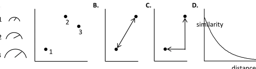
As Figure 3A illustrates, GCM represents stimulus input as points in a
multidimensional space, with inter-item similarity considered to be a decreasing function of
distance in that psychological space. The position of stimuli in that space is sometimes
identification confusion probabilities (Nosofsky, 1986), or pairwise similarity ratings
(Palmeri & Nosofsky, 2001). Distance in psychological space is typically calculated with a
Euclidean metric (Figure 3B) for integral stimuli, but with a city-block metric (Figure 3C) for
separable stimuli. This follows part of Garner’s (1978) operationalization of the
integral-separable distinction (integral stimuli are also, for example, those whose dimensions are
difficult to selectively attend; hue and saturation, for example).
-- Figures 3 and 4 about here --
Following Shepard (1958), the function relating distance in psychological space to
similarity is typically exponential (Figure 3D). This similarity-distance function formalizes
the process assumption that categorical decisions are strongly affected by stimuli that are
close in psychological space, with differences in distance becoming less important as distance
from the presented item increases. Where stimuli are highly confusable, a Gaussian rather
than exponential function is sometimes used; this approximates trial-to-trial variability in
stimulus representation (Ennis, 1988).
GCM also has an attentional mechanism. In GCM, selective attention is considered to
operate on the dimensions of the psychological space (Figure 3A), with attention to
dimension X being represented as a factor by which distances on that dimension are
multiplied in order to calculate similarity. Conceptually, and as illustrated in Figure 4, this
can be considered as the compression and stretching of psychological space. The inclusion of
selective attention in GCM was originally motivated through its ability to provide an account
for certain relationships between identification difficulty and categorization difficulty
(Nosofsky, 1984, 1986). GCM also has a parameter that allows for the overall expansion or
contraction of psychological space (Figure 4C). GCM’s formalization of selective attention
(b) selective attention to stimulus dimensions is a matter of degree, rather than all-or-none,
(c) selective attention occurs at the level of stimulus dimensions.
The output of the GCM is a prediction about the probability with which each of the
available category responses will be produced, as a function of the presented stimulus, and
the nature of the exemplars presented to the participants. GCM’s evidential mechanism
involves the computation of summed similarities. For example, if the available category
responses are A and B, then GCM calculates the sum of the similarities of the presented
stimulus to each of the stored exemplars belonging to category A (SA). The same calculation
is performed for category B (SB). Simplifying slightly (see below), GCM’s decision
mechanism is that the probability of a category A response is
Equation 1
, where γ was a subsequent addition to the model (Ashby & Maddox, 1993; Nosofsky &
Zaki, 2002) in order to allow it to account for the degree of response determinism seen in
participants. As γ becomes large, the probability of selecting the category with the larger
summed similarity approaches 1 and the probability of selecting the category with the smaller
summed similarity approaches 0. Equation 1 is typically expressed in a more general form
that permits more than two response options (Nosofsky, 1984). The calculation of summed
similarities also takes into account memory strength (represented as a multiplicative factor of
the stored item’s similarity score, Nosofsky, 1988) and the decision mechanism can include
category response bias (represented as a multiplicative factor of the summed similarity,
Nosofsky, 1984).
GCM has been the basis of a number of other models. The most influential of these is
connectionist framework, and it provides a formalization of the process by which the
selective attention and memory-strength parameters of GCM change over time. In ALCOVE,
both sets of parameters are determined by gradient descent – an idea closely similar to the
reduction-of-prediction-error accounts of learning and learned attention provided by animal
learning models (Mackintosh, 1975; Rescorla & Wagner, 1972). Other extensions of GCM
include the Extended Generalized Context Model (EGCM, Lamberts, 1995), which
formalizes the assumption that stimulus representations are not perceived instantaneously,
and the Exemplar-Based Random Walk model (Nosofsky & Palmeri, 1997a), which
formalizes the assumption that categorical decision processes are not instantaneous.
In addition to the introduction of a highly influential formal model of categorization,
work on GCM also demonstrated the potential of formal categorization models to provide
very precise quantitative fits to observed phenomena. Indeed, the degree of precision that can
sometimes be achieved by GCM is impressive (e.g. Nosofsky, 1986). The quantitative
examination of a formal model can take a number of different forms and one approach
concerns an emphasis on the minimization of an error term. As we will set out in a later
section, evaluation of formal models solely on the degree to which they can minimize an error
term can be problematic in a number of respects (as researchers working on GCM accept, see
e.g. Nosofsky & Stanton, 2005, p. 613).
The GCM is the most widely known and understood of the current formal models of
categorization. It also one of the most clearly specified. For these reasons alone, many of the
examples employed in the current article are formulated in terms of the GCM. We do not
intend to imply that the GCM is deficient compared to other models. In fact, we believe that
the GCM’s clear specification is a great strength, and one that has facilitated the writing of
Nosofsky-Smith-Minda (NSM) prototype model
Prototype models assume that each category has a single intermediate representation.
That intermediate representation – the category prototype – is typically considered to be the
average of the representations of the category examples, although some models assume that
distributional information is also stored (Fried & Holyoak, 1984). Formal prototype models
of categorization can be traced back at least as far as Reed (1972), but arguably the most
influential version of recent times has been the Nosofsky-Smith-Minda (NSM) prototype
model, originally developed by Nosofsky (1987), and extensively investigated in the work of
Smith and Minda (e.g. Smith & Minda, 1998).
One of the interesting properties of the NSM prototype model is that, except in the
critical aspect of stimulus representation, it is closely similar to the GCM. For example, it
employs the same similarity-distance equations (Figure 3D), and the same decision functions
(Equation 1), as the GCM. Such similarity between models on all but one, theoretically
interesting, issue facilitates model comparison. Work on the NSM model has included
principled attempts to assess the relative adequacy of two qualitatively different formal
models, for example the comparison of NSM with GCM (e.g. Smith, 2002). This is an
approach to model comparison that we advocate throughout this article, as long as the
comparison satisfies certain requirements (we will argue later that certain kinds of
comparisons lead to more compelling conclusions than others). Comparison of qualitatively
different models seems more likely to lead to progress in the field than evaluations of the fit
of a single model or of the relative fit of a number of variants of an a priori favored class of
model. We return to this point in more detail in a later section.
SUSTAIN
SUSTAIN (Love, Medin & Gureckis, 2004) is a formal model of categorization
designed to account for both categorization probabilities and feature-inference probabilities.
It also provides a formal model of the relationship between supervised and unsupervised
category learning (i.e. category learning in the presence and absence of category labels), and
makes different representational assumptions to either the GCM or the NSM prototype
model.
SUSTAIN is able to provide an account of both categorization and feature inference
as a result of being an auto-encoder – in other words, a model that seeks to reproduce and
complete its input at its output. In such models (see also McClelland & Rumelhart, 1985)
categorization and feature inference are differentiated by the nature of the information
missing at input – in categorization, the category label is missing; in category-to-feature
inference, the category label is present at input, but one or more of the features are absent. In
both cases, the model takes this incomplete input, and attempts to reproduce it – with the
missing information “filled in” – at its output.
In common with GCM and NSM, SUSTAIN represents stimulus input within a
psychological space, and allows attentional modulation along the dimensions of that space.
However, the attentional modulation in SUSTAIN affects the narrowness of the receptive
field of cluster representations (see below), rather than GCM’s uniform compression/
expansion of an entire dimension. SUSTAIN also incorporates a bias to focus on a subset of
stimulus dimensions.
In terms of intermediate representations, SUSTAIN is neither an exemplar model, nor
a prototype model. Instead, its representations are clusters. Exemplars and prototypes are
special cases of cluster-based representation and, as is the case with exemplars or prototypes,
there is exactly one cluster for each experimenter-defined stimulus; in prototype-based
representation there is exactly one cluster for each experimenter-defined category.
SUSTAIN forms and develops clusters in a trial-by-trial manner. The first stimulus
presented is assigned its own cluster, centered on that stimulus. In supervised categorization,
subsequent stimuli are assigned to their own cluster if the existing clusters make an incorrect
prediction about the category membership of the presented item. In unsupervised
categorization, a stimulus is assigned a new cluster if it is sufficiently different to the existing
clusters – how different it has to be in order to produce a new cluster is a free parameter (i.e.
a parameter whose value is assumed to be whatever makes the model most accurate in
predicting performance).
In addition to the recruitment of new clusters, SUSTAIN engages in a number of
other types of adaptation. First, clusters compete to represent the input, and the “winning”
cluster (the one most similar to the presented item) adapts by moving in psychological space
towards the location of the presented item. Second, the winning cluster modulates
dimensional attention in the direction that increases its activity. Third, where feedback is
available, connections from clusters to output units change in accordance with a delta rule
(Widrow & Hoff, 1960). As in ALCOVE, the basic intuition underlying this adaptation is that
the model learns in order to reduce prediction errors. SUSTAIN does not formalize how
connections from clusters to output units change in the absence of feedback (Love et al.,
2004, p. 316).
COVIS
The COVIS model (Ashby et al., 1998) is unique in terms of the models considered
here in that, from its inception, it has had both a computational and a neurological
specification. The neurological specification of COVIS has motivated and guided some of the
The ultimate objective of the kind of approach exemplified by COVIS is that the
computational and neuroscience components of a model should provide mutual constraints
for each other. For example, the specification of intermediate representations should be
constrained by the known neurophysiology of the systems that are hypothesized to support
these representations. Equally, parameters in the computational part of the model can be
related to neurological parameters - for example, COVIS links certain parameters in its
learning equations to dopamine levels (Ashby, Paul, & Maddox, 2011).
COVIS has has three main components – an explicit system, a procedural-learning
system, and a system that determines whether the explicit system or procedural-learning
system controls responding. The intermediate representations of the explicit system in
COVIS are unlike the other models so far discussed, in that the explicit system is seen as
testing and selecting explicit rules about category membership. The set of rules considered by
COVIS (the candidate rules) are one-dimensional (e.g. if length > X, then category A), and
also sometimes includes rules constructed from one-dimensional rules in a Boolean manner
(e.g. if length > X, and brightness > Y, then category A). For any one decision, only one rule
controls the output of the explicit system – the active rule. If the decision is correct (as
determined by feedback) then the active rule is unchanged. If the decision is incorrect, then a
rule is selected from the set of candidate rules with a probability that reflects the rule’s
current weight. Rule weight is derived from rule salience. For active rules, salience increases
with correct responses and decreases with incorrect responses (both changes are subject to
some noise, however). The salience of inactive rules remains unchanged. Rule weight for the
active rule is defined as its salience plus a constant representing the individual’s tendency to
perseverate. Rule weight for inactive rules equals their rule salience, with the exception of
one randomly selected inactive rule, whose weight is increased by a mean of λ. The
system are (a) a category decision (e.g. “category A”), and (b) a confidence score for that
decision. The explicit system is considered to be supported by the prefrontal cortex, the
anterior cingulate, and the head of the caudate nucleus.
The procedural-learning system2 operates in a different way to the explicit system. As
in the GCM and SUSTAIN, the input representation of the procedural-learning system is
conceptualized as a psychological space. The intermediate representations in the
procedural-learning system are different to GCM, NSM, and SUSTAIN. Rather than exemplars,
prototypes, or adaptive clusters, the procedural-learning system assumes that the
psychological space is covered by a large number of pre-existing, fixed, radial basis units. A
radial basis unit is one whose output is maximal when the presented stimulus coincides with
it in psychological space, but whose output drops rapidly as distance between the stimulus
and the center of the radial-basis unit increases. In the procedural-learning system of COVIS,
the output of radial-basis units drops off as a Gaussian function. One way of viewing this
form of intermediate representation is as an exemplar model where a very large number of
evenly distributed exemplar representations are assumed to exist, even when no exemplars
have been seen.
Of course, under such circumstances, these representations contain no information
about category membership. The procedural-learning system resembles ALCOVE in that it
assumes information about category membership is contained in connections from the
radial-basis units to response representations (an evidential mechanism). As in previous models we
have discussed, these connections change in strength on the basis of feedback, with the
principle of minimization of prediction error determining how these connections will change.
The procedural learning system differs from these other models in that it assumes
minimization of individual prediction errors (i.e. between a single radial-basis unit and a
(Rescorla & Wagner, 1972). The outputs of the procedural system are (a) a category decision,
and (b) a confidence score for that decision. Note that, unlike the other models described in
this article, the procedural-learning system of COVIS has no attentional mechanism. Effects
attributed to selective attention in other models are the product of the low-dimensional rules
typically employed by the COVIS explicit system. The neurological structures associated
with the procedural system are the inferotemporal cortex and the tail of the caudate nucleus.
The outputs of the explicit system and the procedural-learning system both feed into a
competition resolution system. This resolution system decides whether it is the explicit
system or the procedural-learning system that controls responding on a given occasion. In
deciding the winner of this competition, the resolution system takes into account two factors
– the trust the resolution system has in each component system, and confidence each of the
component systems have in their output. The system for which the product of confidence and
trust is higher wins the competition. In COVIS, trust is a global value – the current trust value
for the explicit system is θE, which ranges between 0 and 1, and the current trust value for the
procedural-learning system is θI, which is constrained to be 1 - θE. Trust in the explicit system
increases if its response is correct, and decreases if its response is incorrect. In typical
applications, trust in the explicit system starts very high (e.g. 0.99).
In considering categorization responses to be the product of a competition between a
rule-like and an exemplar-like process, COVIS formalizes a particular dual-system approach
to categorization that can be traced back at least as far as Brooks (1978). Another,
non-identical, formalization of a rules-and-exemplars theory is ATRIUM (Erickson & Kruschke,
1998). However, unlike ATRIUM, and unlike the other models discussed in the current
article, the COVIS formulation is expressed in terms of the assumed underlying
KRES
All the preceding models focus on situations where the participants’ pre-experimental
knowledge of the trained category structure is negligible. Whilst it is certainly easier to study
categorization processes in the absence of any relevant pre-experimental knowledge,
categorization outside the lab seldom operates in a knowledge vacuum. Indeed, the empirical
study of prior knowledge effects on categorization has revealed a number of reliable
phenomena (see Murphy, 2002, pp. 141-198 for a review). The Knowledge RESonance
model (KRES, Rehder & Murphy, 2003) provides a formal account of some of these
phenomena.
Input representations in KRES are different to those in any of the models so far
considered. Stimulus dimensions are represented by a set of mutually exclusive and mutually
inhibitory features. KRES also assumes that output representations inhibit each other - this
use of mutually inhibitory output representations is analogous to the “pick the best” category
decision rule of COVIS and is approximated by the choice rule used by GCM and NSM
(although the approximation becomes poor with more than two categories; Wills, Reimers,
Stewart, Suret and McLaren, 2000).
As in ALCOVE, and in the procedural-learning system of COVIS, category
knowledge in KRES is represented by the formation of connections whose strength changes
in accordance with the principle of reduction of prediction error. However, unlike ALCOVE
or COVIS, KRES also permits connections between input units (see also McClelland &
Rumelhart, 1985). In KRES, prior knowledge is represented in two ways – (a) pre-existing
feature-feature connections, (b) pre-existing feature-category connections.
Another aspect that distinguishes KRES from models such as ALCOVE or COVIS is
that KRES is a recurrent network. In all other models considered here, activation proceeds
proceeds from output representations to input representations, between different input
representations and between different output representations. It is this resonance of
information around the network that leads to some of the predictions of the KRES model
concerning the effects of prior knowledge on categorization.
Simplicity model
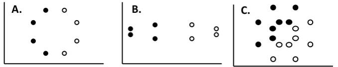
The Simplicity model (Pothos & Chater, 2002) is a model of unsupervised
categorization. It is the first model specifically developed to explain category intuitiveness,
that is, to explain why certain classifications for a set of concurrently presented stimuli
appear more natural to naïve observers than others. It assumes that preferred classifications
will involve groupings that maximize within-category similarity and minimize
between-category similarity, across all exemplars (see also Rosch & Mervis, 1975). Thus, like
SUSTAIN, the simplicity model instantiates a preference for similarity-based groupings in
unsupervised categorization. However SUSTAIN, unlike the simplicity model, has a bias
towards groupings using a subset of the stimulus dimensions.
The simplicity model aims to predict the optimal number of categories in an
unsupervised classification. It achieves this through a scheme for computing the codelengths
for the similarity information between the items, with and without categories (the particular
framework employed is Minimum Description Length, Rissanen, 1978). The codelength for
similarity information with categories can be lower than the codelength without categories, if
the categories can provide an efficient way of coding for this similarity information. Whether
this is possible or not clearly depends on how categories can code for similarity information
and the particular assumption in the simplicity model is that a category is a set of objects for
which all within-category similarities are greater than any between-category similarity
(following Rosch & Mervis, 1975). If the similarity structure of a set of objects is consistent
corresponding similarity information. Note that the assumption of how categories code for
similarity information is analogous to the specification of prior distributions in Bayesian
approaches (cf. Chater, 1996).
The simplicity model assumes that the optimal number of categories appropriate for a
set of objects is the number that reduces the codelength for describing similarity information
for that set of objects the most. Also, the difference between the codelength with categories
and the codelength without categories is a measure of the intuitiveness of the category
structure. The latter is the unique contribution of the simplicity model, as no other model can
immediately produce a value that can be interpreted as psychological intuitiveness (and
indeed this has been a dependent variable neglected in categorization research). Having a
quantitative measure of category intuitiveness can be very useful. For example, it allows the
model to make parameter-free predictions about dimensional attention (Pothos & Close,
2008; cf. Colreavy and Lewandowsky, 2008).
The simplicity model’s use of information theory comes at a price: the model has to
assume a non-metric space, so that similarity information is represented in terms of relative
magnitudes of similarities. This implies that, as long as categories are well separated, the
degree of separation does not matter and also the spread of categories does not matter. These
are important assumptions regarding the implementation of the simplicity model which have
yet to be confirmed.
Rational model
The Rational Model of Categorization (RMC; Anderson, 1991) is a trial-by-trial
model of categorization, based on Bayesian updating of probabilities. Specifically, it
determines the classification of a novel instance in terms of how likely the instance’s features
are, given the observed features of the members of different categories. As a result, the RMC
the simplicity model, RMC has a free parameter that determines how dissimilar a new
stimulus has to be to in order for it to form a new cluster. However, in SUSTAIN, this free
parameter only applies to unsupervised categorization, whilst in the RMC, it applies to both
supervised and unsupervised categorization. Also, like SUSTAIN, the RMC is able to
provide an account of both categorization and feature inference. One way in which attentional
selection can be implemented in the RMC is in terms of prior biases for particular dimensions
(Anderson, 1991; for an alternative approach see Pothos & Bailey, 2009).
One aspect that the RMC shares with the GCM is that the RMC has formed the basis
of a number of developments and related models. For example, Anderson and Matessa (1992)
proposed a modification to account for people’s sensitivity to feature correlations, and
Sanborn, Griffiths and Navarro (2006) have proposed a variant that allows order-independent
classification predictions.
Summary
The formal modeling of categorization is currently characterized by considerable
diversity - these models differ on most aspects it would be possible for categorization models
to differ. For example, the nature of intermediate representations (prototypes, exemplars,
adaptive clusters, fixed radial basis units), the nature of selective attention, single vs. multiple
systems approaches, feed forward vs. recurrent information flow, pick-the-best versus ratio
rule (Equation 1) decisions, similarity-based versus Bayesian classification. Those aspects of
the models for which there is consensus, or at least some convergence, tend to be constructs
from outside categorization research, and about which the formal modeling of cognition as a
whole has largely converged (e.g. adaptation as being driven by the minimization of
prediction error – see Friston, 2010, for the wide applicability of this concept).
This high degree of divergence amongst formal models of categorization obviously
empirical tests between different models. Moreover, it is hard to see these multiple models as
complementary. In order for them to be complementary, there would have to be consensus on
the situations in which each is best applied. This does not exist.
Reflecting on the arguments we made in favor of formal modeling, one might
reasonably argue that formal modeling of categorization has led to an increased appreciation
of the complexity of the problem, and also some deeper insight into empirical phenomena.
However, the presence of multiple, domain-general, models subverts many of the other
advantages of formal modeling – having multiple domain-general models does not serve the
goals of ambiguity reduction or behavior prediction (except, of course, in the special case
where all models behave in the same way). The way to rectify this problem is to make use of
the other main advantage of formal models – their ability to facilitate theory comparison
against empirical data. In the next section, we evaluate current practice in model comparison
within the field of categorization research, and make a series of best-practice
recommendations designed to maximize the chances for further progress. The issue of model
comparison is clearly pertinent for many areas of psychology, including areas with a close
relation to categorization such as recognition memory (Nosofsky & Stanton, 2006) and
magnitude estimation (Bergert & Nosofsky, 2007); however, the specific examples upon
which we draw in this article are from studies of categorization.
Model comparison
Model comparison, as defined here, is the comparison of at least two different classes
of model that have some currency in the literature, where the comparison concerns the
relative adequacy of those models to account for certain empirical phenomena. One example
of this kind of model comparison is the work by Nosofsky and Stanton (2005). In that paper,
account for the effects of probabilistic versus deterministic feedback on the accuracy and
speed of categorization. An exemplar model provided the best account of these data.
In contrast, research that evaluates the ability of a single model to encompass certain
phenomena does not constitute model comparison as defined here. For example, Nosofsky
and Palmeri (1996) present a demonstration that the ALCOVE model can accommodate the
results of a variant of the Shepard et al. (1961) experiment (see Figure 1) in which the
stimulus dimensions are integral (rather than separable, as in the original demonstration).
Such modeling work has considerable merit – it shows, for example, that there is at least one
extant model that can account for what has been found. Nevertheless, work of this type seems
unlikely to resolve the problem of multiple, divergent, non-complementary formal models of
categorization, which is the focus of the current article.
Similarly, comparing variants of the same class of model is undoubtedly important in
the development and refinement of a particular theoretical approach, but does little to solve
the central problem of multiple, divergent, non-complementary models. For example,
Nosofsky and Kruschke (1992) report (amongst other things) a comparison of the GCM
model with a subsequent development of the GCM. Work of this type is useful in the sense
that it helps motivate the development of models within a particular class, but does not
directly address the problem of resolving relations between divergent, non-complementary,
classes of model. A similar point pertains to comparisons where one model is
well-established, but the comparison model has no currency in the literature, and the less-well
established model is found to be inferior. Such comparisons have their uses, but they seem
unlikely to resolve the problem we consider here.
There are numerous positive examples of model comparison in the categorization
literature. For example, exemplar models have been compared against configural-cue models
Minda, 2000), the Rational model (Nosofsky et al., 1994; Pothos & Bailey, 2009), and
decision-bound models (McKinley & Nosofsky, 1996; Nosofsky & Palmeri, 1997b; Little,
Nosofsky & Denton, 2011). And yet, limited progress appears to have been made in reducing
the number of divergent, non-complementary models of categorization. Decision-bound
models have been around in something approaching their current form for more than 20 years
(Ashby & Gott, 1988), yet are still the subject of evaluation in current research (e.g. Little et
al., 2011). Configural-cue models have also been a feature of categorization research for
more than 20 years (e.g. Gluck & Bower, 1988) yet some of their key processing and
representational assumptions live on in models such as KRES. Prototype models of
categorization have been with us for at least 40 years (e.g. Reed, 1972), but still motivate
current research (e.g. Homa, Hout, Milliken & Milliken, 2011). Why the apparent lack of
confident progress towards reducing the number of divergent, non-complementary models of
categorization?
One possibility is that, as these are all very complex models and as principled
comparisons pose profound empirical, computational, and theoretical challenges, overall
progress is inevitably slow. No doubt, this is part of the answer. Another possibility, and the
one we explore in this article, is that progress is slower than it needs to because formal model
comparisons in categorization have generally been rather narrow. For example, Smith and
Minda (2000) presented an analysis comparing the GCM, the NSM prototype model, and
variants thereof, against many replications of a study that examined response probabilities for
a set of test items subsequent to training on one particular category structure (the “5-4”
structure, introduced by Medin & Schaffer, 1978)3. Hence, the comparison was restricted not
just to the same kind of evidence (classification probabilities) but effectively to variants of
the same data set. Pothos and Bailey (2009) explored the ability of three different models (an
different data sets. While initially promising, as it turned out, none of the models were clearly
superior across all five data sets, showing that a low ratio of data sets to models (5:3) was not
adequate to discriminate between these models (equally, that the particular data sets were
non-diagnostic in this comparison).
There are numerous other examples where model comparison has been restricted to
one or two experiments (e.g. Little et al., 2011; McKinley & Nosofsky, 1996; Nosofsky,
Kruschke & McKinley, 1992; Nosofsky et al., 1994; Nosofsky & Palmeri, 1997b; Nosofsky
& Stanton, 2005; Stanton, Nosofsky & Zaki, 2002). One might argue that narrow
comparisons are the result of what can reasonably be achieved in a single research article. No
doubt there is some truth in this argument, and researchers in the categorization field do
appreciate the necessity for broader comparisons. However, narrow comparisons are not
unavoidable in a general sense. For example, in the modeling of reading aloud, Perry, Ziegler
and Zorzi (2007) compared three models against thirteen benchmark phenomena. In the final
section of the current paper, we return to the issue of the extent to which broad comparisons
are feasible.
We start from the, in principle, non-controversial point that a key goal for formal
modeling must be to assess the relative adequacy of the numerous pre-existing models
against a broader range of the known empirical phenomena - to not do so is to essentially
negate most of the reasons for favoring formal models in the first place. In the current article,
we consider the ways in which a formal model can be assessed against empirical phenomena
and consider some of the reasons that have led to narrow model comparisons. Then, we
identify the approaches in the literature that we consider to be the gold standard for model
evaluation and development. We also list the range of DVs and IVs against which formal
models of categorization could reasonably be expected to be assessed. Even though all these
think it is important to summarize them here, as in practice model comparison has been
restricted to a handful of variables.
Assessing relative adequacy
Returning to our earlier definition, a formal model transforms changes in one or more
IVs into changes in one or more DVs. If model X does this better than model Y, model X
should be preferred over model Y – but how should relative adequacy be operationalized?
Below, we make the case that relative adequacy should be assessed by comparing
well-defined models on the basis of the number and proportion of irreversible, ordinal, penetrable
successes in accounting for empirical phenomena. Each of the components of this
operationalization of relative adequacy is discussed in the sections that follow.
Ordinal adequacy
One way to assess the empirical adequacy of formal categorization models is to
evaluate their ability to minimize the quantitative difference between their outputs and some
empirical observations. We describe this as SSE adequacy (SSE is an acronym for sum of
squared errors, a common measure of quantitative difference). Assessing formal models
solely on the basis of SSE adequacy has two serious problems:
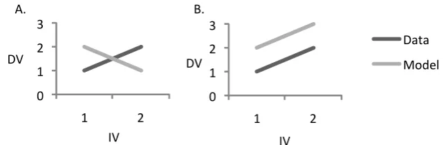
(1) SSE does not distinguish between quantitative and qualitative adequacy, as
illustrated in Figure 5. On an SSE measure, the two models in Figure 5 are indistinguishable
– they have the same SSE. Yet, most theorists would agree that the model in Figure 5B
provides a better account of the empirical results than the model in Figure 5A. This is
because the model in Figure 5B correctly predicts that increases in the IV lead to increases in
the DV, whilst Figure 5A makes the opposite prediction.
(2) A reliably lower SSE is not necessarily indicative of a more adequate model.
Indeed, except in the purely theoretical case where measurement error is zero, the model with
the lower SSE can sometimes be the less adequate model, if its lower SSE comes from its
greater ability to fit noise. This phenomenon is described as overfitting.
Overfitting can be revealed by techniques such as cross-validation – one splits the
data into a calibration and a validation sample (typically, the calibration and validation
samples are two random subsets of the responses made by a participant). The model
parameters are estimated via minimization of SSE on the calibration sample, and then the
same parameters are applied to the validation sample. The greater the increase in SSE from
the calibration sample to the validation sample, the more likely it is that the model overfitted
the calibration sample.
Overfitting is a real possibility in the formal modeling of categorization. For example,
Minda and Smith (2001) argued that a prototype model provided a better account of a
particular set of data than an exemplar model on the basis of a small difference in quantitative
fit (the prototype model was closer to the data by about three percentage points on average).
In a replication that included cross-validation analysis, Olsson Wennerholm and Lyxzen
(2004) demonstrated that the prototype model showed a greater increase in SSE from
calibration to validation sample than did the exemplar model, with both models showing the
same level of fit in the validation sample. This raises the possibility that the superior
quantitative fit of the prototype model in the calibration sample (and, by extension, in Minda
and Smith, 2001) was due to overfitting. Nosofsky and Zaki (2002) also queried the Minda
and Smith’s (2001) results, noting that where the GCM exemplar model included a
response-scaling parameter (γ in Equation 1), it could accommodate Minda and Smith’s results better
than a prototype model. However, Olsson et al. (2004) demonstrated that the version of GCM
calibration to validation sample, than did a version of GCM not including a response-scaling
parameter (with both versions of GCM producing equivalent levels of fit in the validation
sample). This again illustrates the potential for overfitting in the comparison of formal
models of categorization. Of course, the issue of whether the inclusion of a gamma parameter
leads to overfitting in the narrow comparison of three models to one experiment is different
to the issue of whether the GCM (or any other model) requires a gamma parameter in order to
be able to accommodate a broader range of results.
In summary, SSE is dissociated from important aspects of relative adequacy – two
models can have the same SSE in cases where most theorists would agree one is superior, and
better SSE can sometimes indicate a less adequate model. For both these reasons, we argue
that the primary evaluation of formal models of categorization should be against a criterion of
ordinal adequacy. In other words, we are suggesting that models should primarily be
assessed first as to whether they capture the ordinal properties of a data set. For example, in
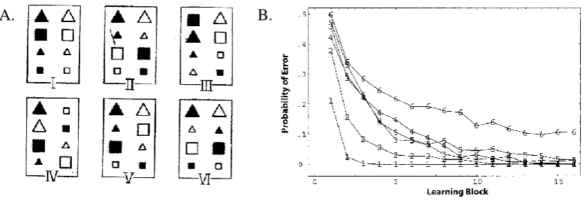
the Shepard et al. (1961) data set (see Figure 1), this might mean getting the six problem
types in the correct order of difficulty. Assessing adequacy by the ability to reproduce the
ordinal properties of a data set eliminates the problem described in Figure 5 – the model in
Figure 5B is the more adequate account under a criterion of ordinal adequacy. Adopting
ordinal adequacy as the primary measure of success also reduces (but does not necessarily
eliminate) the risks of illusory model superiority due to overfitting.
An ordinal adequacy criterion does not limit models to simple findings – one could
assess, for example, whether a model could reproduce the ordering of the curvatures of a
category acquisition function, or the kurtosis of a set of RT distributions. And making ordinal
adequacy primary does not render SSE redundant. Where, across a broad range of
SSE provide a useful secondary measure of model adequacy (as do Bayesian methods of
model selection, e.g. Boucher & Dienes, 2003; Pitt, Kim & Myung, 2003).
There are cases in the literature that include assessments of ordinal adequacy,
including many of those we referred to in the earlier discussion of our definition of model
comparison. For example, in Nosofsky et al. (1994), GCM is shown to make an ordinally
different prediction to certain configural-cue models (Gluck & Bower, 1988), with the data
being consistent with the GCM’s predictions. Similarly, in Nosofsky and Palmeri (1997b),
the EBRW model is shown to make an ordinally different prediction to a decision-bound
model, with the data being consistent with the EBRW model.
There are also cases where model comparison has proceeded solely on the closeness
of quantitative fit, with both models being able to accommodate the ordinal pattern observed.
For example, McKinley and Nosofsky (1995) concluded in favor of a variant of the GCM
model (over a decision-bound model) solely on the basis of degree of quantitative fit.
Similarly, Shin and Nosofsky (1992) report a comparison in which GCM accounted for 98%
of the variance whilst the prototype model accounted for 94% of the variance.
In summary, some model comparisons in categorization research have included
ordinal success as part of their evaluation, whilst others have relied solely on the quantitative
closeness of fit. Our argument is that comparisons that include a consideration of ordinal
success represent best practice, for the reasons outlined above. Of course, regardless of
whether evaluations are based solely on SSE, or whether they additionally include
consideration of ordinal success, it remains important that models provide an account of as
much as the collected data as possible, rather than focusing on one or two collected data
Functions of quantitative adequacy
To clarify, we are not advocating a complete avoidance of a quantitative approach to
model evaluation. We believe quantitative adequacy, when considered in combination with
ordinal success, can serve important functions. For example, whilst the focus of the current
article is on formal model comparison, this is not the only way in which formal models can
be employed. Another use of formal models is as an existence proof that a particular model
has the potential to encompass a particular result. One example of this approach is Nosofsky
and Zaki’s (1998) demonstration that a version of GCM can account for the fact that
amnesics are sometimes more impaired on old-new recognition than they are on
categorization (Knowlton & Squire, 1993), a result previously considered to be outside the
scope of single-system theories. The impact of such existence proofs seems to be increased if
the formal model captures not only the ordinal patterns of the experiment, but also provides a
striking degree of quantitative closeness. The issue of what degree of closeness is required to
be sufficiently impressive is, of course, rather vague in situations where only one formal
model is considered. Nevertheless, it is beyond dispute that quantitatively close existence
proofs can have a profound impact on the field (as measured by, for example, the number of
citations they receive).
Another potential use for quantitative adequacy is in situations where all models
under comparison capture the ordinal patterns in the data. Under such circumstances, one
may wish to favor the model that produces the closest overall quantitative fit. In situations
where one is confident that the difference in quantitative fit does not result from overfitting
(see above), closeness of quantitative fit may provide some useful additional information,
both in terms of relative model success and in terms of estimation of parameter values (as
parameter values can provide information about how models account for an empirical
of quantitative fit – the latter takes into account the magnitude of effects whilst the former
does not. It is conceivable that, as the comparison of models against a broad set of data
proceeds, a trade-off will emerge where Model X accounts for more ordinal patterns than
Model Y, but at the expense of having lower quantitative adequacy than Model Y. The issue
of which model is the more adequate under these conditions would rightly be a topic for
serious debate, and a measure of quantitative adequacy would clearly be necessary to inform
that debate.
Irreversible success
We argued earlier that one of the main advantages of formal models over more
informal forms of theorizing was the potential of formal models for ambiguity reduction. We
also argued that one reason this potential had failed to be realized in the formal modeling of
categorization was the presence of multiple domain-general models and no consensus on the
relative adequacy of these models. Here, we emphasize that achieving progress towards
consensus requires an avoidance of arbitrarily variable parameters, and an evaluation of the
relative adequacy of models through an examination of the irreversiblesuccesses that can be
attributed to them. Below, we provide a definition of the concept of arbitrarily variable
parameters, illustrate why they are a problem, and propose the assessment of relative
adequacy through irreversible modeling successes.
Arbitrarily variable parameters
A model parameter is some (usually numerical) information that is part of the model
specification, rather than provided via the IV inputs. Most models have parameters, including
some of the most successful and elegant formal models ever created (e.g. Newtonian gravity).
Having parameters, even a large number of parameters, does not in itself cause any problems
In the formal modeling of cognition, the term free parameter is in common usage. We
define a free parameter as any parameter whose value is determined as part of the process of
determining model adequacy. Determining optimal values for free parameters can be seen as
part of the process of model development, and the presence of free parameters has no
necessary consequences for model ambiguity – as long as the values of those parameters are
universal. Universal free parameters are those whose specification is general to the whole
domain of phenomena that the model is intended to address. By contrast, an arbitrarily
variable parameter is one that can take different values for different levels of an independent
variable, and where each of those values is determined through a process of maximizing
model adequacy (as opposed to, for example, being determined by independently measurable
properties of the stimulus, environment or participant).
The problem of arbitrarily variable parameters
Allowing parameters to take freely determined values for different levels of an IV can
cause severe ambiguity if changes in the value of that parameter are able to cause ordinal
changes in the model’s output. For example, Wills, Suret and McLaren (2004) examined
whether pre-exposure to two different stimulus types facilitated or retarded subsequent
categorization of those stimuli. Let’s consider the IV here to be stimulus type (two levels –
noise distorted vs. re-arrangement distorted) and the DV to be the direction of the exposure
effect (two levels – retardation or facilitation). On that basis, four ordinally different things
could have happened – of course, only one actually did (noise-distorted stimuli were
facilitated; re-arrangement-distorted stimuli were retarded). One approach to modeling this
experiment with the GCM would have been to allow c (the parameter controlling the overall
expansion of psychological space, see Figure $C) to take four different values, one for
pre-exposed noise-distorted stimuli, one for non-prepre-exposed rearrangement-distorted stimuli, and
accommodated by the GCM. But so could the three other possible results of this experiment
that were not found. Indeed, the use of arbitrarily variable parameters in this case leads the
GCM to become what is described as a degenerate model (Smith, Chapman & Redford,
2010)4.
An alternative approach to modeling the results of Wills et al. (2004) with the GCM
would be to use as input to the GCM psychological spaces derived from similarity ratings
taken both before and after pre-exposure. This might capture the representational changes
that result from exposure, and might have allowed the GCM to fit the data with a single set of
parameters for all four conditions. Such an approach does not provide an account of
representational change, but it (a) provides a clear statement that the form of representational
change observed in Wills et al. (2004) is outside the explanatory scope of the GCM, and (b)
removes arbitrarily variable parameters from the model specification in this context. For both
these reasons, this second application of GCM is more useful in assessing model adequacy
than the first application5.
Defining irreversible success
The second application of GCM, if it worked, would also be an example of a model
without arbitrarily variable parameters – but only in the microworld of the experiment
discussed. Absence of arbitrarily variable parameters must properly be defined across the
entirety of the data sets to which a model is applied – not just the context of a single study.
An ordinal success in reproducing the effects of IVs on DVs, in the absence of
arbitrarily variable parameters, is what we describe as an irreversible success. The success is
irreversible in the sense that turning one particular success into a failure (or, perhaps more
appositely, a failure into a success) cannot be done without re-evaluating the model’s ability
to fit the entire data set that defines the model’s domain. Derivation of a model’s parameters
derivation of these parameters for each experiment (or even each condition of each
experiment), ensures the model’s successes are irreversible in the sense we have defined it
here.
Number of empirical successes
A model that accommodates more of what we know empirically is, other things being
equal (see later sections), a better model. Hence, our proposal is that relative adequacy of
formal models can be assessed on the basis of the number of irreversible ordinal successes
that can be attributed to them. This proposal contrasts sharply with current practice in
categorization research, which is to examine in depth the results of a single or a handful of
experiments, rather than seek breadth. For example, the original publication of GCM
(Nosofsky, 1984) assessed the model against the result of just one, at that point unreplicated,
study with six participants (Shepard et al., 1961). Twenty years later, the original publication
of SUSTAIN (Love et al., 2004) assessed the model against seven experiments. One
commendable aspect of the original assessment of SUSTAIN was that it employed universal
free parameters – in other words, parameters that had a common value across all seven
studies. SUSTAIN therefore achieved 7 irreversible ordinal successes in its original
publication.
Both GCM and SUSTAIN have subsequently been assessed against other data.
However, in both cases, these assessments have largely been performed independently of the
original assessments. In other words, subsequent publications have determined the value of
the model’s parameters on the basis of maximizing the model’s ability to reproduce the
results of the particular studies considered in that paper. Against the criteria we are
proposing, these additional publications do not necessarily demonstrate an increase in the
number of irreversible ordinal successes of the model, and therefore do not necessarily reflect
examples, we do not intend to imply that these problems are specific to those models, or even
that they are specific to models of categorization (for a related argument in the formal
modeling of perception, see Pitt et al., 2003, p. 30).
One way to have met the proposed criteria would have been to determine the values
of free parameters by their ability to maximize the number of ordinal successes across the
combined data set – in other words, all studies against which the model had previously been
compared, plus the additional data being considered in the new paper. Of course, it may be
the case that different data sets will require different values for the model’s parameters. As
previously stated, a model with a large number of parameters is not necessarily ambiguous –
what matters is whether those parameters are arbitrarily variable. For example, the
attentional parameters in Nosofsky’s (1984) fit of the GCM to the data of Shepard et al.
(1961) are not arbitrarily variable because they are constrained by the hypothesis that
dimensional attention is allocated to maximize categorization accuracy (a hypothesis
subsequently given a formal mechanism in the ALCOVE model). This hypothesis results in
the attentional parameters of GCM taking different values for the different conditions of
Shepard et al. (1961). However, this variation is not arbitrary – in fact, it means that there are
essentially zero free parameters for attention in that application of GCM.
As an illustration of the shortcomings of evaluating results in isolation, consider the
work of Medin and Schaffer (1978). In one of the most influential results in the early
development of exemplar theories, Medin and Schaffer demonstrated that, within the
category structure shown in Figure 6, participants learned to respond correctly to stimulus A2
more quickly than they learned to respond correctly to stimulus A1. This occurred despite the
fact that the features of A1 are in some sense more typical of Category A members than are
the features of A2. Note that properties denoted “1” in Figure 6 are characteristic of Category