Solar sail dynamics in the three-body problem: homoclinic paths of points and orbits

Solar sail dynamics in the three-body problem:

homoclinic paths of points and orbits

Thomas J. Waters and Colin R. McInnes

Department of Mechanical Engineeering, University of Strathclyde, Glasgow

Abstract

In this paper we consider the orbital dynamics of a solar sail in the Earth-Sun circu-lar restricted 3-body problem. The equations of motion of the sail are given by a set of nonlinear autonomous ordinary differential equations, which are non-conservative due to the non-central nature of the force on the sail. We consider first the equilibria and linearisation of the system, then examine the nonlinear system paying partic-ular attention to its periodic solutions and invariant manifolds. Interestingly, we find there are equilibria admitting homoclinic paths where the stable and unstable invariant manifolds are identical. What’s more, we find that periodic orbits about these equilibria also admit homoclinic paths; in fact the entire unstable invariant manifold winds off the periodic orbit, only to wind back onto it in the future. This unexpected result shows that periodic orbits may inherit the homoclinic nature of the point about which they are described.

1 Introduction

A soalr sail is a novel type of spacecraft which uses the radiation pressure of photons reflecting off large sails as its impulse (see McInnes [13] for a detailed description). A natural setting for the solar sail is the circular restricted 3-body problem (CR3BP) where the Earth and the Sun are the primary bodies. This is partly because the 3-body problem more accurately describes solar system dynamics than the 2-body problem, but also because in the 3-body problem there are regions where the gravitational forces on the sail due to the primaries cancel each other, and hence the radiation pressure force on the sail plays a more dominant role. Also, the demands on sail efficiency would be less as the gravitational forces are less, and thus the applications of this analysis are more in the near-term.

we will follow in this paper. In particular we will direct our attention to the nonlinear system’s periodic orbits and invariant manifolds. There has been some work carried out on the dynamics of solar sails in the CR3BP. McInnes et al. [14] first described the surfaces of equilibrium points, and some possible uses of same. In Baoyin and McInnes [1] and McInnes [12], the authors describe periodic orbits about equilibrium points in the solar sail three body problem, however they consider only equilibrium points on the axis joining the primary masses, corresponding to artificial Lagrange points. Such orbits are analogous to the classical ‘halo’ orbits (where by classical we mean the particle is only acted upon by gavitational forces), which are well documented, for example Farquhar [4], Farquhar and Kamel [5], Breakwell and Brown [3], Richardson [15], Howell [9] and Thurman and Worfolk [18]. With regards to the invariant manifolds, there has been much analysis of the invariant manifolds of halo orbits in the classical problem for the sake of efficient transfer; for example the Genesis mission trajectory was designed using this technique (see Koon et al. [10]), and a ‘petit grand tour’ of Jovian moons has been proposed using a similar analysis (see G´omez et al. [6]). Some homoclinic paths for the classical triangular points have been found for large mass ratios (see for example G´omez et al. [7]), and homoclinic paths can exist for collinear points with particular mass ratios (see §9.9.2 of Szebehely [16]). Certain isolated homoclinic paths have been found for periodic orbits about the collinear Lagrange points (see for example Koon et al. [11]), however no periodic orbit whose invariant manifold is made up entirely of homoclinic paths has been found, to the best of our knowledge.

The structure of the paper is as follows: in the next section we will describe the setting of the problem and the equations of motion of the solar sail, as well as the equilibrium points. Section 3 considers the system linearised about equilib-rium and the form of the linear solutions. In Section 4 we briefly describe the Lindstedt-Poincar´e perturbation method used to find nonlinear approxima-tions to periodic orbits, and in Section 5 we examine the invariant manifolds of equilibria and periodic orbits. We find a large variety in the position, in-clination, amplitude and frequency of periodic solutions to the equations of motion, and unexpected homoclinic paths associated with equilibria and pe-riodic orbits which have no analogue in the classical problem. Such results suggest that the solar sail CR3BP presents a rich and complex model, the intricate details of which are only beginning to become apparent.

2 Equations of motion in the rotating frame

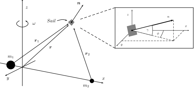
-axis completes the triad. We chose our units to set the gravitational constant, the sum of the primary masses, the distance between the primaries, and the magnitude of the angular velocity of the rotating frame to be unity. We shall denote by µ = 3×10−6

the dimensionless mass of the smaller body m2, the

Earth, and therefore the mass of the larger bodym1, the Sun, is given by 1−µ

(see Figure 1).

Denoting by r,r1 and r2 the position of the sail w.r.t. the origin,m1 and m2

respectively, the solar sail’s equations of motion in the rotating frame are

d2

r

dt2 + 2ω×

dr

dt =a−ω×(ω×r)− ∇V ≡F, (1)

with ω = zb and V =−[(1−µ)/r1+µ/r2] where r_i =|r_i|. These differ from

the classical equations of motion in the CR3BP by the radiation pressure acceleration term

a=β(1−µ) r2

1

(rb1.n) 2

n, (2)

where β is the sail lightness number, and is the ratio of the solar radiation pressure acceleration to the solar gravitational acceleration. Herenis the unit normal of the sail and describes the sail’s orientation. We definenin terms of two angles γ and φ w.r.t. the rotating coordinate frame,

n= (cos(γ) cos(φ),cos(γ) sin(φ),sin(γ)), (3) where γ, φ are the angles the normal makes with the x-y and x-z plane re-spectively (see Figure 1).

Equilibria are given by the zeroes of F in (1). We find a 3-parameter family of equilibria, as described in McInnes [13]. These are found by specifying the lightness number β and the sail angles γ and φ, and solving F = 0 for one of

z

x y

r₁

r₂ r

n

m2

m1

Sail ω

γ φ

x

y z

n

Fig. 1. The rotating coordinate frame and the sail position therein. The anglesγ and

0.985 0.99 0.995 1 1.005 1.01 -0.015 -0.01 -0.005 0 0.005 0.01 0.015

0.985 0.99 0.995 1 1.005 1.01 -0.015 -0.01 -0.005 0 0.005 0.01 0.015 b

c bc bc

L1 L2

Earth β= 8 > > > < > > > :

0_.03 0.05 0_.1 0_.2 0.4

xe ze

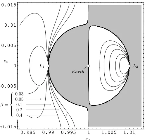
Fig. 2. Surfaces of equilibrium points in the xe-ze parameter space. Each curve is

specified by a constant value of β, and the position of the equilibrium point along the curve is given byγ. The grey shaded regions denote areas where equilibrium is not possible.

two possible equilibria, one on the L1 side and another on the L2 side of the

Earth. For reasons we shall describe in the next section we will take φ= 0 so the equilibrium (and sail normal) is in thex-z plane. In Figure 2 we show some of the equilibria near the Earth for low β values. Practically speaking, while a β value of about 0.3−0.4 is considered within the realm of possibility of current engineering, to put the analysis in this paper well within the near-term we will consider very modest β values of about 0.05.

3 Linearised system

We linearise about the equilibrium point (in the x-z plane) by making the transformation r → re +δr, Taylor expanding F about re, and neglecting

the terms quadratic in δr. We assume the orientation of the sail will remain fixed under perturbation of the sail position, in which case γ, φ and β are constants. Lettingδr = (δx, δy, δz)T _{and X = (δr, δr˙)}T_{, our linear system is}

˙

X =AX with

A=

   0 I

M Ω

 

, M =       

a 0 b

0 c 0

d 0 e

      

, Ω =

      

0 2 0

−2 0 0

0 0 0

where a dot denotes differentiation w.r.t. t,

a= (∂xFx)|e, b = (∂zFx)|e, c= (∂yFy)|e, d= (∂xFz)|e, e= (∂zFz)|e,

and b6=d. HereFa _{denotes the a-th component ofF, andM is sparse due to}

ye = 0.

The key difference between this analysis and the classical orbits about the collinear Lagrange points is the term d 6= 0, which appears precisely because we are linearising about an equilibrium point with ze 6= 0. This means we

cannot decouple thez-equation. While this initially seems to make the problem more complicated, we can use this to our advantage, as will be made clear.

The characteristic equation of the JacobianAis bi-cubic (whose corresponding cubic equation has real roots); this means the eigenvalues of A are either in pairs of pure imaginary conjugates or real and of opposite sign. Thus equilibria in thex-z plane will have the dynamical structure of centres and saddles, akin to the classical collinear Lagrange points; in fact we find the linear spectrum

to be typically _n

λ1i,−λ1i, λ2i,−λ2i, λ_r,−λ_r o

. (5)

Had we chosen φ 6= 0 for an equilibrium out of the x-z plane, then M given in (4) would be full and the characteristic equation would not have been bi-cubic; thus the dynamical structure of equilibria out of the x-z plane will be stable/unstable spirals and saddles. In fact, equilibria in thex-yplane (γ = 0,

φ 6= 0) will be stable spirals crossed with saddles for φ < 0 (ye < 0) and

unstable spirals crossed with saddles for φ > 0 (ye > 0). In this sense the

x-axis is a bifurcation surface.

If we label the eigenvectors associated with λai (a = 1,2) as ua+wai, and

the eigenvectors associated with λr,−λr as v1,v2, then the general solution

of the linear system (4) is [2]

X(t) = cos(λ1t) h

Au1+Bw1 i

+ sin(λ1t) h

Bu1−Aw1 i

+ cos(λ2t) h

Cu2 +Dw2 i

+ sin(λ2t) h

Du2−Cw2 i

+Eeλrt

v1 +F e−λrtv2. (6)

We see that due to the coupling of thez-equation in the linear system, which in turn is due to our choice ofze 6= 0, the linear order solution naturally contains

periodic solutions in both _{linear frequencies. By setting E = F = 0 we may}

switch off the real modes, and by setting either A=B = 0 or C =D= 0 we have periodic solutions in the frequency of our choice.

While these trajectories will not in general close, by choosing an equilibrium point whose linear frequencies are in ratio we may find multiply periodic or-bits, however this raises some stability issues. We will not pursue such orbits in this paper.

4 High-order approximations to periodic orbits

The linear solutions given in the previous section will only closely approximate the motion of the sail given in (1) for small amplitudes. For larger amplitude periodic orbits, we have two options: nonlinear analytical approximations or numerical continuation of initial data. While numerical continuation is the most straightforward and can be continued beyond the region where the lin-ear term dominates, it is a slow process and needs to done for each equilibrium point of the 2-parameter family separately. The nonlinear analytical approxi-mations will quickly provide converging initial data for large amplitude orbits at arbitrary equilibria, and so is to be preferred in the region where the linear term dominates. To calculate high-order approximations to periodic orbits we use the method of Linstedt-Poincar´e. This procedure is well known and is described in the literature, for example [15,18], thus we will only outline the relevant issues for this model.

We let ε be a perturbation parameter and expand each coordinate as x →

xe+εx1 +ε 2

x2 +. . . etc. We rescale the time coordinate τ = ωt with ω =

1 +εω1 +. . ., and group together the powers of ε in the high-order Taylor

expansion ofF. We choose our linear solution to be

x1 =kA_ycos(λτ +ξ), y1 =A_ysin(λτ +ξ), z1 =mA_ycos(λτ +ξ),(7)

where λ can be λ1 or λ2, k, m are given in terms of components of the

eigen-vectors and Ay, ξ are free parameters (we have set the y-amplitude to be the

free parameter to avoid singularities in the coefficients when the orbits pass through vertical or horizontal). We use these linear solutions to build up non-linear approximations to periodic orbits one order at a time in the following way:

At each order of ε, the system to be solved will be

x′′

n−2yn′ −axn−bzn=g1(xn−1, yn−1, zn−1, xn−2, . . .)

y′′

n+ 2x′n −cyn =g2(x_n−1, y_n−1, z_n−1, x_n−2, . . .)

z′′

n −dxn−ezn=g3(x_n−1, y_n−1, z_n−1, x_n−2, . . .), (8)

solutions act as forcing terms. We use the freedom in ωn to switch off the

resonant or secular terms in the inhomogeneous part, that is those compo-nents on the right hand side of the form (7), and what remains is a series of trigonometric subharmonics up to ordern.

In calculating the solution atnth order, we find two sets of solutions depending on whethern is even or odd. Whennis even, the nth order solutions have the form (letting T =λτ +ξ)

xn =pn0+pn2cos(2T) +. . .+pnncos(nT),

yn = qn2sin(2T) +. . .+q_nnsin(nT),

zn =sn0 +s_n2cos(2T) +. . .+s_nncos(nT), (9)

with ωn−1 = 0. When n is odd, the solutions at nth order have the form

xn = pn3cos(3T) +. . .+pnncos(nT),

yn =qn1sin(T) +q_n3sin(3T) +. . .+q_nnsin(nT),

zn =sn1cos(T) +s_n3cos(3T) +. . .+s_nncos(nT), (10)

and ωn−1 solves

2λβn1

(c+λ2

) +

bγn1

(e+λ2

) −αn1 = 0. (11)

Here αnj, βnj and γnj are the coefficients of the cos,sin and cos terms in the

functionsg1, g2 andg3 respectively at ordern given in (8), and the coefficients

pnj, qnj and snj are given by

−(a+j2

λ2

)pnj −2jλqnj−bsnj −αnj = 0,

qnj =

−2jλpnj−βnj

(c+j2

λ2

) , snj =

−dpnj−γnj

(e+j2

λ2

) , (12)

with the exception of qn0 = 0 and p_n1 = 0.

With these high order approximations, we may find approximate initial data from which to integrate the system of equations (1). However these will not evolve to exactly periodic trajectories, as they are only approximations to periodic solutions. Thus we must define a differential corrector with which to adjust the initial data so as to close the orbit. As differential correctors are discussed in much detail in the literature, particularly relating to the classical halo orbits (see for example [3,15,18]), we will not describe them here.

0.985

0.99

0.995

1 x

-0.0020 0.002 y

0 0.005

0.01 0.015

z -0.0020

0.002

0 0.005

0.01 0.015

L1

Earth

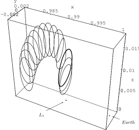
Fig. 3. A family of orbits withβ = 0.05. Each orbit has the same amplitude and is about a different equilibrium point along theβ level curve shown in Figure 2, each equilibrium point being defined by a differentγ value. For reference the Earth (to scale) andL1 are shown.

There is therefore much variety in the position, inclination, amplitude and pe-riod of the orbits we may describe, leading to a rich source of pepe-riodic orbits for various applications. To illustrate this, we may hold the amplitude fixed and allow γ to vary, thus forming a tube of periodic orbits along the β level curve. An example of this for one family of periodic orbits is shown in Figure 3.

5 Homoclinic paths

As a practical consideration it is useful to examine the transfer of a solar sail from Earth orbit to an equilibrium point. This is most easily accomplished by considering the equilibrium point’s invariant manifolds.

Letting r = (x, y, z)T _{and X = (r,r˙), we write the system (1) as ˙X =f(X)}

with equilibrium given by f(Xe) = 0. Let us denote by Eu,Es and Ec the

linear eigenspaces spanned by the unstable, stable and centre eigenvectors of the equilibrium point, that is those due to eigenvalues with positive, negative and zero real part respectively, and denotedv1,v2andu_a+iw_ain (6). From (5)

We will define the invariant manifolds Wu_,Ws _and Wc _{as those families of}

solutions to the non-linear system (1) which are tangential to Eu_,Es _and Ec

at the equilibrium point, with the property that

X(t0)∈W∗ ⇒X(t)∈W∗ ∀t,

that is, the manifolds are invariant under the flow.

These manifolds are of great practical importance as they characterise the dynamics of (1) away from the equilibrium point. For example, the centre manifold describes the surface on which periodic solutions exist, and the Lindstedt-Poincar´e method can be seen as calculating high-order approxima-tions to trajectories on the centre manifold. The stable and unstable manifolds characterise the flow onto and away from the equilibrium point, in particu-lar the unstable mode dominating the flow and pushing solutions away from equilibrium in the direction of the unstable manifold.

The true stable and unstable manifolds tend onto and away from the equi-librium point asymptotically. To avoid having to integrate the equations of motion for infinite lengths of time we must therefore approximate the invari-ant manifolds by perturbing the initial data a small amount away from the equilibrium point in the direction of the linear eigenvectors, and then inte-grate the system in this direction forward and backward in time. If we find a portion of the approximation to the stable manifold passes close to the Earth then this provides us with a potential efficient trajectory on which to transfer from the Earth to the equilibrium point.

Interestingly however, we find that there are certain equilibria on theL2 side

of the Earth which admit homoclinic paths; we define a homoclinic path as a phase path which joins an equilibrium point to itself. This means the stable and unstable invariant manifolds intersect smoothly and thus are identical. Equilibrium points admitting homoclinic paths are not to be confused with homoclinic points, which are points (other than the equilibrium point) where the stable and unstable invariant manifolds intersect transversally. Homoclinic paths occur for specific parameter values and are not structurally stable (in fact they represent a homoclinic bifurcation), unlike homoclinic points. See, for example, Tabor [17] for an introduction to homoclinic points/paths.

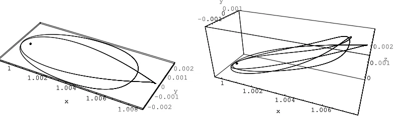
1 1.002 1.004 1.006 1.008 x -0.002 -0.001 0 0.001 0.002 y 1 1.002 1.004 1.006 1.008 x 1 1.002 1.004 1.006 x -0.001 00.001 y 0 0.001 0.002 z 1 1.002 1.004 1.006 x -0.001 00.001 0 0.001 0.002

Fig. 4. Homoclinic paths on theL2 side of the Earth. The trajectory shown is the (approximation of the) stable/unstable invariant manifold. The figure on the left has parameter values β = 0.015, γ = 0, φ = 0, while the figure on the right has

β= 0.05, γ = 0.7, φ= 0. The Earth is also shown.

We may also define the invariant manifolds of periodic orbits about equilibria in a manner analogous to above, using Floquet theory (see Grimshaw [8] for example). LetΓ(t) denote a periodic solution to (1), with periodT. By letting

X =Γ+Y, we may linearise the nonlinear system about this periodic solution, resulting in the variational equations

˙

Y = ∂f

∂X

¯ ¯ ¯

¯_X=ΓY ≡A(t) Y, (13)

whereA(t+T) =A(t). This is a non-autonomous linear system with periodic coefficients. A well known result of Floquet theory is that for every funda-mental solution matrix Y(t) of a system such as (13), there is a non-singular constant matrix B such that

Y(T) =Y(0)B. (14)

Therefore the eigenvalues of B tell us about the linear orbital stability of the periodic orbit. Recasting the variational equations in terms of the state transition matrix (or principal fundamental matrix) Φ =∂X/∂X(0), we have

˙Φ =A(t)Φ, Φ(0) =I,

and thus we asscociate the matrixB given in (14) with Φ(T), the monodromy matrix.

As the divergence of our original system vanishes, that is the trace of the Jacobian P∂fi_/∂X

i = 0 (see (4)), Louiville’s theorem (constancy of volume

approximations are valid), it follows that all of the periodic orbits described in this paper will be unstable, that is all monodromy matrices will contain two real reciprocal eigenvalues one of which will be larger than one. Complex conjugate eigenvalues must be on the unit circle and this represents a marginal stability, akin to eigenvalues of the Jacobian on the imaginary axis. Thus we find the spectrum of the monodromy matrix of the periodic orbits described in this paper to be

n

1,1, λi,λ¯i, λr,1/λr

o

, (15)

where an overbar denotes complex conjugacy.

Analogous to equilibrium points, we may integrate points along the periodic orbit in the direction of the eigenvectors of the monodromy matrix and find the trajectories which wind onto and off of the periodic orbit, that is the stable and unstable invariant manifolds of the periodic orbit. We find that the periodic orbits inherit the homoclinic characteristics of the equilibrium point about which they are described, and we show in Figure 5 an example of this for one of the equilibrium points in Figure 4. We see that every trajectory in the invariant manifold of the periodic orbit is itself a homoclinic path, and this persists for varying amplitudes of the periodic orbit.

6 Conclusions

In this paper we have presented an initial analysis of the periodic orbits avail-able to solar sails in the circular restricted three-body problem (CR3BP). We find there is a four parameter family of periodic orbits about equilibria in the

x-z plane (two due to choice of equilibrium point and two due to amplitudes in the linear frequencies). We have further examined the invariant manifolds of equilibria and periodic orbits, and have found unexpected families of homo-clinic paths. These homohomo-clinic paths suggest the model contains an interesting degree of complexity, perhaps akin to the R¨ossler attractor. There, homoclinic paths can be seen as a limit of multiply periodic orbits and this suggests that the solar sail model will contain many families of periodic orbits which pass close to the equilibrium point. This limit-type structure is seen also in the triangular points of the classical three-body problem. A more detailed ex-amination of the homoclinic and indeed heteroclinic paths contained in the problem should therefore be of interest.

1

1.002

1.004

1.006

x

-0.001

0

0.001

y

0

0.001

0.002

0.003

z

0

0.001

0.002

0.003

Fig. 5. A triply-periodic homoclinic invariant manifold of a periodic orbit about the equilibrium point with parameter values β = 0.05, γ = 0.7, φ = 0 (on the right in Figure 4). To give a sense of the flow the shading of the trajectory fades to grey with time.

References

[1] H. Baoyin and C. McInnes. Solar sail halo orbits at the Sun-Earth artificial L1 point. Celestial Mechanics and Dynamical Astronomy, (94):155–171, 2006.

[2] David Betounes. Differential Equations: theory and applications. Springer-Verlag, New York, 2001.

orbits in the Earth-Moon restricted 3-body problem. Celestial Mechanics, 20:389–404, 1979.

[4] R. Farquhar. The control and use of libration-point satellites. Ph.D. Dissertation, Stanford University, 1968.

[5] R.W. Farquhar and A.A. Kamel. Quasi-periodic orbits about the trans-lunar libration point. Celestial Mechanics, 7:458–473, 1973.

[6] G. G´omez, W.S. Koon, M.W Lo, J.E Marsden, J. Masdemont, and S.D. Ross. Invariant manifolds, the spatial three-body problem and petit grand tour of Jovian moons. Libration Point orbits and applications (Eds. G. G´omez, M.W. Lo and J. Masdemont), World Scientific, 2003.

[7] G. G´omez, J. Llibre, and J. Masdemont. Homoclinic and heteroclinic solutions in the restricted three-body problem. Celestial Mechanics and Dynamical Astronomy, 44(3):239–259, 1988.

[8] R. Grimshaw. Nonlinear ordinary differential equations. Blackwell Scientific Publications, 1990.

[9] K.C. Howell. Three-dimensional, periodic, ‘halo’ orbits. Celestial Mechanics, 32:53–71, 1984.

[10] W.S. Koon, M.W. Lo, J.E. Marsden, and S.D. Ross. The Genesis trajectory and heteroclinic connections.AAS/AIAA Astrodynamics Specialist Conference, Girwood, Alaska, (AAS99-451), 1999.

[11] W.S. Koon, M.W. Lo, J.E. Marsden, and S.D. Ross. Heteroclinic connections between periodic orbits and resonance transitions in celestial mechanics.Chaos, 10:427–469, 2000.

[12] A.I.S. McInnes. Strategies for solar sail mission design in the circular restricted three-body problem. Masters Thesis, Purdue University, 2000.

[13] Colin R. McInnes.Solar sailing: technology, dynamics and mission applications. Springer Praxis, London, 1999.

[14] C.R. McInnes, A.J.C. McDonald, J.F.C. Simmons, and E.W. McDonald. Solar sail parking in restricted three-body systems. Journal of Guidance, Control and Dynamics, 17(2):399–406, 1994.

[15] D. L. Richardson. Halo orbit formulation for the ISEE-3 mission. J. Guidance and Control, 3(6):543–548, 1980.

[16] Victor Szebehely. Theory of orbits: the restricted problem of three bodies. Academic Press, New York and London, 1967.

[17] Michael Tabor. Chaos and integrability in nonlinear dynamics. John Wiley and Sons, New York, 1989.