TECHNOLOGY AND SOCIAL CHANGE RESEARCH CENTRE
TECHNOLOGY AND SOCIAL CHANGE WORKING PAPER: 2008-01
TWP-2008-01-Budget-Microsim.doc
Methods and Tools for the Microsimulation and
Forecasting of Household Expenditure – A
Review
TaSC Working Paper (TASC-WP): 2008-01
Tony Lawson [email protected]
This paper reviews potential methods and tools for the microsimulation and forecasting of household expenditure. It begins with a discussion of a range of approaches to the forecasting of household populations via agent-based modelling tools. Then it evaluates approaches to the modelling of household expenditure. A prototype implementation is described and the paper concludes with an outline of an approach to be pursued in future work.
This work is supported by the ESRC and BT under a Collaborative Industrial Studentship.
© 2008, University of Essex
Table of Contents
1 Introduction...3
2 Literature Review ...6
2.1 Microsimulation ... 6
2.2 Agent Based Modelling... 10
2.2.1 Agent Based Modelling Toolkits... 11
2.3 Household Demand ... 14
2.3.1 Regression Methods ... 14
2.3.2 Demand Systems ... 15
2.3.3 Neural Networks... 17
3 A prototype model ... 18
3.1 Demographic Processes ... 18
3.2 User interface... 20
3.3 Validation ... 20
1
Introduction
Consumer spending in the UK accounts for 60 to 70% of GDP1. It is not surprising therefore
that a range of commercial and public organisations would like to gain a better understanding of this sector of the economy. To this end, Chimera was set up to bring together researchers from a variety of disciplines. It is a department of the University of Essex, funded jointly by the ESRC and BT. Work already completed at Chimera includes the Whole Market Model. This aims to project census and expenditure data to 2016 using a spatial microsimulation approach2.
Another project used econometric and time series projections to forecast a set of ICT
expenditures3. This work highlighted the need to model demographic and social factors as well
as standard economic variables such as price and income. The motivation behind this project then is to develop a set of tools that enable the modelling and forecasting of household expenditure. There are essentially two components to this. The first is to project household characteristics over time. In other words, given knowledge of current demographics, what will they be in a number of years time? The second is to understand what household
characteristics give rise to a particular expenditure pattern. In particular, given information on parameters like the ages, gender, ethnicity and employment status of the occupants of a household, what proportion of their income will be spent in categories such as food, energy, leisure and ICT?
The first part of the problem is particularly challenging because it involves predicting over time, with all the vagaries and uncertainties that entails. Weather forecasters for example have access to powerful computers and a mathematical model of the laws of physics that drive the atmosphere. Despite this, they do not claim to make accurate predictions for more than a few days ahead. There is no corresponding theory of human behaviour that could be used to predict what people would buy in the future. Despite this, a range of methods has been
developed that attempt to project past behaviour into the future. Moving average, exponential smoothing and more sophisticated time series methods like ARIMA and neural networks have been applied in a variety of applications4. However, these methods rely on the assumption of a stationary process and often require the availability of a long time series. The method
proposed at Chimera that this project builds on is microsimulation. There are two main types of microsimulation known as static and dynamic.
A static microsimulation begins with a representation of the population under study. This could be derived from a survey, a synthetic dataset or a combination of the two. A change is applied across the data set, for example a variation in the tax or benefit rate. The effect of this change is calculated for each unit such as an individual, household or company. The results can then be aggregated to find the overall effect of the policy intervention. Another important method for updating a static microsimulation is by assigning ‘weights’ to the cases. This is similar to the way survey data is weighted to compensate for non-response bias. This allows scenarios to be run by altering the weights for specific classes of unit. For example, if the unemployment rate rose by 10%, these cases would acquire more weight in the aggregation of results. Dynamic microsimulation attempts to advance the initial population through time in a process known as ‘ageing’. Static ageing involves updating the dataset from an external source. For example, if incomes were forecast to rise by 3% per year then each unit would have its income raised by that amount during every simulated year. Re-weighting can also be done in each successive time period to simulate the effect of changes to the population. In dynamic ageing, the unit’s attributes in the next year are calculated according to its current attributes and a set of transition rules. The first step is simply to add 1 to the age of each unit. Next, the
leavers. If education is modelled, the probability of staying on at school might be considered and then the probable qualifications and type of work gained would be estimated. A range of other factors such as probabilities of remaining in work, periods of unemployment and eventual retirement can also be modelled in a dynamic microsimulation. This process generates a series of cross sections of the population at specific points in time. In effect, it projects what a population survey would find at some future time. An alternative method known as a dynamic cohort model generates data for each unit but only for the group of interest. This can simplify the model by excluding transition probabilities that do not apply to that cohort. However, the sample size is reduced as a result.
Microsimulation modelling has gained in popularity in recent years to simulate the effects of income tax changes and demographic processes and a number of successful projects have been completed5. However, it is resource intensive and their widespread use has been
hampered by the lack of software tools that would reduce both the time required to implement the models and the specialist programming skills needed. Within CCFEA, a wealth of
experience has been accumulated in the area of agent based modelling and it has been
suggested that existing agent based modelling toolkits might be adapted to form the basis of a microsimulation model.
Once the population has been advanced over time, expenditure patterns can be assigned to households. To date, no comprehensive model of household expenditure has been developed. Nonetheless, there have been instances when it has been necessary to impute expenditures from one dataset to another. This can happen when one dataset contains demographic information and another has expenditure data. If some variables are common to both datasets, for example age and sex, a number of groups can be formed based on these variables. Then they can then be used as an index to join the two datasets. Sutherland6 describes a method known as Grade Correspondence Analysis (GCA) which is used to match cases between the Expenditure and Food Survey and the Family Resources Survey. A similar method could match projected demographic characteristics to expenditure sets.
A range of alternative approaches are available for predicting expenditure sets from other variables. One of the most straightforward is to construct a linear regression model. The independent variables would be made up from the household characteristics thought to influence expenditure patterns. These would be used to predict the dependent variable, which could be the proportion of expenditure assigned to each category. While this method would allow a mapping to be made between household characteristics and household demand, it is likely that more complex non-linear relationships exist within the data. A range of more sophisticated approaches to demand modelling have been devised These include the Almost Ideal Demand System7 (AIDS), Translog8 and the Rotterdam model910. However, these are all parametric models in the sense that they depend for their validity on assumptions about the dataset on which they are used. Non-parametric techniques have also been developed but they rely on the assumption that the agent behaves at all times in a rational manner. This would place limitations on the range of behaviour that could be simulated in the model. One way to avoid depending so heavily on assumptions about the data would be to use a neural network. These ‘learn’ the relationship between inputs and outputs by adjusting a set of internal weights in such a way as to minimise the error over the data set. Following a training phase, the
network is able to map inputs to outputs in a manner consistent with linear, non-parametric regression.
predicted by a transition probability that predicts whether or not the household will consume the item.
Traditional studies of the economy have taken place from a deterministic standpoint. The economy was seen as a kind of machine operating under rules that parallel those of Newtonian mechanics. Adjusting the ‘levers’ of the economy would produce predictable results and it was the task of the economist to understand which levers caused which result. This project is undertaken from the viewpoint of the economy as a complex system. The economy is seen as a collection of elements interacting in a non-linear and contingent manner. Under these
conditions, the relation between cause and effect is not deterministic and is non-computable in the sense that it cannot be accurately represented in a system of equations.
2
Literature Review
2.1
Microsimulation
Microsimulation originates from a 1957 paper by Guy Orcutt with the intriguing title ‘A new type of socio-economic system’11. The problem, as he sees it, in using models based on aggregated data is that inevitably, information is lost in the process of aggregation. In particular, this is information about the distribution of the population being studied. For
example, if the average age of a population is calculated, many possible age distributions could give rise to the same value. The solution he suggests is to create a model ‘of various sorts of interacting units which receive inputs and generate outputs’. The inputs he defines as
‘anything which enters into, acts upon, or is taken account of, by the unit’. These could be things like age, income or rate of inflation. Outputs are ‘anything which stems from, or is generated by, the unit’. Examples of outputs include expressions of opinion, marriage, birth of a child and death. The heart of the unit that generates outputs from inputs is what Orcutt calls the ‘operating characteristics’. These could be implemented in a variety of ways including equations, graphs or tables. Typically, the operating characteristic works in a probabilistic manner and this has the effect that identical units with the same inputs may produce different outputs. This can be implemented by selecting the output from a probability distribution. The strength of this method is that although the behaviours of individual units cannot be predicted, the relative proportions of responses mirror the target population as long as the probabilities are correctly estimated. Orcutt proposed an illustrative model that included birth and death as well as marriage and dissolution. In 1961, he implemented the model with the help of some of his students12 and in the 1970s, developed a more sophisticated version called DYNASIM213 that was used for several years to model the financial situation of retired people in the United States. Dynasim3 represents an updated version where the transition probabilities were re-modelled using new data sources. As some form of demographic modelling might be used to age the population in the current project, it will be instructive to relate in some detail the mechanisms employed in DYNASIM3. The following description is summarised from Favreault and Smith (2004)14.
Initial data is derived from the 1990 to 1993 US Survey of Income and Program Participation (SIPP) panel15. Two separate microsimulations then operate sequentially on these data. The first, Family and Earnings History (FEH) models demographic changes and the labour force history of the population. The output from this is a longitudinal dataset that is used as input for the Jobs and Benefits (JB) model. This simulates job tenure, industry of employment, private pension coverage, retirement, social security and private benefits. The division simplifies the model somewhat and aids in testing the program but it also precludes study of the interaction between the two components. For example, job tenure and industry cannot affect lifetime earnings because labour force participation is processed after the earnings module has been completed. The conditional probability of a woman giving birth in a particular year is modelled in a set of seven regression equations. These include separate equations for unmarried teens at risk of first births, all other unmarried women at risk of first births, unmarried women at risk of second births, married women at risk of first births, married women at risk of second births, married women at risk of third or higher births. For women over 40, age and race are taken into account in assigning probabilities of birth. The probability of multiple births depends on race and age of the mother. Finally, the model is aligned with the assumptions of the Old Age Survivor’s and Disability Insurance (OASDI) trustees. The result from the fertility module is used to evaluate the number of individuals at risk of paying OASDI taxes or collecting Old Age Survivor’s Insurance (OASI) and Disability Insurance (DI) benefits as well as providing input for career trajectories.
Following this, data from Zayatz16 is applied to those receiving DI benefits to adjust their mortality probabilities. Lastly, the probability of death is aligned into a number of age sex groups.
Marriage is mediated by a two-stage process. Initial probabilities of marriage are assigned first. Then a ‘marriage market’ operates to select individuals to form a new household.
Marriage probabilities for individuals aged 16 to 34 are estimated using a set of 8 discrete time logistic hazard models based on data from the National Longitudinal Study of Youth (NLSY) on the basis of age, education, race, earnings and presence of children. Older individuals are assigned probabilities based on age, sex and previous marital status using data from the National Centre of Health Statistics (NCHS). After the initial probabilities have been set, two adjustments are made. Firstly, an alignment to match the simulation to annual target values for age, sex and previous marital status. Secondly, since not everyone who enters the simulated marriage market is matched, a correction for this shortfall is applied to the initial probabilities. The marriage market consists of a list of males and females selected for marriage that year which is segregated by age bands, education and race. Those selected, form a new household. Those not selected, are returned to the single population.
Divorce is modelled by a discrete-time logistic hazard model based on marriage duration, age, presence of children and earnings. Separation is modelled using a discrete time logistic hazard model controlling for age and race.
In DYNASIM3, individuals leave home when they marry or when they have a child outside of marriage. In other cases, leaving home is predicted by a set of three regression equations. One for those aged 14 to 17. Then one each for males and females aged 18 and over, based on family size, parental resources and school and work status.
Education and disability status as well as projected living arrangements for the elderly are also included in DYNASIM3’s demographic model. With this in place, the main function of
DYNASIM3 can be implemented.
The labour force module covers participation in work, hourly wage and number of hours worked. The model predicts participation in the labour force using data from the National Longitudinal Survey of Youth (NLSY) and the Panel Study of Income Dynamics (PSID) data sets on the basis of age, sex and race. Next, hourly wages are estimated using a random effects model of the logarithm of hourly wages. Following this, the predicted wage is evaluated for all individuals. Annual hours are estimated using a tobit model regressed on predicted wage. Finally, labour force participation is estimated from a random effects probit model. Employment rates are aligned using the OASDI Trustees Report to their wage growth assumptions.
Job history is predicted with the help of another microsimulation program called PENSIM (described below) to assign job, pension coverage and type. Then, age, gender, education, industry, tenure, pension coverage and pension type are estimated using data from the Survey of Income and Program Participation (SIPP) interview.
Home ownership, home equity and financial assets are projected using a system of 12 equations related to married couples and single people in the age bands 25 to 50, 50 to retirement and post retirement. Home equity is projected using a random effects model. Non-pension wealth is based on random effects models based on the logarithm of home equity and by the logarithm of financial assets. Debt is represented as an offset to the financial assets before taking the logarithm.
The purchase of a first property or a move into rented accommodation is represented in an annual hazard model based on data from the SIPP, PSID, the Health and Retirement Study (HRS) and the Social Security Administration (SSA), with appropriate matching between data sets.
benefit sector that includes the modelling of pension benefits, OASDI benefits, SSI benefits, personal savings accounts and payroll taxes.
The development of DYNASIM influenced work on other microsimulation models in the US. One of these is CORSIM, which was originated at Cornell University in 1987 to support the US Social Security Administration in their Social Security Reform Analysis. Currently it is based at Strategic Forecasting, a New York policy research firm. The following account is of CORSIM is summarised from Zaidi and Rake (2001)17.
The base data is taken from the 1960 US census in the form of a one per thousand representative sample called the Public Use Microdata Survey. The population is aged
according to sophisticated demographic modules and additional modules include immigration, education, disability, earnings, housing, wealth and Old Age Survivor’s and Disability
Insurance. The demographics module incorporates fertility modelled by a logistic equation based on age, presence of children, marital status, race and work status. The sex of newborn children is affected by race18. Mortality is modelled using a logistic equation based on age, sex, race and marital status. A marriage market is implemented considering the factors of age, education, earnings, number of children, age difference, labour force participation, race and state of residence. Divorce is modelled by a logistic equation based on wife’s earnings, presence of children, age difference, duration of union, race and husband’s wages. Child custody on divorce is based on the rule that spouses’ exclusive children always accompany them whereas children of both parents accompany the female with a 90% probability. Leaving the family of origin always takes place by the age of 30. Prior to that, factors such as age, having any children, earnings, number of parents present, parent’s education, presence of younger siblings, sex, student and work status are incorporated into a logistic model. Immigration is mediated by 112 groups based on age, marital status and sex. In total, the model incorporates 35 equation-based processes, 25 rule based and includes over 5000
parameters. Data is imputed for disability status in 1960 and earnings are imputed back to the 1930s to provide a full social security contribution record. The large amount of work that went into developing the model is reusable to some extent. DYNACAN in Canada was derived
directly from CORSIM to model a range of social security and retirement schemes19. It is written in the programming language C and contains a comprehensive set of demographic, labour force, education, income, social security and benefits modules, which are aligned to the Chief Actuary’s model ACTUAN.
Within Canada, a range of other microsimulation models has been developed by the
Government agency, Statistics Canada. These include SPS/DM, a static tax accounting model, POHEM, a longitudinal simulation of health and disease and Xecon which models firms,
consumers, productivity and economic growth.
Another innovative model developed by Statistics Canada is LifePaths20. Its base data consists of synthetic overlapping birth cohorts. This makes it possible to analyse the population in cross-section and longitudinally. LifePaths is also an open model. When an individual is
selected to marry or cohabit, a new individual is created. This avoids the processing required in moving an existing person from their original household. Modules in LifePaths allow the
simulation of pregnancy, birth, cohabitation, marriage, separation, divorce and mortality. There are also modules for education, employment and earnings. Updates to the model occur in continuous time instead of the more usual method of discrete time transitions. The flexibility of LifePaths is enhanced by a general-purpose microsimulation environment called ModGen. This provides standard computer code so that variations to the original model can be added. It is written in C++ and is designed to ease the creation, maintenance and documentation of microsimulation models.
later census returns is available, the 1986 data is used to align the simulation to external sources and build up the history of cases before projecting into the future. The demographic part of the simulator known as PopSim runs separately from the policy analysis modules such as health services, superannuation, social security, taxation and household wealth. In addition, there are modules to simulate education, labour market participation and earnings.
DYNAMOD-2 implements pseudo-continuous time by updating the simulation in monthly time steps. It also uses survival functions to update the events in each individual’s life span in a form of longitudinal simulation. Much of the flexibility of DYNAMOD-2 arises from the decision to allow user specification of parameters such as fertility rates, disability and mortality rates. The original plan was to implement a separate macroeconomic module that would have run alongside and interact with the micro model. However, this would have constrained the scenarios to be modelled to what was plausible in the marco model.
In Norway, MOSART was originated in 1988 to assist in policy development for financing public expenditures22. Base data is derived from Statistics Norway and the National Insurance
Administration. Immigration is modelled assuming 7000 per year using age, sex and marital status derived from 1991 to 1995 data. Mortality depends on age, sex, marital status,
educational attainment and disability. Transition between private and institutional households depends on age, sex and type of household. Leaving the parental home is implemented using a constant transition matrix depending on age and sex. Marriage and cohabitation is
implemented using a constant transition matrix based on the 1988 Family and Occupation Survey accounting for the woman’s age and woman’s household parity. Matching couples takes into account the woman’s age. The total fertility rate is fixed at 1.86 and the transition matrix takes into account the mother’s age, number of children and age of the youngest child.
Educational involvement is derived from 1987 rates and depends upon age, sex, marital status, educational attainment, pension status and labour force participation. Uptake of disability pension is implemented using a multinomial logit function depending on age, sex, children, marital status and the previous year’s labour force participation. Transition into retirement is at 67 for all individuals.
In the UK, microsimulation has also been used to assist in the formation of policy. An example of this is PENSIM, which is designed to model and forecast the income of elderly people23. This allows projections to be made of the financial situation of future pensioners and the cost of pension provision under a range of policy options. The findings have informed the ongoing debate concerning the financing of retirement in the 21st century24. Its current formulation,
PENSIM2, uses data from the Family Resources Survey (FRS), the British Household Panel Survey (BHPS) and the Lifetime Labour Market Base Data (LLMBD2). These data are
amalgamated to form a synthetic dataset that is projected to the year 2050. For each year, demographic transitions are processed first. Following this, education is simulated. Then the labour market is projected including job characteristics and earnings. With this in place, both state and private pension income is projected and finally, tax and benefits are modelled. Another important UK microsimulation is SAGE (Simulating Social Policy in an Ageing Society). SAGE is described in a series of discussion papers and technical reports25 26 from which the following summary was derived. It was initiated in 1999 at the London School of Economics in collaboration with Kings College London. SAGE is based on the 1% Sample of Anonymised Records (SAR) from the 1991 UK Census. This comprises 216,000 households and over 500,000 individuals. Updates to the simulation are made based on annual transition
probabilities. This was chosen rather than pseudo-continuous updates because it runs more quickly and fits readily with the annual collection of the data sources.
The modular design is run by processing mortality first. The fertility module is processed next, then partnership dissolution. Following this, cohabitation and marriage are processed. The probabilities for mortality were obtained from the Office for National Statistics (ONS) life tables according to age, sex and social class. Factors predicting fertility were obtained from analysis of the BHPS. Separate logistic regression models were developed for partnered and
unpartnered women, age and present children were the significant factors. Once the
probability of birth has been calculated, the probability of that birth being multiple is assigned based on the age of the mother. The probability of a child being male is 0.512 according to data from the ONS. Probabilities of separation are modelled separately for married and cohabiting couples. The process is female dominated in the sense that transition rates are calculated for the female and this determines whether the male remains in a partnership. Logistic models were used to calculate transition probabilities taking into account the woman’s age at the formation of the cohabitation, the duration of the cohabitation, whether the woman has previously been married and whether there was a birth in the following year. For
cohabiting couples, whether either partner is a full time student was taken into consideration. For married couples, the age difference between the partners was significant. On separation, 90% of children aged under 12 accompany the mother while 84% of those aged 12 and over do so. Partnership formation is again female dominated and applies to women aged 16 to 69 who were not widowed in the current year’s mortality module. Separate logistic regression models select which women will marry or cohabit. The cohabitation module runs first. Age of the woman, recent marital separation, participation in full time education and birth in the next year determine the probability of the woman beginning a period of cohabitation in the current year. For marriage, previous marriage, current cohabitation, age, birth in the next year and participation in full time education are taken into account. Once the woman has been selected for marriage or cohabitation, an appropriate male must be found. This is done by first creating a list of potential partners by random selection. Each male is assigned a probability of
becoming the woman’s partner according to the age difference relative to the woman, both partners educational qualifications, previous marriage and the combination of social classes. Continuing into higher education is modelled by an annual probability of leaving education after the age of 16. By the age of 22, everyone remaining is assumed to gain a higher qualification and at that point, their education is completed. SAGE also contains modules to simulate the labour market and earnings.
A range of other microsimulation models has been developed worldwide and new ones are being initiated at a seemingly exponential rate. One thing all these models have in common is that they are complex and resource intensive to develop. It is common for development costs to run into the millions of pounds, involve a team of several researchers and take years to complete27. The problems associated with the development of these models have made researchers aware of the importance of good project management and the need to prioritise the inclusion of features of the model. Harding notes that ‘I would place a much greater emphasis on developing the simplest possible (but functioning) version of the model, on getting that well documented and on producing papers containing illustrative results within the project budget and timeframe’28. Another device that has been developed to control the costs of microsimulation models has been to reuse software components, however to date no generally applicable toolkits have been produced. In the next section I describe the
development of agent based models, noting that a range of toolkits have been developed for this purpose. I argue that agents correspond exactly to the units of Orcutt and this makes agent based modelling toolkits suitable for the construction of microsimulation models.
2.2
Agent Based Modelling
The origins of agent based modelling (ABM) can be traced back to the idea of a self-replicating machine, now known as the von Neumann machine29. This was itself derived from a kind of
universal computing machine or Turing machine30. In the 70s, Conway implemented the ‘game
of life’31 which became widely known to computer enthusiasts at the time. The basis of this
These cells had a fixed location. One of the first implementations of a model implementing mobile agents appeared in a simulation of the flocking behaviour of birds called Boids32 33. The simulated birds operated under rules for separation, steer to avoid crowding local flockmates; alignment, steer towards the average heading of local flockmates; cohesion, steer to move toward the average position of local flockmates. By varying the rules, it became possible to simulate a range of other creatures such as herding cattle and schools of fish as well as human behaviour like co-operating in a social network or forming alliances between nations.
It seems apparent that the agents that arose from the early cellular automata have some similarities to Orcutt’s units. They have inputs in the sense that they can be affected by features of their environment. In both cases, outputs consist of responses to a combination of inputs and their current state. They have operating characteristics to control the way the way inputs are transformed to outputs. In an agent based model the operating characteristics are typically implemented in a set of rules. In a microsimulation model, transformations are usually accomplished by transition probabilities. It might be said then that microsimulation units are a type of agent that operates on probabilistic rules and as such would be within the scope of an agent based modelling toolkit.
Due to the similarities among agent-based simulations, it became apparent that much of the software could be implemented in the form of a toolkit. This leaves the modeller free to concentrate on specifying the rules for the agents to follow. Swarm34 was the first widely available agent based modelling toolkit. This provided a set of classes to model a hierarchy of agent collections. It also included the code for an ‘observer’ to monitor agent behaviour as well as tools for the user interface. Swarm was originally written in Objective C and recently a version in Java has become available. However, this consists of Java classes that call the underlying Objective C routines and this can slow the operation of some aspects of the simulation. Since the late 1990s, a range of ‘Swarm clones’ has been developed written entirely in Java. These include Repast35, MASON36 and JAS37. Recently, ABM toolkits that enable models to be created using scripting languages have become available. These make use of a high level language to access Java libraries. Repast allows models to be constructed in Java or a scripting language known as Python. Others such as NetLogo38 provide their own scripting language.
Tobias and Hofmann (2004)39 and Railsback et. al. (2006)40 provide detailed reviews of SWARM, NetLogo, Repast, Mason, Quicksilver and VSEit. These, in addition to documentation from the web sites of the respective platforms were used to survey currently available ABM toolkits. The following list provides a sample of some of the more popular and
well-documentedI.
2.2.1 Agent Based Modelling Toolkits
Ascape is a Java based Swarm like agent based simulator. Quite complex models can be created without any programming but for advanced work, Java skills are required.
Breve is a 3D Simulation framework for artificial life and decentralised systems. It uses an Objective C like object orientated scripting language called Steve or alternatively, a scripting language known as Python which is also used in other simulators such as Repast. Breve supports animation and is available through GNU public licence (GPL) sourcecode. It is designed to be accessible to modellers with no or limited programming experience.
Cormas is designed for applications in the area of ecological and natural resource interactions but its framework of classes, observer and grid space gives it a wide area of applicability. Based on Visual Works programming environment, applications are developed by modifying generic SmallTalk classes.
Java Agent-based Simulator (JAS) was developed to make the functionality of Swarm available in Java. A model is implemented by modifying the
and organising them in a schedule of events. It also contains classes to implement neural networks and genetic algorithms41. In addition to the built in packages that
control the model and agents, a vast library of packages provide functions such as plots, graphics and links to external spreadsheets and databases. The graphical user interface supports the running of the model. JAS is licensed under GNU Lesser General Public Licence.
MadKit provides a platform for developing multi-agent simulations. The framework is based on the concepts of observer, group and agent. The core of the system is written in Java but the behaviour of agents can be written in scripting languages like Python or can be implemented in Java. MadKit is licensed under GNU General Public Licence. It is free for non-commercial applications but restrictions apply for commercial use.
Magsy is an expert systems production language, which means that the agents age given a set of rules which control their action. The language used to program the agents is derived from OPS5 but has been extended to better facilitate agent based modelling.
Mason provides Java libraries for developing multi-agent simulations. Swarm like but design priority is execution speed.
Mimose provides a modelling language and experimental framework that is tailored for the social sciences. This involves non-linear and multi-level processes. It aims to relieve the model developer from as much programming and implementation details as
possible.
NetLogo has been used in the area of modelling natural and social phenomena. Written in Java, it comprises a visual grid which represents the agent’s world and also includes an observer. The agents can be based on static regions called ‘patches’ or mobile
‘turtles’. The origin of NetLogo in education combined with good documentation, ease of use and library of models makes this one of the more accessible platforms for agent based modelling.
Star Logo is a simulation platform designed with ease of use as a priority. It has a wide range of application areas such as modelling physical, biological and social processes. StarLogo is written in JAVA and later developed into NetLogo. There is now an open source version called OpenStarLogo. Another new variation on StarLogo is called StarLogoTNG. This makes modelling easier by providing syntax elements of program code on a menu. It is tailored towards graphics and game development.
Sugarscape is a social science simulator where agents move around a grid and consume simulated sugar as food. It has been used to simulate emergent behaviour and an economic system.
Swarm is the original agent based simulator. Originally written in Objective C, it now has a Java version that uses Java classes to call the underlying C code. It requires good Java skill to use and appears to have been superseded by numerous clones.
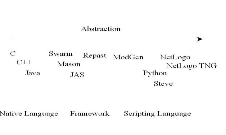
The toolkits described above in addition to the microsimulation models described earlier can be thought of as lying on a continuum. At one end are the microsimulation models written in native code such as C and C++ for example DYNASIM and SAGE. Next, there are
Figure 1. Representation of Agent Based Modelling Methods
It would seem natural to use the most abstract method available in order to gain the maximum assistance from the development platform. However, this must not be at the expense of functionality, flexibility or operating speed of the final model. A platform to model household expenditure should have the following characteristics. These represent factors to be taken into consideration in the selection of modelling environment.
Ease of programming – an efficient well-documented language.
Ease of use – of the platform and completed model.
Size of community – the presence of many users suggests that the platform has wide application and is well supported.
Representation of space – the platform should be capable of showing the relative locations of agents.
Multiple levels - the model should be able to represent agents at the individual, household and regional levels.
File input and output – it will be necessary to read data from a survey such as the FES and write out the results for further analysis.
No limit on the number of agents – survey data often contains 5000 or more cases.
Real and artificial data – it should be possible to load the model with survey data or synthetic data.
Programming language – the platform should support a fully featured programming language.
Graphical plots – this would be a useful feature to monitor parameters while the model was running.
Represent interaction between agents – the behaviour of one agent can affect another.
Alter parameters when running – this would be useful in the simulation of macroeconomic or demographic changes.
Operating speed – the model should run at an acceptable speed, ideally less than a minute to execute one simulated year.
A review of the documentation associated with these platforms showed surprisingly that none of the toolkits appeared to lack the capability to meet the above requirements. Although more detailed investigation by installing each one and testing each function individually might uncover exceptions, the features generally seem to be standard characteristics of agent based modelling toolkits. For this reason it was decided to look in more detail at one of the platforms that allow models to be built using a scripting language. Railsback et. al. ‘strongly recommend NetLogo for prototyping models that may be implemented in lower-level platforms’. Gilbert42 makes extensive use of NetLogo in illustrating a range of social science simulation models. The documentation for NetLogo was found to be excellent and a range of existing models could be run from the NetLogo home page in the form of applets. The ‘patch’ ‘turtle’ format meshes very well with the requirement to simulate households and individuals respectively.
2.3
Household Demand
The next problem for this project to address is to predict the proportion of household budget that will be allocated to a range of goods. This will include ICT items and also competing items such as food, housing and fuel.
2.3.1 Regression Methods
Simple linear regression is a widely used statistical technique for representing the relationship between two parameters or variables. If the variables are plotted on a graph, the regression equation is represented by a straight line drawn such that the variation of the data points above and below the line is minimised. This ‘line of best fit’ is represented by the equation
Y = b0 + b1 X
Y is known as the dependent variable because its value is thought to depend on the value of
X, which is the independent variable. b0 and b1 are constants. For this approach to be valid,
the data should lie close to the straight line and the errors should be normally distributed with a mean of zero. However, the method is robust to small departures from these conditions. Multiple linear regression is an extension of simple linear regression to include more than one independent variable. In this case, the equation takes the form
Y = b0 + b1X1 + b2X2 + b3 X3
modelling household expenditure however it does have limitations. Estimating separate demand equations for each commodity ignores any interaction between them. This can result in biased and distorted results.
2.3.2 Demand Systems
To alleviate this problem, a range of demand systems has been developed specifically for the purpose of econometric analysis and some of these have been applied successfully at Chimera. These are based on the idea of a rational consumer with income y to spend on n types of product, Q = (Q1, …, Qn) with prices p = (p1, …, pn). Income y and prices p are assumed to be
exogenous or independent. The consumer chooses a combination of goods q = (q1, …, qn)
attainable within income y such that y = p q where utility u(q) is maximised according to the customer’s preferences. Utility is conceived as the desirableness or level of satisfaction that can be gained from possession of the goods.
The first complete demand system was the Linear Expenditure System43. This is derived from the Stone-Geary utility function, u(q) = Π (qi - γi)βi where γi is the minimum subsistence
consumption. It can be shown that utility is maximised when
qi = γi - β (y - Σpj γj) / pi (for i = 1,…,n).
This has subsequently been built upon by the Rotterdam model4445 and the Translog46 model. Budget shares can be obtained in the Rotterdam model by
wi dlogqi = Σθ*ij dlogpj + µi dlogy (i = 1,…,n)
and from the Translog model using the formula
wi = αi + Σβik ln(pi/y) / Σαj + ΣΣβjk ln(pk/y)
Currently, the state of the art in demand system estimation seems to be the Almost Ideal Demand System (AIDS)47 with its variants the Quadratic AIDS48 and the semi-flexible Almost
Ideal Demand System49.
The general model for the Almost Ideal Demand system is specified as: - Wi = αi + γij ln Pj + βi ln [M/P]
Where:
Wi is the budget share of the ith good.
M is the total consumption expenditure. Pj is the price of the jth good.
P is a price aggregator.
Demand systems have been successfully applied in a wide range of applications but the assumption of rationality on the part of the consumer has been questioned from a number of quarters. In Bourdieu’s theory of practice, the individual acts largely according to a system of unconscious dispositions to action called the habitus50 51. Galbraith52 claims that consumers are
manipulated by producers through the medium of advertising. According to Veblen53,
individuals may choose more expensive goods simply because they are more expensive. A behaviour that could play havoc with demand curves if found to be widespread. The effect of assuming rationality on the part of the individual is that it constrains behaviour to make it predictable. A rational agent can do no other than choose the optimum outcome. This makes the problem tractable but it also imposes a narrow view in the interpretation of human
only the homogeneous and symmetric versions of the Rotterdam model should properly be used for modelling the demand behaviour of Spanish consumers. In the current project, the demand model will operate on data generated from the microsimulation. Different scenarios will generate new data and it will not be possible to predict in advance which if any of the demand systems can be used. This could result in the necessity of alternating between for example an AIDS and Rotterdam model between simulation runs.
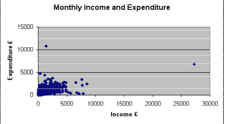
[image:16.595.102.465.206.407.2]Demand systems typically include the assumptions that the consumer spends all of their income on the bundle of goods and cannot spend more than their income. This was asserted in the equation y = p q where income y was equal to the product of the prices and quantities of the selected goods.
[image:16.595.101.465.439.648.2]Figure 1: Relationship between Income and Expenditure
Figure 2: Income and Expenditure for Households with Low Incomes
To test this assumption for Expenditure and Food Survey (EFS) data, I plotted household income (INCANON) from the Expenditure and Food Survey 2006 DVHH against household expenditures (FSALL). If income and expenditure were equal then all points would lie on the same line where the value on the x-axis equals that of the y-axis. As the graphs below show, the data points spread throughout the positive quadrant of the graph. The reasons for this are unclear however it appears to indicate that departures from the assumption of income
£1000 on each axis (Figure 2). It can be seen that for every income level there is a wide variation in expenditure.
Other economic theories such as the Permanent Income Hypothesis55, the Life Cycle
Hypothesis56 and the Relative Income Hypothesis57 allow investigation into this area however the integration of expenditure and income theory remains problematic. One way to integrate income, prices, wealth and demographic variables would be to construct a neural network model. In this case, the variables would be included as input parameters and the network would be trained to associate them with the resulting expenditure pattern from the EFS.
2.3.3 Neural Networks
Artificial neural networks were inspired by the operation of natural brains. Unlike a conventional computer where an item of data has an identifiable location or address, in a neural network, information is distributed throughout the network in the connection strength between a number of cells or neurones. There are many configurations of neural network but a typical one consists of three layers of nodes - an input layer that receives information about the environment, an output layer that indicates the network’s response to the inputs and a hidden layer between them that detects features or patterns in the data. All nodes are linked to those in the adjacent layer by a ‘weight’ that modulates the connection strength between nodes. The weights store whatever information the network obtains from its environment. The neural network is often implemented as a computer program. Once the network structure or topology has been set, it is prepared for a particular application by a process of ‘training’. The weights are initially set at random and training proceeds by repeatedly presenting inputs and outputs to the network. The error for each pattern is calculated and the weights are adjusted in such a way as to reduce the error. Following the training process, the network can
‘recognise’ an input pattern and produce the appropriate response. It can also ‘generalise’ from its knowledge when it encounters input patterns it has not seen before.
A problem that arises from neural networks is that since information is distributed across the network, it is difficult to discover what features of the data it is using to produce a response. Significant research effort has been devoted to this area in recent years. Gerolimetto et.al.58 report the calculation of elasticities and the significance of input parameters in the analysis of wine demand in Italy.
Neural networks can represent non-linear relationships and they are robust to noisy or
3
A prototype model
In order to test the approaches described above and to evaluate the value of Netlogo as a tool, a prototype simulation was implemented in two phases. First, demographic processes are modelled to advance the population over time. Second, the demand expected from the new population is estimated.
3.1
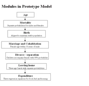
Demographic Processes
Ageing - For each year and for each household and for each simulated resident - Age is increased by 1 year.
Mortality - Test whether the agent dies before the end of the year. For males aged 40 and younger the probability of not surviving p = 0.000736. For males over 40, p = 0.00003 e^0.0954 age. For females 40 and younger p = 0.000411 for females over 40 p = 0.00001 e^0.1017 age. Source: ONS life tables under 40s is an average over 40s fitted with an exponential function.
Birth - Decide when to create new agents. Mothers must be aged from 16 to 43.5. The probability of a birth in any year is 0.1 this was chosen to be just enough to replace the population. The birth rate is the same for single and co-habiting agents.
Marriage - Set up new households first, non-married males aged 16 and over check that there are any eligible females ie. age 16 and over and aged within 10 years of
themselves. If there are any then with a probability depending on the age of the agent they move to a vacant patch and move a female to that patch as well.
Divorce - Marriages end with a probability of 0.0118 per year. This was estimated from the value of 11.8 per thousand in ‘Demographic Trends in the UK’, by Finch 2001. The same procedure with the same probabilities is used for cohabitation. More accurate probability estimates will be derived from the BHPS or existing microsimulation models.
Leaving home - Agents are able to leave home to live on their own. They leave with a probability of 0.01 in a particular year. This is estimated to bring about an average household size of close to the current value of 2.3.
After the demographic phase, expenditure is estimated from an equation obtained by linear regression using data from the BHPS.
Figure 3: Module execution order
3.2
User interface
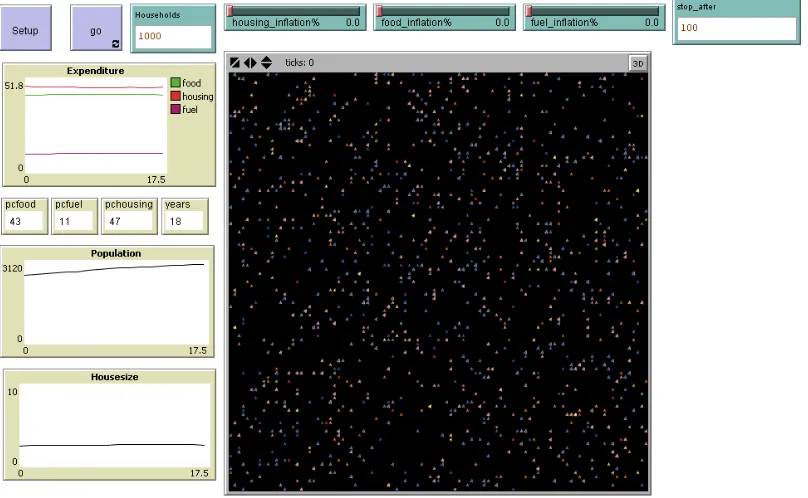
Figure 5: User Interface for Prototype Microsimulation
Agents are represented on the large grid and can be colour coded to indicate information such as whether the agent is single / married or male / female. Initial values for the number of households can be set from the ‘Households’ input box, as can the number of years for the simulation to run in the ‘stop_after’ box. The current population and household size are indicated on graphs which update while the simulation is running. The budget share of food, housing and fuel is shown graphically as well a numerically. The inflation rate for each commodity can be adjusted while the program is running using the sliders. When the ‘setup’ button is pressed, the base data is loaded to initialise the agents. The simulation is initiated by pressing the ‘go’ button.
The model has been converted to a java applet and can be used online - http://istr.essex.ac.uk/tasc/students/tlawso/model1/
3.3
Validation
Figure 4: Validation of sex ratio
4
Summary
This literature review has critically assessed previous research in the areas of microsimulation, agent based modelling, demand systems and neural networks. It reviewed a range of agent-based modelling toolkits and presented a prototype instance of the use of Netlogo to build a dynamic household microsimulation model.
5
Bibliography
1 Seetharamdoo, J. (2006) What if the consumer stops spending, Group Economics, Royal
Bank of Scotland. Retrieved from
http://www.rbs.com/content/economic/downloads/insight/US_consumer.pdf
2 De Agostini, P., and Anderson, B., (2005) WMM D3.3 ‘Utilities’ trends, elasticities and cohort analyses. Ipswich: Chimera, University of Essex.
3 Zong, P. and Anderson, B. (2006) Modelling and forecasting UK telecommunications
expenditure using household microdata, Chimera Working Paper 2006-14, Ipswich:
University of Essex.
4 Armstrong, J. S. (ed.) (2001) Principles of Forecasting, A Handbook for Researchers and Practitioners, Springer, New York.
5 Harding, A. (ed.) (1996) Microsimulation and Public Policy, Amsterdam, North Holland.
6 Sutherland, H., Taylor, R. and Gomulka, J. (2002) ‘Combining Household Income and
Expenditure Data in Policy Simulations’, Review of Income and Wealth, Series 48, Number 4, December 2002.
7 Deaton, A. S. and Muellbaeur, J. (1980) ‘An Almost Ideal Demand System.’ American
Economic Review 70:3 (June): 312-326.
8 Christensen, L., Jorgenson, D. and Lawrence, L. (1975): ‘Transcendental Logarithmic Utility
Functions’, The American Economic Review, 65, 367-383.
9 Barten, A. (1964) ‘Consumer Demand Functions under Conditions of Almost Additive
Preferences’, Econometrica, 32, 1-38.
10 Theil, H. (1965) ‘The Information Approach to Demand Analysis’, Econometrica, 33, 67-87.
11 Orcutt, G. H. (1957) ‘A new type of socio-economic system’ Review of Economics and Statistics, 39(2), 116-123. Reprinted in the International Journal of Microsimulation
(2006) 1(1), 2-8.
12 Orcutt, G., Greenberger, M., Korbel, J. and Wertheimer, R. 1961, Microanalysis of
Socioeconomic Systems: A Simulation Study, Harper and Row, New York.
13 Orcutt, G., Caldwell, S., Wertheimer, R., Franklin, S., Hendricks, G., Peabody, G., Smith, J.
and Zedlewski, S. 1976, Policy Exploration through Microanalytic Simulation, The Urban Institute, Washington DC.
14 Favreault, M. and Smith, K. (2004) A Primer on the Dynamic Simulation of Income Model
(DYNASIM3), The Urban Institure, retrieved from
http://www.urban.org/uploadedpdf/410961_Dynasim3Primer.pdf
15 U.S. Census Bureau (2006) Survey of Income and Program Participation, retrieved from
16 Zayatz, T. (1999) “Social Security Disability Insurance Program Worker Experience.”
Actuarial Study No. 114. Baltimore: Office of the Chief Actuary of the Social Security Administration.
17 Zaidi, A. and Rake, K. (2001) “Dynamic Microsimulation Models: A Review and Some
Lessons for SAGE”, SAGE Discussion Paper no. 2, SAGEDP/02. Retrieved from http://www.lse.ac.uk/collections/SAGE/pdf/SAGE_DP2.pdf
18 Society of Actuaries (2007) Chapter 5 Corsim, Schaumburg, IL, USA, Table 5-1. Retrieved
from http://www.soa.org/files/pdf/Chapter_5.pdf
19 Morrison, M., Dussault, B. (2000) “Overview of Dynacan: a full-fledged Canadian actuarial
stochastic model designed for the fiscal and policy analysis of social security schemes”, IAA Website. retrieved from
http://www.actuaires.org/CTTEES_SOCSEC/Documents/dynacan.pdf
20 Zaidi, A. and Rake, K. (2001) op cit.
21 ibid.
22 ibid.
23 ibid.
24 Hills, J. (2006) ‘From Beveridge to Turner: Demography, Distribution and the Future of
Pensions in the UK’, Centre for Analysis of Social Exclusion, London School of Economics. retrieved from http://sticerd.lse.ac.uk/dps/case/cp/CASEpaper110.pdf
25 Cheesbrough, S. and Scott, A. (2003) ‘Simulating Demographic Events in the SAGE Model’, SAGE Technical Note no. 4, SAGE.
26 Scott, A. (2003) ‘Implementation of demographic transitions in the SAGE Model’, SAGE Technical Note no. 5, SAGE.
27 Harding, A. (2007) ‘Challenges and Opportunities of Dynamic Microsimulation Modelling’,
NATSEM, University of Canberra.
28 ibid P. 5.
29 von Neumann, John (1966). in A. Burks: The Theory of Self-reproducing Automata. Urbana,
IL: Univ. of Illinois Press.
30 Turing. A. (1937), "On Computable Numbers, With an Application to the
Entscheidungsproblem", Proceedings of the London Mathematical Society, Series 2, Volume 42 (1936-37) pp230-265.
31 Gardner, Martin (October 1970), "Mathematical Games: The fantastic combinations of John
Conway's new solitaire game "Life"", Scientific American223: 120–123 .
33 Reynolds, C. (2008) Boids: Background and Update. http://www.red3d.com/cwr/boids/
34 Swarm Development Group http://www.swarm.org/index.php?title=Main_Page
35 Repast, Recursive Porous Agent Simulation Toolkit, http://repast.sourceforge.net/
36 MASON, Multi Agent Simulator of Networks http://cs.gmu.edu/~eclab/projects/mason/
37 Java Agent-based Simulation Library http://jaslibrary.sourceforge.net/index.html
38 Wilensky, U. (1999) NetLogo http://ccl.northwestern.edu/netlogo/
39 Tobias, R. and Hoffmann, C. (2004) ‘Evaluation of free Java-libraries for social-scientific
agent based simulation.’, Journal of Artificial Societies and Social Simulation, 2004;7. retrieved from http://jasss.soc.surrey.ac.uk/7/1/6.html
40 Railsback, S. F., Lytinen, S. L., Jackson, S. K. (2006) ‘Agent-based Simulation Platforms:
Review and Development Recommendations’, Simulation, Vol. 82, No. 9, 609-623.
41 Sonnessa, M. (2004) User’s Guide, JAS Library, Version 1.0.
http://jaslibrary.sourceforge.net/files/UserGuide.pdf
42 Gilbert, N. and Troitzsch, K. G. (2005) ‘Simulation for the Social Scientist – second edition’,
Open University Press, England.
43 Stone, R. (1954) ‘Linear Expenditure System and Demand Analysis: an Application to the
Pattern of British Demand’, The Economic Journal, 64, 511-527.
44 Barten, A. (1964) ‘Consumer Demand Functions under Conditions of Almost Additive
Preferences’, Econometrica, 32, 1-38.
45 Theil, H. (1965) ‘The Information Approach to Demand Analysis’, Econometrica, 33, 67-87.
46 Christensen, L., Jorgenson, D. and Lawrence, L. (1975) ‘Transcendental Logarithmic Utility
Functions’, The American Economic Review, 65, 367-383.
47 Deaton, A. S. and Muellbaeur, J. (1980) op cit.
48 Banks J., Blundell R., Lewbel, A., (1997) Quadratic Engel Curves and Consumer Demand,
Review of Economics and Statistics 79, 527-539.
49 Moschini, G. (1998) The semi-flexible Almost ideal Demand System, European Economics
Research 42: 349-364.
50 Bourdieu, P. (1977) engl. Outline of a Theory of Practice, Cambridge University Press.
51 Bourdieu, P. (1984) engl. Distinction: a Social Critique of the Judgment of Taste, translated
by Richard Nice, Harvard University Press.
53 Veblen, Thorstein. (1899) Theory of the Leisure Class: An Economic Study in the Evolution of Institutions. New York: Macmillan.
54 Molina, J. A, (2002) ‘Modelling the Demand Behaviour of Spanish Consumers Using
Parametric and Non-parametric Approaches’, Studies in Economics and Econometrics, 26(2).
55 Friedman, M. (1957) A Theory of the Consumption Function, National Bureau of Economic
Research Princeton, N.J.
56 Hall, R. E. (1979) Stochastic Implications of the Life Cycle-Permanent Income Hypothesis:
Theory and Evidence, NBER.
57 Duesenberry, J. S. (1949) Income, Saving and the Theory of Consumer Behaviour,
Cambridge, Mass.
58 Gerolimetto, M., Mauracher, I. and Procidano, I., (2005) ‘Analysing Wine Demand with
Artificial Neural Networks’, Presentation to the 11th Congress of the EAAE, Retrieved from