Rhythmic auditory cortex activity at multiple timescales shapes stimulus–response gain and background firing

Systems/Circuits

Rhythmic Auditory Cortex Activity at Multiple Timescales

Shapes Stimulus–Response Gain and Background Firing

Christoph Kayser,

_{Caroline Wilson,}

_X

_{Houman Safaai,}

_{Shuzo Sakata,}

_{* and Stefano Panzeri}

_*

1_{Institute of Neuroscience and Psychology, University of Glasgow, Glasgow, G12 8QB,}2_{Strathclyde Institute of Pharmacy and Biomedical Sciences,}

University of Strathclyde, Glasgow, G1 1XQ, United Kingdom, and3_{Neural Computation Laboratory, Center for Neuroscience and Cognitive Systems,}

Istituto Italiano di Tecnologia, I-38068 Rovereto, Italy

The phase of low-frequency network activity in the auditory cortex captures changes in neural excitability, entrains to the temporal structure of natural sounds, and correlates with the perceptual performance in acoustic tasks. Although these observations suggest a causal link between network rhythms and perception, it remains unknown how precisely they affect the processes by which neural populations encode sounds. We addressed this question by analyzing neural responses in the auditory cortex of anesthetized rats using stimulus–response models. These models included a parametric dependence on the phase of local field potential rhythms in both stimulus-unrelated background activity and the stimulus–response transfer function. We found that phase-dependent models better reproduced the observed responses than static models, during both stimulation with a series of natural sounds and epochs of silence. This was attributable to two factors: (1) phase-dependent variations in background firing (most prominent for delta; 1– 4 Hz); and (2) modulations of response gain that rhythmically amplify and attenuate the responses at specific phases of the rhythm (prominent for frequencies between 2 and 12 Hz). These results provide a quantitative characterization of how slow auditory cortical rhythms shape sound encoding and suggest a differential contribution of network activity at different timescales. In addition, they highlight a putative mechanism that may implement the selective amplification of appropriately timed sound tokens relative to the phase of rhythmic auditory cortex activity.

Key words: delta rhythm; information coding; LNP models; network state; neural coding; receptive fields

Introduction

Accumulating evidence suggests that low-frequency rhythms play an important role for hearing (Schroeder and Lakatos, 2009; Giraud and Poeppel, 2012;Leong and Goswami, 2014). Neuro-imaging and intracranial recordings show that neural activity in the auditory cortex (A1) at frequencies below⬃12 Hz entrains to the temporal structure of sounds and carries information about

sound identity (Kayser et al., 2009;Szymanski et al., 2011;Ding and Simon, 2012,2013;Ng et al., 2013), possibly because natural sounds contain important acoustic structures at these frequen-cies (Ding and Simon, 2013;Doelling et al., 2014;Gross et al., 2013). Importantly, the degree of rhythmic entrainment corre-lates with perceptual intelligibility (Mesgarani and Chang, 2012; Doelling et al., 2014;Peelle et al., 2013), linking the timescales relevant for acoustic comprehension with those of neural activity (Rosen, 1992;Ghitza and Greenberg, 2009;Zion Golumbic et al., 2012). Based on these results, it has been hypothesized that slow rhythmic activity in the A1 reflects key mechanisms of sound encoding that have direct consequences for hearing (Giraud and Poeppel, 2012;Peelle and Davis, 2012;Strauß et al., 2014b).

This raises the central question of how precisely rhythmic auditory cortical activity shapes sensory information processing. Electrophysiological recordings showed that slow rhythms reflect fluctuations in cortical excitability (Bishop, 1933; Azouz and Gray, 1999;Womelsdorf et al., 2014;Pachitariu et al., 2015;Reig et al., 2015) and the strength of neuronal firing (Lakatos et al., 2005;Belitski et al., 2008;Haegens et al., 2011). Such intrinsic excitability changes could either simply reflect stimulus-unrelated modulations of background firing or could reflect a profound influence of cortical dynamics on the sensory computations by individual neurons. Indeed, a prominent theory suggests that auditory network rhythms help to selectively amplify the en-coding of acoustic inputs that are aligned appropriately with the phases of network excitability captured by these rhythms

Received Jan. 21, 2015; revised March 17, 2015; accepted April 7, 2015.

Author contributions: C.K., S.S., and S.P. designed research; C.K., C.W., and H.S. performed research; C.K., C.W., S.S., and S.P. contributed unpublished reagents/analytic tools; C.K., H.S., and S.P. analyzed data; C.K., S.S., and S.P. wrote the paper.

The initial stages of this work were supported by the Max Planck Society (C.K.) and were part of the research program of the Bernstein Center for Computational Neuroscience (Tu¨bingen, Germany) funded by the German Federal Ministry of Education and Research (FKZ 01GQ1002; C.K. and S.P.). The work was also supported by the Action on Hearing Loss (“Flexi Grant”; to C.K.), Medical Research Council Grant MR/J004448/1 (to S.S.), the SI-CODE Project of the FP7 of the European Commission (FET-Open, Grant FP7-284553; to S.P.), and the Autonomous Prov-ince of Trento (“Grandi Progetti 2012,” the “Characterizing and Improving Brain Mechanisms of Attention–ATTEND” project; to S.P.). We are grateful to N. K. Logothetis and R. Brasselet for collaborations in previous phases of this work.

*S.S. and S.P. contributed equally to this work. The authors declare no competing financial interests.

This article is freely available online through theJ NeurosciAuthor Open Choice option.

Correspondence should be addressed to C. Kayser, Institute of Neuroscience and Psychology, University of Glas-gow, 58 Hillhead Street, Glasgow G12 8QB, UK. E-mail:[email protected].

C. Wilson’s present address: Medical Research Council Institute of Hearing Research Nottingham, University of Nottingham, University Park Nottingham, NG7 2RD, UK.

DOI:10.1523/JNEUROSCI.0268-15.2015 Copyright © 2015 Kayser et al.

(Schroeder and Lakatos, 2009;Lakatos et al., 2013). However, whether and how precisely network activity affects the com-putations by which auditory neurons represent sensory inputs remains unknown.

To directly investigate this relationship, we recorded spiking activity and local field potentials (LFPs) in the rat primary audi-tory cortex (A1) during acoustic stimulation and epochs of si-lence. We developed linear–nonlinear Poisson (LNP) models that included, besides a static stimulus–response tuning [spectro-temporal receptive fields (STRFs)], parameters for sensory gain and stimulus-unrelated background activity that varied with the state of network activity as indexed by the phase or power of LFPs at different timescales. Using these models, we uncovered that including a systematic dependence on LFP phase of both back-ground activity (prominent for delta, 1– 4 Hz) and of stimulus– response gain (prominent between 2 and 12 Hz) improved response prediction. These results highlight mechanisms by which systematic changes in stimulus–response transfer could selectively amplify or attenuate responses at specific phases of network rhythms and provide a possible neural underpinning for rhythmic sensory selection and perception (Vanrullen et al., 2011;Giraud and Poeppel, 2012;Jensen et al., 2012).

Materials and Methods

General procedures and data acquisition.Recordings were obtained from six adult Sprague Dawley rats (males, 253–328 g). Experiments were performed in accordance with the United Kingdom Animals (Scientific Procedures) Act of 1986 and were approved by the United Kingdom Home Office and the Ethical Committee of Strathclyde University. The general procedures followed those used in previous work (Sakata and Harris, 2009). The animals were anesthetized with 1.5 g/kg urethane, and lidocaine (2%, 0.1– 0.3 mg) was administered subcutaneously near the site of incision. Body temperature was maintained at 37°C using a feed-back temperature controller. To facilitate acoustic stimulation, a head post was fixed to the frontal bone using bone screws, and the animal was placed in a custom head restraint that left the ears unobstructed. Record-ings took place in a single-walled soundproof box (MAC-3l IAC Acous-tics). After reflecting the left temporalis muscle, the bone over the left A1 was removed and a small duratomy was performed. A 32-channel silicon tetrode probe (A8x1-tet-2mm-200-121-A32; NeuroNexus Technolo-gies) was inserted slowly (⬍2␮m/s) into infragranular layers of A1 using a motorized manipulator (DMA-1511; Narishige). During recording, the brain was covered with 1% agar/0.1MPBS to reduce pulsation and to keep the cortical surface moisturized. Recordings started after a waiting period of⬃30 min. Broadband signals (0.07 Hz to 8 kHz) were amplified (1000 times) using a Plexon system (HST/32V-G20 and PBX3) relative to a cerebellar bone screw and were digitized at 20 kHz (PXI; National Instruments).

Acoustic stimuli were generated through a multi-function data acqui-sition board (NI-PCI-6221; National Instruments) and were presented at a sampling rate of 96 kHz using a speaker driver (ED1; Tucker-Davis Technologies) and using free-field speakers (ES1; Tucker-Davis Tech-nologies) located⬃10 cm in front of the animal. Sound presentation was calibrated using a pressure microphone (PS9200KIT-1/4; ACO Pacific) to ensure linear transfer and calibrated intensity. For this study, a series of naturalistic sounds was presented. These sounds were obtained from previous work (Kayser et al., 2009) and reflect various naturalistic noises or animal calls that were recorded originally in the spectral range of 200 Hz to⬃15 kHz. For this study, they were shifted into the rat’s hearing range by resampling to cover frequencies up to⬃30 kHz (for a spectral representation, seeFig. 1A). The stimulus sequence lasted 30 s and was presented at an average intensity of 65 dB rms and was repeated usually 50 times during each experiment with an interstimulus interval of up to 5 s. We also recorded spontaneous activity before the sound presentation for a period of 250 s.

Neural signals were processed as follows. Spike detection for each tetrode took place offline and was performed with freely available software (EToS

version 3;http://etos.sourceforge.net; Klusters,http://klusters.sourceforge.net;

Hazan et al., 2006;Takekawa et al., 2010), using exactly the standard parameters described in previous studies (Takekawa et al., 2010). Broad-band signals were high-pass filtered, spikes were detected by amplitude thresholding, and potential artifacts were removed by visual inspection. We recorded reliable spiking activity fromn⫽38 sites (of 48 sites in total) and analyzed this as multiunit activity (MUA). We also performed clustering with the Klusters software and isolated single units based on a spike isolation distance of⬎20 (Schmitzer-Torbert et al., 2005). How-ever, the overall spike rate of single units in this preparation was low (mean response during stimulation of 1.9⫾0.3 spikes/s; mean⫾SEM across units) and hence did not allow us to perform on the LFP-dependent analysis described below on single-unit activity because of undersampling of the response space. Hence, we restrict the present re-port to MUA data.

For every recording site, field potentials were extracted from the broad-band signal after resampling the original data to 1000 Hz sample rate and were averaged across all four channels per tetrode. A Kaiser finite impulse response filter (sharp transition bandwidth of 1 Hz, pass-band ripple of 0.01 dB, and stop-band attenuation of 50 dB; forward and backward filtering) was used to derive band-limited signals in different frequency bands (for details, seeKayser, 2009). Here we focused on the following overlapping bands, [0.25–1], [0.5–2] and [1– 4] Hz and con-tinuing in 4-Hz-wide bands up to 24 Hz. The instantaneous power and phase of each band was obtained from the Hilbert transform. To relate spike rates and stimulus encoding to the phase or power of each band-limited signal, we labeled each spike with the respective parameter re-corded from the same electrode at the time of that spike (Kayser et al., 2009). For phase, this was achieved by using equally spaced bins covering the 2␲cycle. For power, we divided the range of power values observed on each electrode into equally populated bins. For the results reported here, we used four bins, but using a higher number (e.g., eight bins) did not change the results qualitatively. We focused on frequencies⬍24 Hz because preliminary tests had revealed that modulations of firing rates were strongest at low frequencies.

Terminology and assessment of cortical states.The term cortical state is used in the literature to describe a wide range of phenomena, with intrin-sically different timescales, but usually varying on the scale of hundreds of milliseconds or longer (Curto et al., 2009;Harris and Thiele, 2011;

Marguet and Harris, 2011;Sakata and Harris, 2012;Pachitariu et al., 2015). An example is a transition between the synchronized or desynchro-nized (also up/down) states. These slow and relatively widespread net-work state transitions are likely different from the more rapid changes in network excitability indexed by the phase or power of LFP bands⬎0.5 Hz (Canolty and Knight, 2010;Panzeri et al., 2010;Haegens et al., 2011;

Lakatos et al., 2013). To distinguish these two timescales of network properties, here we use the term “cortical state” for properties of network dynamics on scales of seconds or longer (such as the synchronized and desynchronized states that can be detected from the LFP spectrum) and use the term LFP state to denote cortical dynamics indexed by the power or phase of different LFP bands, which persist on shorter timescales. This nomenclature is conceptually similar to that ofCurto et al. (2009), who distinguished between “dynamic states” of cortex referring to properties of network dynamics on a timescale of seconds or more and “activity states” describing cortical states that persist on shorter timescales of few tens to few hundred milliseconds.

We quantified cortical state using the ratio of low-frequency (0.25–5 Hz) LFP power divided by the total LFP power (0.25–50 Hz) and using the correlation of firing rates across distant electrodes (Curto et al., 2009;

Sakata and Harris, 2012;Pachitariu et al., 2015). These measures were correlated across sessions and times, and, when plotted over the experi-mental time axis, they both indicated that cortical states were stable for all but one of six experiments (Experiment 1), during which we observed more pronounced variations in LFP power ratio than for the others (see

across sessions did not confound with our results pertaining to the more rapid network dynamics indexed by LFP phase.

Quantification of LFP state-dependent firing rates and circular phase statistics.To quantify the relation between spikes and LFP phase (or power), we calculated the percentage of spikes elicited in each phase (or power) bin. The “firing rate modulation” with phase was calculated as the firing rate in the preferred bin (i.e., the bin with maximal rate) minus that in the opposing bin (i.e., the bin 180° apart). Using the difference be-tween maximal and minimal firing rate across bins (Montemurro et al., 2008) yielded results very similar to those presented here. For power, the rate modulation was defined as the value in the highest power bin minus that in the lowest. We defined the “preferred phase” for each unit as the circular average of the phase at all spikes. Statistical tests for the non-uniformity of the spike-phase distribution were computed with the Ray-leigh’s test for non-uniformity of circular data.

STRFs and response models.To model the neural input– output func-tion, we used LNP models, schematized inFigure 2A. These models are made of a linear filter characterizing the selectivity of each unit in time and sound-frequency domains (the STRF) and of a nonlinear stimulus– response transfer function translating the stimulus filter activation into a corresponding spike rate (Fig. 2A). We extended this basic model to describe the time-dependent spike rateq(t) as the sum of a stimulus-induced componentqstim(t) plus an additive componentbthat models the presence of ongoing and stimulus-unrelated background firing.

In more detail, for each unit, the STRF was obtained using regularized regression based on the data recorded during stimulus presentation ( Ma-chens et al., 2004;David et al., 2007) and by correcting for the temporal autocorrelation inherent to natural sounds (Theunissen et al., 2001). A time–frequency representation of the stimulus was obtained by resam-pling sounds at 90 kHz and deriving a time–frequency representation using sliding window Fourier analysis (the spectrogram function in MATLAB) based on 100 ms time windows, at 5 ms nominal temporal resolution and by selecting logarithmically spaced frequencies (eight steps per octave) between 800 Hz and 43 kHz. The square root of the power-spectral density was used for the STRF analysis. STRFs were cal-culated based on single-trial responses using ridge regression, introduc-ing two additional constraint parameters for filter smoothness and sparseness (for details, seeMachens et al., 2004). For each neuron, the model parameters (constraints and STRF filter) were optimized using

four-fold cross-validation; that is, we first estimated the STRF filter using three-fourths of the data, and we then computed its performance in predicting responses on the remaining one-fourth. The constraint pa-rameters were optimized within a range of values determined from pilot studies and by selecting the parameter yielding the best cross-validated response prediction. The stimulus-induced firing rate predicted by the LNP model was then completed by adding a static nonlinearity, i.e., a functionu(.) that converts the linear filter output into the stimulus-induced component of the modeled firing rate:

qstim(t)⫽u(STRF(t)⫻Stimulus(t)).

Practically, we estimatedu(.) to calibrate the predicted responseq(t) to the actually observed response. In concordance with previous work ( Ra-binowitz et al., 2011;Zhou et al., 2014), we found that these nonlineari-ties exhibited the typical monotonic increase in spike rate with sensory drive known for cortical neurons (Fig. 3). Hence, we parameterized the nonlinearity using a threshold-linear function (Atencio et al., 2008;

Sharpee et al., 2008):

u共x兲⫽G⫻关x兴_⫹, with [x]_⫹⫽xifx ⬍ 0,关x兴_⫹⫽0 ifx ⱕ 0,

where the parameterGis the stimulus–response gain applied to the lin-early modeled stimulus drive. The prediction of the time-dependent fir-ing rateq(t) of the model was then obtained by adding a parameterbthat accounts for stimulus-unrelated activity:

q共t兲⫽qstim(t)⫹b.

The parametersGandbproviding the best response prediction for each unit were derived using multidimensional unconstrained nonlinear min-imization (fminsearch in MATLAB), as described below. The predictive power of the model was defined as the percentage of explained variance (r2_{), averaged over cross-validation runs.}

We also tested whether a more elaborate nonlinearity based on two parameters (of the formu(x)⫽G⫻[x⫺T]_⫹, with an additional thresh-oldTapplied before rectification) would allow a better response prediction than the one-parameter model above. However, we found that both models explained similar proportions of the response variance across units (r2_⫽ 0.176⫾0.012 and 0.175⫾0.013; mean⫾SEM). The Akaike weights (see

A

5 10 15 20 25 30

0 0 10

20

30

40

Time [s]

Frequency [kHz]

B

0.25

4

8

12

16

20

0 0.5 1 1.5 2 2.5 3

40 10

% Spikes/bin

Spontaneous Stimulus

T

rials

T

rials

Frequency [Hz]

C

Phase bin

0 40

20 60

% Spikes / bin

1st 2nd 3rd 4th

D

1st 2nd 3rd 4th

Time [s]

1-4Hz

Spontaneous

Stimulus

Phase bin

1

0 30 60

% Rate Modulation

Phase bin

below) between these models did not provide strong evidence for either model (0.57⫾0.07 and 0.42⫾0.07), and, for simplicity, we restricted our analysis to the nonlinearity described by Equation 2.

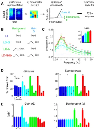
LFP state-dependent models and model comparison.Our goal was to study how current LFP state (denoted␪), indexed by the phase or power of a single LFP band or pairs of bands, influenced the stimulus–response transfer. To this end, we introduced four LNP models that differed in how they include a possible LFP dependency in their model parametersb andG(see Eqs. 2 and 3). All models were fitted using cross-validation to the merged neural responses obtained during stimulus presentation (50 repeats of the 30 s sequence) and silence (250 s of continuous recording). First, we considered an LFP-independent (LI) model, defined by fixed gain and background parameters [b,G], i.e., parameters that are constant

during the entire period of spontaneous activ-ity and acoustic stimulation. This corresponds to typical LNP models computed in previous work (Atencio et al., 2008;Sharpee et al., 2008), except that we fit the model to the combined response obtained during acoustic stimulation and spontaneous activity.

Second, we considered three LFP-dependent models. The parameters of these models [e.g., G(␪)] were allowed to take four different val-ues, one for each binned value of the LFP state (e.g., delta phase): (1) in the LFP-dependent background (LD-b) model [b(␪),G], the offset was allowed to vary with␪, but the gain was fixed; (2) in the LFP-dependent gain (LD-G) model [b,G(␪)], gain varied with␪ but the background was fixed; and (3) in the LFP-dependent gain and background (LD-G&b) model [O(␪),G(␪)], both parameters varied with␪. Note that the number of free parame-ters varied across models (for single LFP bands: LI, two parameters; LD-G and LD-b, five pa-rameters; LD-G&b, eight parameters).

Finally, as a control condition, we also con-sidered an LFP-dependent model without a stimulus-driven component (i.e., Eq. 3 with qstim⫽0 at all times). This model only relied on the variation of background activity to explain the data. This model reproduced the observed data very poorly across frequency bands (e.g., r2_{⫽0.05⫾0.01 for delta) and was not} ana-lyzed further.

We compared the performance of each model in explaining the experimentally ob-served responses using the Akaike information criterion (AIC), which is a standard model se-lection technique that compensates for the variable degrees of freedom between models (Akaike, 1974). The AIC quantifies the descrip-tive power of each model based on the log-likelihood of the observed data, penalizing models with larger numbers of parameters, and is defined as AIC⫽2⫻k⫺2⫻ln(L), wherekis the degrees of freedom, andLis the log-likelihood of the data under this model. Given that we analyzed multiple repeats of the stimulus sequence that are unlikely to be statis-tically independent, we used an effective de-grees of freedom; this was defined as the number of time bins during the baseline period plus the number of time bins of one (rather than all) repeat of the stimulus sequence. We computed Akaike weights, which quantify the relative AIC values within a group of models and which facilitate model comparison within a set of proposed models. For each model, these are defined as exp(⫺0.5⫻AIC) divided by the sum of weights for all models within a group (Burnham and Anderson, 2004). An Akaike weight near 1 suggests a high probability that this model minimizes the information lost relative to the actual data com-pared with the other models.

Note that not all units allow a description based on LNP models. Hence, we restricted the analysis to those sites for which the LI model reached anr2 of at least 0.1 (31 of 38 units). Given that we selected sites based on threshold on performance of the LI model, the better response prediction obtained from the LFP-dependent models cannot result from a selection bias.

Throughout text, results are presented as mean⫾SEM across sites, unless stated otherwise. Statistical comparisons are based on pairedt tests, and, when multiple tests are performed between models or time

Sound

frequency

A

×

ii) Linear filter (STRF)

iii) Output nonlinearity

P[.] = response iv) Poisson

spike train

Spike rate

Filter output

0 40

20 60

% Spikes / bin

0.2

0.1 0.3

D

Background, b

Gain, G

LI

LD-b

Background b

Gain G

fixed

LD-G

LD-G&b

B

fixed fixed

Background (b) Gain (G)

E

-dep.

0

data

-dep. fixed

-dep. -dep.

0 0.6

0.4 0.8

0.2

0 5 10

[arb.]

Spontaneous Stimulus

0 40

20 60

0.25 4 8 12 16 20

Frequency [Hz]

1

prediction [r

2]

0.25

0.2 0.35

0.3

0.15

C

Phase bin Phase bin

frequency bands, these were Bonferroni’s corrected for multiple comparisons.

Single-trial stimulus decoding and sensory in-formation.The sensory information carried by the recorded responses and by the responses predicted by the different models was com-puted using a single-trial decoding approach. For this calculation, we used a nearest-neighbor decoder based on the Euclidean dis-tance between the time-binned (10 ms) spike trains observed in individual trials and the trial-averaged spike trains associated with different stimuli, which was shown to work effectively in previous work (Kayser et al., 2010,2012). As “stimuli” for decoding, we considered 55 sections of 250 ms duration selected within the 30 s stim-ulus period. From the resulting decoding matrix, we calculated the mutual information between stimuli and responses using established proce-dures (Quian Quiroga and Panzeri, 2009;Kayser et al., 2010,2012).

To quantify the contribution of spikes dur-ing different LFP phases to the mutual infor-mation, we repeated the decoding procedure for each unit once by including all spikes (de-notedItot) and then by systematically discard-ing spikes durdiscard-ing each LFP phase␪[denoted

Iignore(␪)]. From this, we calculated the relative

information attributed to spikes during each phase as follows:

Irel(␪)⫽共Itot⫺Iignore(␪))/Itot.

The difference betweenItotandIignore(␪) can be interpreted as the amount of information lost when the decoder selectively ignores spikes emitted during a specific phase quadrant, and thus it represents the amount of information uniquely carried by spikes emitted in the neglected phase quadrant. Thus,Irel(␪) can be interpreted as the fraction of the total in-formation in the spike train that is carried uniquely by spikes emitted at a given phase. The normalization byItotis useful to facilitate comparisons across units carrying different amount of total information. Note that this rel-ative information can be negrel-ative and that neg-ative values indicate that removing a specific set of spikes increases the ability to decode in-dividual sensory stimuli. This can happen, for example, when spikes emitted in a given phase

are almost completely stimulus unrelated, and thus removing them fa-cilitates decoding because it effectively removes noise without removing signal. We also computed an index of information modulation with phase, defined as the difference inIrelbetween the phase bin with highest information minus the information in the opposing bin (i.e., 180° apart). To quantify the effect of changes in firing rate with LFP phase on the modulation of information, we performed the following control analysis. For each unit, we equalized the firing rate across phase bins before stim-ulus decoding as follows. We determined the total number of spikes in the phase bin across all time points and determined the minimum across bins. Then we randomly removed spikes occurring during the other phases to match this minimum number. For each unit, we repeated this process 50 times and averaged the resulting information values.

Results

We recorded spiking activity and LFPs from 38 sites in the A1 of six urethane-anesthetized rats using multi-shank silicon tetrodes. Field potentials and spiking responses were recorded both during

silence (spontaneous activity) and during acoustic stimulation with a series of naturalistic sounds (Fig. 1A). As illustrated by example data (Fig. 1B), firing rates were modulated systemat-ically and reliably by the acoustic stimulus. In addition, in-spection of the LFPs showed that low-frequency network activity was entrained reliably to the stimulus, as well during many epochs of the stimulus period (Fig. 1B). This is illustrated in the example ofFigure 1Bby the fact that phase of delta (1– 4 Hz) band is time locked to the stimulus time course reliably across trials. This frequent entrainment of slow network activity during acoustic stimulation is consistent with previous intracranial re-cordings in awake primates and anesthetized rodents (Lakatos et al., 2008;Kayser et al., 2009;Szymanski et al., 2011) and neuro-imaging results in humans (Howard and Poeppel, 2010;Peelle and Davis, 2012;Ding and Simon, 2013;Gross et al., 2013;Henry et al., 2014). Experimental evidence suggests that fluctuations in slow rhythmic cortical activity reflect changes in network

dynam-0 10 20 30

500 ms

B

+20 -300 0.8

20 40 10

[kHz]

Spike rate

Filter output Time [ms]

A

Firing rate [Spk/s]

+

-LI

LD-G

LD-b

LD-G&b

Data

1-4Hz

-+ +

-o d

o

T

rials

...

...

ics and neural excitability (Bishop, 1933;Azouz and Gray, 1999; Harris and Thiele, 2011;Buzsa´ki et al., 2012;Womelsdorf et al., 2014;Pachitariu et al., 2015;Reig et al., 2015). Hence, the pres-ence of stimulus-locked variations in both firing rates and net-work activity raises the question of whether and how the sensory encoding of individual neurons depends on the network dynam-ics captured by LFP activity at different timescales.

Firing rates are modulated by LFP phase

We first considered the dependence of neuronal firing on the instantaneous phase of individual LFP bands (between 0.25 and 24 Hz). To this end, we partitioned the oscillatory cycle into phase quadrants (i.e., four phase bins;Fig. 1C). Consistent with previous results (Lakatos et al., 2005;Montemurro et al., 2008; Kayser et al., 2009;Haegens et al., 2011), we found that firing rates varied systematically with LFP phase. The degree of firing rate modulation was frequency dependent and was strongest for delta (1– 4 Hz;Fig. 1D) during both acoustic stimulation and sponta-neous activity. During acoustic stimulation, the modulation was 44.4⫾1.2% for delta but only 23.3⫾0.95% for lower frequen-cies (0.25– 0.5 Hz), was⬃15% for alpha (8 –12 Hz) and was⬍5% for frequencies ⬎20 Hz. During spontaneous activity, similar values were obtained (delta: 49.4⫾1.9%;⬍5% for frequencies ⬎20 Hz). The distribution of the preferred phase of firing across units was highly non-uniform for each band during both acoustic stimulation and spontaneous activity (Rayleigh’s test,Zvalues⬎ 30 andp⬍10⫺11_{for all bands).}

The dependence of firing rates on LFP phase during silence likely reflects an intrinsic modulation of network excitability emerging from local connectivity, cellular properties, or brain-wide fluctuations in activity (Schaefer et al., 2006; Harris and Thiele, 2011; Harris and Mrsic-Flogel, 2013; Pachitariu et al., 2015;Reig et al., 2015). The dependence of firing rates on LFP phase during sensory stimulation may either only reflect the same modulation of background firing seen during spontaneous activ-ity but may also reflect an additional dependence of the neuronal stimulus tuning properties on the LFP phase. In the following, we disentangle these contributions using a data-driven mod-eling approach.

LFP state-independent response models

To better understand the interaction between the network dy-namics indexed by LFP phase and the sensory input, we exploited the possibility to describe A1 responses using receptive fields and LNP models (Depireux et al., 2001;Escabi and Schreiner, 2002; Machens et al., 2004;Rabinowitz et al., 2011;Sharpee et al., 2011). These models provide a quantitative description of both the neu-ral selectivity to the time–frequency content of the sound and their input– output transformation (output nonlinearity; Fig. 2A). To derive such models, we started from a time–frequency representation of the auditory stimulus (Fig. 2Ai) and derived a linear filter (STRFs;Aii) associated with the response of each unit and a static nonlinearity (Aiii) describing the transformation be-tween filter activation and the observed responses. The simulated response was obtained as Poisson spike train obtained from the transformed filter response (Fig. 2Aiv).

Traditionally, such models are fit with a fixed set of parame-ters to the spike trains recorded over the entire period of stimulus presentation. We call this traditional approach the LI model (Fig. 2B). Such a model reflects the best possible (LNP-based) stimu-lus–response description that ignores the ongoing changes in network activity. Generally, not all units allow a description by STRFs and LNP models (Atencio et al., 2008;Christianson et al.,

2008). For the present data, 31 of 38 sites allowed a (cross-validated) response prediction during the stimulus period ex-ceeding a criterion ofr2 _{⬎0.1. Examples of STRF filters and}

output nonlinearities are shown inFigure 3A. For subsequent analyses, we modeled these output nonlinearities with a threshold-linear function (see Eq. 2; quality of fit,r2_{⫽0.96⫾0.04). The}

model included also a background parameterbdescribing addi-tive and not stimulus-related components of the observed re-sponse. Thus, the model described the neural responses by specifying its STRF (kept fixed in the following analyses) and two other parameters: (1) the output gainGof the nonlinearity; and (2) the background activity parameterb(Fig. 2Aiii). The gain characterizes the steepness of the output transformation, with higher or lower values reflecting relative amplification or attenu-ation, respectively.

Across units, the average response prediction by the LI model wasr2_{⫽0.18⫾0.01 (Fig. 2C, blue). Although the LI model}

allowed a reasonable description of the stimulus-driven response, it could not explain the phase dependence of neural firing. This can be seen inFigure 2D, which displays the dependence of firing rates on delta phase. First, during stimulus presentation, the LI model predicts a relatively flat distribution, with only a modest variation across phase bins (4.9⫾0.5%), which is much weaker than the variation in the actual data (Fig. 2D, left, black circles; 45.0⫾0.9%;t(30)⫽36;p⬍10⫺5). Second, during spontaneous

activity, the LI model (by definition) predicts a constant and phase-independent firing rate (Fig. 2D, right), a result that devi-ates completely from the observed data. Hence, the LI model is insufficient to explain the observed phase dependence of firing rates.

LFP state-dependent response models

We next considered three extended models in which the model parameters (G,b) could take LFP state-dependent values (Fig. 2B). In the LD-b model, the background firing parameterbvaried with LFP state but the gain was fixed. In the LD-G model, the gain was allowed to vary but the background parameter was not. Fi-nally, in the LD-G&b model, both parameters were allowed to vary with LFP state.

The results inFigure 2Cshow that fitting these models relative to LFP phase improved the response prediction considerably. The largest increase in prediction accuracy (r2_{) over the LI model}

occurred for the delta band and reached nearly twice the value obtained with the LI model (0.30⫾0.02 for the LD-G&b model). Smaller but considerable improvements were observed for lower frequencies (e.g., 0.25– 0.5 Hz) and higher-frequency bands (4 – 8 Hz for theta and 8 –12 Hz for alpha). For frequencies⬎16 Hz, the improvement in response prediction by LFP-dependent models was small, suggesting that LFP state defined at frequency above 16 Hz does not affect much how cortical neurons encode sounds.

Delta phase-dependent response models

For the delta band, all LFP-dependent models provided a better response prediction than the LI model. However, the LD-G&b model (r2 _{⫽0.30 ⫾0.02; Fig. 2C, inset) predicted responses}

significantly better than the LD-G (r2_{⫽0.24⫾0.02;t}

(30)⫽9.7,

p⬍10⫺5_{) or LD-b (r}2_{⫽0.29⫾0.02;t}

(30)⫽4.0,p⬍0.001)

data within the considered set of models. In addition, the LD-b model also predicted the response significantly better than the LD-G model (t(30)⫽7.3,p⬍10⫺5; relative Akaike weights

be-tween these models 0.99⫾0.01 for LD-b), although both had the same number of parameters.

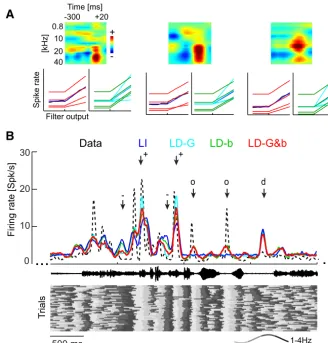
Figure 3illustrates the nature of this improvement in response prediction using example data.Figure 3Aillustrates how the LFP dependence affects the output nonlinearity.Figure 3Bdisplays a section of actual data and predicted responses during acoustic stimulation, shown here as trial-averaged firing rates. The bot-tom ofFigure 3Bdisplays the delta phase on each trial used to compute the LD models. This example illustrates the differences between models and the effect on the predicted responses of both the phase values and their reliable entrainment to the sound. The LI model predicts some of the stimulus-induced response peaks but underestimates response amplitudes, predicts temporally more extended peaks than seen in the actual data, and fails to account for rate changes in periods of low firing. When the LFP phase is entrained to the sound (i.e., phase is consistent across trials), the phase variations in gain and background activity increase (Fig. 3A, marked⫹) or decrease (marked⫺) the firing rate predicted by the LD models compared with the LI model. When the LFP phase is not entrained (marked “d”), all models predict a firing rate because phase has no consistent effect on LD models. Finally, when LFP phase is stimulus entrained but the linear STRF filter predicts no stimulus response (marked “o”), the phase depen-dency of background activity still predicts a reliable variation in firing rate (LD-b and LD-G&b) that coincides with firing varia-tions seen in the actual data. In all, this example demonstrates that accurate prediction of the observed responses requires the correct prediction of periods of stimulus drive by the STRF, the LFP-dependent amplification and attenuation of these, and the pre-diction of responses that are induced by network activity not driven by the stimulus.

A similar picture emerged when comparing how different models predicted how firing rate should vary with delta phase (Fig. 2D). The LD-G model predicted some variation of firing rate with phase during stimulation (21.0⫾0.8%), but these vari-ations were significantly smaller (t(30)⫽31;p⬍10⫺5) than those

observed in the actual data, which were 45.0⫾0.9% (Fig. 2D). By definition, this model predicted that firing rates during sponta-neous activity do not depend on phase and hence failed to ac-count for the observed state dependence during silence, which was 50.5⫾1.7%. The LD-b model predicted a firing rate modu-lation of 43.0⫾0.4% during stimulation, which was closer to the observed data (t(30)⫽3.5,p⬍0.05) than that of the LD-G model.

Moreover, the LD-b model predicted a firing rate modulation during spontaneous activity of 51.9⫾1.3%, which did not differ significantly from that seen during spontaneous activity (t(30)⫽

0.8,p⬎0.05). Finally, the LD-G&b model predicted a firing rate modulation with phase that did not differ from the observed data during both stimulation (45.3⫾0.4%;t(30)⫽1.5,p⬎0.05) and

spontaneous activity (47.2⫾1.1%;t(30)⫽2.6,p⬎0.05).

Phase-dependent sensory gain and background activity To obtain more insights about how the phase dependence of neural responses may affect sensory computations, we report in Figure 2Ethe distributions of the best-fit values of the gain and background parameters. This leads to a better understanding of how the different models describe the neural responses. For ex-ample, the LD-G model necessitates a variation in response gain of a factor of⬃10 across phase bins, a scale that seems unrealis-tically large given reported gain modulations in auditory cortical

neurons (Rabinowitz et al., 2011;Zhou et al., 2014). In contrast, the LD-G&b model not only provides a better response descrip-tion but also features more moderate and credible changes in gain of a factor of⬃2. This lends additional credibility to the LD-G&b model as a better account of the actual data.

The distributions of the best-fit gain and background param-eters also reveal that both paramparam-eters are highest in the first two phase quadrants. These variations in stimulus gain lend them-selves to a simple interpretation of how phase dependence affects neural representations: these gain variations implement a relative amplification of sensory inputs during the first half of the delta cycle and an effective attenuation during the second half. Inter-estingly, gain and background activity vary in a coordinated man-ner, suggesting that both reflect an overall increase of neural excitability during specific epochs of network dynamics. This de-pendence of gain and background on LFP phase has direct implica-tions for the information coding properties of auditory neurons, which we explore next.

Consequences for sensory information encoding

To study the potential effect of state dependence for sensory rep-resentations, we quantified the mutual information between neural responses and the stimulus sequence using single-trial de-coding. We asked whether the above-described modulation by delta phase of the responses of cortical neurons implies that there are privileged phases of the delta cycle that provide a more im-portant contribution to the total information carried by the en-tire spike train than other phase epochs.

To examine the relative information carried by spikes occur-ring at different phases of network rhythms, we computed the relative information carried by each phase bin, defined as the difference between the total information provided by the full response (including all spikes from all phases of the delta cycle) and the information carried after removing all spikes occurring during a specific phase bin, normalized by the total information. This quantity can be interpreted as the fraction of the total infor-mation in the spike train that is uniquely carried by spikes emit-ted at a given phase (see Materials and Methods). Large positive values of this quantity indicate that spikes in the considered phase bin carry crucial unique information, whereas negative values indicate that spikes in that bin carry much more noise than stimulus signal and thus removing them facilitates information decoding.

We first quantified the relative information for different delta band phase quadrants in the actual data. We found (Fig. 4A) that spikes occurring in the first delta quadrant (the one carrying the most relative information) carried approximately six times more information than spikes emitted during the later quadrant carry-ing the least relative information (0.34⫾0.02 vs 0.05⫾0.01; t(30)⫽9.0,p⬍10⫺10;Fig. 4A, black), resulting in an information

modulation of 0.29⫾0.04. Thus, in actual cortical responses, there is a phase-dependent amplification of sensory information at the beginning of the delta cycle compared with later phase epochs. To understand how response gain and background activity contrib-ute to this concentration of information, we compcontrib-uted the infor-mation provided by each model and compared it quantitatively with that of the actual data, using the sum of squares across phase quadrants (SS) as measure of the quality of model fit.

difference in information between phase quadrants can only re-sult from differences in stimulus activation but not changes in network dynamics. The higher firing rates in the first quadrant predicted by the LI model (Fig. 2D) suggest a stronger drive dur-ing the first quadrant, and, indeed, the LI model also predicts more information for spikes in the first compared with later quadrants (Fig. 4A). However, the LI model failed to describe accurately the information in the actual data (SS, 0.19⫾0.03) and resulted in a significantly lower information modulation (0.20⫾0.01; t(30)⫽2.8,p⬍0.01). Hence, phase-dependent

stimulus activation plays a role in shaping the variation in sensory information with delta phase but cannot fully explain it, implying that phase-dependent variations of cortical activity are required to explain the information modulation.

The effect of the state dependence of output gain on informa-tion can be appreciated by comparing the informainforma-tion between the LI and LD-G models. We expected that adding a state-dependent output gain should effectively accentuate the infor-mation carried by spikes in the first quadrants, because these received the strongest gain (Fig. 2). Indeed, the information val-ues from the LD-G model peaked in the first quadrant, and the information modulation was much larger than for the LI model (0.6⫾0.06;t(30)⫽22,p⬍10⫺10;Fig. 4A), demonstrating that

phase variations in gain effectively concentrate the sensory infor-mation during specific epochs of the network cycle. However, the information modulation of the LD-G model was more extreme than that of actual data, and so this model did not provide a significant improvement over the LI model in explaining the ac-tual data (SS, 0.14⫾0.02;Ftest,F⫽1.9,p⬎0.05), suggesting that other factors need to be included to explain the information modulation in the actual data.

Thus, we considered next the effect of background activity on sensory information. This is revealed when comparing the LD-b and SD-G&b models with the LI model. Intuition suggests that adding the phase-dependent background activity should lead to a reduction of information in those phase quadrants where this is highest. Indeed, information values for the LD-b model were highest in the second quadrant, where background activity was weakest (Fig. 2). The LD-b model predicted an informa-tion modulainforma-tion that was comparable with the LI model (0.16 ⫾ 0.01; t(30) ⫽ 1.9, p ⬎ 0.05) but provided a better

approximation to the actual data than the LI model (SS, 0.12⫾ 0.02;F ⫽3.4, p⬍0.01), suggesting that the modulation of

background activity provided by the model plays a part in shaping informa-tion content.

Finally, we considered the combined effect of phase modulation of both gain and background activity, which is cap-tured by the LD-G&b model. This model yielded information values that were much closer to the actual data (SS, 0.07⫾ 0.01). It predicted them significantly bet-ter than the LI (F⫽4.0,p⬍0.01) and all LD (at leastF⫽2.1,p⬍0.05) models and predicted an information modulation that did not differ significantly from the actual data (0.28⫾0.02;t(30)⫽0.25,p⬎

0.05). Together, these findings demon-strate the following: (1) the phase depen-dence of gain effectively concentrates sensory information during the early part of the delta cycle; and (2) the phase depen-dence of background activity moderates this concentration of information at specific epochs, without preventing it.

Given that our previous results demonstrated that phase variations of rate are made of both stimulus-independent and stimulus-dependent components, we hypothesized that phase variations of rate may relate to variations of information in a complex way. In other words, the simultaneous presence of phase variations in stimulus gain and background firing suggest that the observed phase dependence of information could not simply be explained by the phase dependence of rate. To shed light on this issue, we repeated the information analysis after normalizing spike counts across phase quadrants (Fig. 4B). This revealed that, even when accounting for differences in firing rates, there was a considerable residual modulation of information with phase in both the actual data (0.19⫾0.02) and the models (0.19⫾0.02, 0.61⫾0.05, 0.15⫾0.01, and 0.20⫾0.02 for LI, LD-G, LD-b, and LD-G&b, respectively). As for the non-normalized information data inFigure 4A, we found that also for the normalized data the LD-G&b model provided the closest approximation to the infor-mation of the real cortical responses (SS values for LI, LD-G, LD-b, and LD-G&b, respectively: 0.17 ⫾ 0.02, 0.25 ⫾ 0.02, 0.11⫾0.01, and 0.05⫾0.005;Ftests of LD-G&b vs all others, at leastF⫽2.6,p⬍0.05). This shows that increases of firing rates at certain phases cannot be directly interpreted as increases of information, because phase variations in sensory information result from phase-dependent changes in stimulus drive com-bined with changes in the signal-to-noise ratio of sensory rep-resentations induced by variations in sensory gain and background activity. Therefore, to understand how sensory rep-resentations are amplified across the cycle cortical state dynam-ics, it is necessary to separate variations in stimulus-related and stimulus-unrelated components of neural activity, as our models attempt to do.

We repeated the analysis for other frequency bands and found that, similar to the modulation of firing rate, the sen-sory information was most strongly affected by the phase of the delta band. In addition, for all frequency bands, the LD-G&b model provided the best approximation to the observed data, demonstrating that a combination of phase-dependent changes in stimulus-unrelated background activity and sen-sory gain are necessary to explain the data.

A

LI LD-b LD-G Data

0.4

0.2

0 0.6

Rel. information

LD-G&b -0.2

B

0.4

0.2

0 0.6

-0.2

Phase bin Phase bin

All spikes Normalized spike rates

Figure 4. Phase-dependent sensory information.A, Sensory information carried by spikes in each delta phase quadrant, calculated for the actual data (black), and each model. Information is expressed relative to the total information carried by each unit (Irel; see Materials and Methods). For the actual data, spikes in the first phase quadrant carry the most sensory information

Complementary phase dependence exerted by different frequency bands

The results presented above were based on models assuming that both stimulus-related (gain G) and unrelated (backgroundb) contributions depend on the LFP phase at the same frequency. However, it could in principle be that stimulus–response gain and background firing relate to distinct timescales of network activity. Indeed, prominent theories have suggested that different rhythms exert a differential control on stimulus processing ( Lis-man, 2005;Panzeri et al., 2010;Jensen et al., 2012,2014;Bastos et al., 2015), such as the multiplexing of sensory representations and their temporal segmentation in theta and gamma band activity (Lisman, 2005) or the relative contribution of gamma and beta rhythms to feedforward and feedback transmission (Bastos et al., 2015). To test whether this was the case here, we extended the above analysis by now allowing parametersGandbof the LD-G&b model to each dependent on distinct frequency band.

First, we analyzed the phase dependence of firing rates relative to all pairs of frequency bands. This revealed that the firing rate modulation was strongest computed relative to pairs of bands involving the delta band and frequencies between 2 and 12 Hz (Fig. 5A). This suggests that including the LFP dependence rela-tive to multiple bands may indeed improve the predicrela-tive power of stimulus–response models.

Then we repeated the model optimization by varyingGandb with the phase of independent bands. This revealed (Fig. 5B) a strong dependence of response prediction on the band used to optimize the background parameterb, with best predictions oc-curring whenbwas dependent on delta. Varying the band for gain also affected response prediction, although to a smaller de-gree. The best-fitting two-band LD-G&b model was found for the combination ofb(1– 4 Hz) andG(8 –12 Hz) and provided a pre-dictive power ofr2_{⫽0.33⫾0.02. To determine whether this}

two-band model indeed provides a significant predictive benefit compared with any single-band model, we compared the predic-tion of all two-band models to the best-performing single-band model [i.e.,G(1– 4 Hz);b(1– 4 Hz)]. The prediction performance was improved significantly (pairedttests, Bonferroni’s corrected, p⬍0.01) for the combinations ofb(1– 4 Hz) withG(2– 6, 4 – 8, 8 –12, 10 –14 Hz). To determine which combinations of fre-quency bands and models provide the best response prediction of all models considered, we compared the Akaike weights across all combinations of models and pairs of frequency bands (4⫻169 combinations). This revealed that the most likely model was the

combination [b(1– 4 Hz),G(8 –12 Hz)], with an average Akaike weight of 0.31⫾0.08. Models not based on background activity derived from delta or using a response gain based on frequencies outside the range of 2–12 Hz had Akaike weights⬍10⫺5_{. This}

suggests that phase variations in stimulus-unrelated firing and stimulus–response gain relate to distinct timescales of network activity, with variations in background activity being related spe-cifically to the delta band and higher frequencies between 2 and 12 Hz reflecting changes in sensory gain. The parameters of the best two-band model are shown inFigure 5C. These confirm the above result that LFP-dependent models result in rhythmic vari-ations in stimulus-unrelated firing and sensory gain, which (as seen above) result in a concentration of sensory information dur-ing parts of the network cycle.

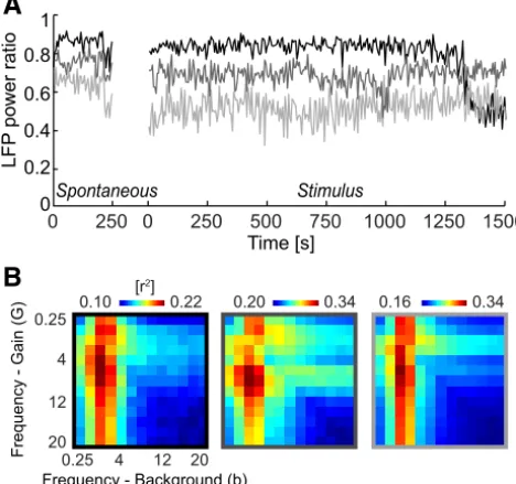
Cortical states and phase-dependent coding

Previous work has shown that neural response properties and the patterns of sensory encoding change with the general state of cortical activity (Curto et al., 2009;Harris and Thiele, 2011; Mar-guet and Harris, 2011;Ecker et al., 2014;Pachitariu et al., 2015). Usually the state of cortical activity is inferred from the ratio between power of low-frequency rhythmic activity (⬍10 Hz) and total power and/or from the pattern of correlations between neu-rons. Prominent low-frequency activity is a sign of a synchro-nized state in which many neurons respond in a coordinated manner (Marguet and Harris, 2011; Sakata and Harris, 2012; Pachitariu et al., 2015). Based on the assessment of the ratio of low-frequency LFP power to the total LFP power, we found that cortical state was mostly stable during our recordings and tended toward the synchronized state (Fig. 6A). Only one of six experi-ments revealed stronger transitions in low-frequency activity over the time course of the recordings (Fig. 6A, black). However, inspection of LD models separately for each experiment showed that the same main result presented inFigure 5Bwas observed consistently across individual experiments and holds regardless of minor changes in cortical state (Fig. 6B).

State dependence relative to the power of network rhythms Given that previous studies have shown that firing rates can be related to the power of LFP bands across a range of frequency bands (Lakatos et al., 2005;Kayser et al., 2009;Haegens et al., 2011), we completed our study by repeating the above analysis using the power rather than the phase of individual LFP bands. This effectively quantifies to which degree changes in LFP power 8

5 _{Rate modulation [%]}

A

Frequency [Hz]

0 0.6

0.4 0.8

0.2

[arb.]

prediction [r

2]

0.18 0.32

B

0.251 4 8 12 16 20

0.25

4

8

12

16

20 1

0.25 1 4 8 12 16 20

0.25

4

8

12

16

20 1

Frequency - Gain (G)

Frequency [Hz] Frequency - Background (b)

Background (b) 1-4Hz Gain (G)

8-12Hz

0 6

4

2

[arb.]

LI LD-G&b

C

Phase bin Phase bin

within a stable cortical state relate to changes in firing rates and LFP-dependent patterns of sensory encoding.

To this end, we divided the range of power values observed on each LFP channel into four equally populated bins. We found that a modulation of firing rate with LFP power was evident for all frequencies tested (Fig. 7A). In general, firing rates were highest when the LFP power was strongest. We then asked whether in-cluding power dependency into the LNP models would provide a similar benefit in response prediction as found for phase. An increase in predictive power relative to the LI model was evident for all LD models for frequency bands⬎1 Hz. However, similar to the firing rate modulation, the predictive power varied little with LFP band (Fig. 7B). In addition, the overall increase in re-sponse prediction was smaller for LFP power than for LFP phase. For example, the best performing single-band model for power [LD-b(8 –12 Hz)] improved response prediction by less than half the amount as obtained by the best single-band model for phase [LD-G&b(1– 4 Hz)]. Importantly, for none of the frequency bands tested did the predictive power of the LD-G&b model excel beyond that of the LD-b model (pairedttests,p⬎0.05). This suggests that the improvement in response prediction by includ-ing state dependence relative to LFP power is primarily explained by changes in stimulus-unrelated background activity and does not relate to changes in sensory gain.

Discussion

We found that response models for A1 neurons yield higher pre-dictive power when including variations in sensory gain and stimulus-unrelated activity relative to the timing (phase) of rhyth-mic network activity. In particular, we found that changes in stimulus-unrelated firing relate to delta phase, whereas changes in sensory gain relate to the phase of frequency bands between 2

and 12 Hz. Our results show that stimulus–response transforma-tions can only be understood when placed in the context of on-going network dynamics and provide a modeling framework to understand such LFP-dependent responses. Second, they suggest a differential effect of auditory cortical network activity at differ-ent timescales on sound encoding. Third, they suggest a neural mechanism by which network rhythms may implement the rhythmic amplification of sound tokens and the rhythmic con-centration of sensory information, a prominent hypothesis put forward previously.

The role of network rhythms for auditory perception

Natural sounds are highly structured at timescales below⬃12 Hz, and this structure is of critical importance for perception (Rosen, 1992;Ghitza and Greenberg, 2009). Combined with the promi-nence of rhythmic activity in the A1 at similar scales (Schroeder and Lakatos, 2009;Ding and Simon, 2013;Doelling et al., 2014; Gross et al., 2013), this has led to the hypothesis that the A1 rhythmically samples the environment at these specific time-scales (Giraud and Poeppel, 2012; Zion Golumbic et al., 2012; Leong and Goswami, 2014).

Support for this hypothesis comes from studies showing that the firing rate of auditory neurons varies with LFP phase (Lakatos et al., 2005;Kayser et al., 2009) and from neuroimaging studies showing that slow cortical rhythms align to acoustic landmarks (Doelling et al., 2014;Gross et al., 2013;Arnal et al., 2014) and are predictive of sound detection or intelligibility (Ng et al., 2012; Peelle and Davis, 2012;Ding and Simon, 2013;Henry et al., 2014; Strauß et al., 2015). However, previous studies did not provide a functional description of the neural computations that may link network rhythms to changes in sound encoding (Giraud and Poeppel, 2012;Poeppel, 2014).

Our results fill this gap and provide a model-driven under-standing of how different network rhythms shape sound encod-ing. First, we found that LI models cannot account for the observed phase dependence of responses. Hence, the correlated stimulus drive to both network rhythms and individual neurons is not sufficient to explain phase-dependent firing rates. Second, we found that purely stimulus-unrelated variations in background activity are also insufficient to explain this phase dependence. Rather, an LFP-dependent output gain is necessary for a more accurate response prediction. Third, our information theoretic analysis shows that a phase-dependent sensory gain effectively leads to an attenuation of sensory inputs during specific epochs of the network cycle and thereby concentrates sensory information in time. This demonstrates that the phase dependence of A1 re-sponses, at least in part, relates to a direct rhythmic modulation of neural sound encoding.

Our results support the hypothesis that the alignment of rhythmic auditory cortical activity to acoustic landmarks helps to selectively amplify those sound tokens that are aligned with the most excitable phase of the network (Schroeder and Lakatos, 2009;Giraud and Poeppel, 2012;Lakatos et al., 2013). Previous work demonstrated a correlation between network dynamics and firing rates, yet this does not necessarily imply a phase dependence of sensory information; any modulation of firing rates could simply result from changes in stimulus-unrelated activity. However, our modeling approach allows disentangling these contributions and shows that LFP phase relates to systematic changes in stimulus– response gain. Hence, LFP-dependent transformations in A1 can indeed serve to selectively amplify the encoding of appropriate timed sound tokens (Lakatos et al., 2013;Arnal et al., 2014).

A

0 250 0 250 500 750 1000 1250 1500

[r2_] 0.10 0.22

0.25 4 12 20 0.25

4

12

20

Frequency - Gain (G)

Frequency - Background (b) Spontaneous

Time [s] 1

0 Stimulus

0.2

0.20 0.34 0.16 0.34

LFP

power ratio

B

0.4 0.6 0.8

Multiple rhythms shape neural responses in the A1

Previous studies highlighted the importance of rhythmic activity at multiple timescales for hearing. For example, delta band activ-ity has been linked to temporal prediction (Schroeder and Laka-tos, 2009; Stefanics et al., 2010; Arnal et al., 2014), whereas activity in the theta and alpha bands has been linked to sound detection (Ng et al., 2012;Peelle and Davis, 2012;Leske et al., 2013;Henry et al., 2014) and stream selection (Zion Golumbic et al., 2013;Strauß et al., 2014b). In line with this, we found that A1 responses are modulated by the phase and power of network activity at various timescales, prominently including the delta band and frequencies around the theta and alpha bands. Impor-tantly, our results differentiate the role of delta and higher fre-quencies and relate these with changes in stimulus-unrelated spiking and output gain, respectively. This concords with a pre-vious hypothesis about activity in the theta and alpha bands being critical for the prediction of upcoming sound structure (Ghitza and Greenberg, 2009;Ghitza, 2011;Peelle and Davis, 2012) or the gating of auditory perception by task demands (Strauß et al., 2014a;Wilsch et al., 2014).

State-dependent coding as a general feature of cortical computation

Previous work revealed task-related changes in auditory receptive fields (Fritz et al., 2007) and suggested that changes in the output nonlinearity (Escabi and Schreiner, 2002;Ahrens et al., 2008) or synaptic timescales (David and Shamma, 2013) may be underly-ing these. Our results show that such changes in sound encodunderly-ing may be tightly linked to the network dynamics as reflected by LFPs.

More generally, our results foster the general notion of state-dependent computations in cortical circuits (Curto et al., 2009; Harris and Thiele, 2011;Sharpee et al., 2011;Womelsdorf et al., 2014). Previous studies have shown that patterns of population activity are highly structured relative to signatures of network state, such as slow rhythms or population spikes (Lisman, 2005; Sakata and Harris, 2009;Luczak et al., 2013), and showed that knowledge about the current network state can account for a large fraction of response variance and pairwise neural correla-tions (Curto et al., 2009;Ecker et al., 2014;Goris et al., 2014). Like many recent studies on the encoding of complex sounds (Escabi and Schreiner, 2002;Ahrens et al., 2008;Curto et al., 2009; Rabi-nowitz et al., 2011), the present data were obtained under anes-thesia. We found that the cortical state during our recordings, as indexed by low-frequency LFP power, was mostly stable. Hence, our results reflect the effect of changes in faster network dynamics

reflected by the LFP phase⬎1 Hz on sound encoding. Comple-mentary to this, previous work has shown that transitions from desynchronized to synchronized cortical states result in the loss of temporal spike precision, a dramatic reduction of sensory cod-ing fidelity, and an increase in noise correlations between neu-rons (Marguet and Harris, 2011;Pachitariu et al., 2015). Hence, our results extend previous insights on state-dependent coding and demonstrate that the amount of encoded sensory informa-tion is modulated by both slowly changing cortical states and the network dynamics at faster timescales. Interestingly, recent stud-ies demonstrated that state transitions may result in a change in synaptic gain, a possible mechanism that could also explain the phase dependence of sensory gain observed here (Reig et al., 2015), and revealed that firing patterns during synchronized states can be partly explained by taking into account knowledge about the state of recurrent network excitation (Curto et al., 2009), which is possibly related to the systematic and correlated changes in sen-sory gain and background activity observed here. The key signa-tures of phase-dependent sensory encoding are observed in both humans and animals (Giraud and Poeppel, 2012;Ng et al., 2013; Jensen et al., 2014). Although the direct influence of phase-dependent sensory gain or background activity on perception remains to be studied, previous evidence from monkeys (Lakatos et al., 2013) and humans (Ng et al., 2012;Henry et al., 2014; Strauß et al., 2015) strongly suggests that phase-dependent sound encoding indeed has an influence on human perception.

Implications for hearing

Our results reveal that phase-dependent neural computations lead to an effective concentration of sensory information within specific epochs of the network cycle. This chunking of acoustic information may have key implications for perception. First, it could help to prioritize the processing of novel events by empha-sizing initial transients and thereby could help to segment indi-vidual sound tokens in time. Such a role of network rhythms in parsing sensory inputs has been proposed similarly in vision ( Jen-sen et al., 2014). Second, it may facilitate the selective transmis-sion of information by temporally multiplexed coding schemes. These generally require a rhythmic modulation of response gain to facilitate the readout of individual messages from a multiplexed response (Panzeri et al., 2010;Akam and Kullmann, 2014). Further-more, our results suggest that frequencies including the alpha band may be linked to sensory gain. Previously, reduced auditory cortical alpha activity has been linked to tinnitus (Weisz et al., 2005;Leske et al., 2013), with the interpretation that deviations from the normal state of alpha activity allows local populations to

Power bin

Low High

B

Frequency [Hz]

0.25 1 4 8 12 16 20

prediction [r

2]

0.25

0.2 0.3

0.15

LI LD-G LD-b LD-G&b

0.25

4 8 12 16 20

Spontaneous

Stimulus

Frequency [Hz]

1

0 30 60

% Rate Modulation

50 10

% Spikes/bin

A