City, University of London Institutional Repository
Citation
:
Benetos, E., Kotti, M., Kotropoulos, C., Burred, J. J., Eisenberg, G., Haller, M.
and Sikora, T. (2005). Comparison of subspace analysis-based and statistical model-based
algorithms for musical instrument classification. Paper presented at the 2nd Workshop On
Immersive Communication And Broadcast Systems (ICOB 2005), 27 - 28 Oct 2005, Berlin,
Germany.
This is the unspecified version of the paper.
This version of the publication may differ from the final published
version.
Permanent repository link:
http://openaccess.city.ac.uk/2775/
Link to published version
:
Copyright and reuse:
City Research Online aims to make research
outputs of City, University of London available to a wider audience.
Copyright and Moral Rights remain with the author(s) and/or copyright
holders. URLs from City Research Online may be freely distributed and
linked to.
City Research Online:
http://openaccess.city.ac.uk/
[email protected]
COMPARISON OF SUBSPACE ANALYSIS-BASED AND STATISTICAL MODEL-BASED
ALGORITHMS FOR MUSICAL INSTRUMENT CLASSIFICATION
E. Benetos, M. Kotti, C. Kotropoulos
∗Department of Informatics
Aristotle University of Thessaloniki
Thessaloniki 54124, Greece
{empeneto,mkotti,costas}@aiia.csd.auth.gr
J. J. Burred, G. Eisenberg, M. Haller, T. Sikora
Communication Systems Group
Technical University of Berlin
D-10587 Berlin, Germany
{burred,eisenberg,haller,sikora}@nue.tu-berlin.de
ABSTRACT
In this paper, three classes of algorithms for automatic classifica-tion of individual musical instrument sounds are compared. The first class of classifiers is based on Non-negative Matrix Factor-ization, the second class of classifiers employs automatic feature selection and Gaussian Mixture Models and the third is based on continuous Hidden Markov Models. Several perceptual features used in general sound classification as well as MPEG-7 basic spec-tral and specspec-tral basis descriptors were measured for 300 sound recordings consisting of 6 different musical instrument classes (pi-ano, violin, cello, flute, bassoon, and soprano saxophone) from the University of Iowa database. The audio files were split using 70% of the available data for training and the remaining 30% for test-ing. Experimental results are presented to compare the classifier performance. The results indicate that all algorithm classes offer an accuracy of over 95% that outperforms the state-of-the-art per-formance reported for the aforementioned experiment.
1. INTRODUCTION
The need for analysis of musical content arises in different con-texts and has many practical applications, mainly for effectively organizing and annotating data in multimedia databases, automatic music transcription and internet search. Automatic musical instru-ment classification is the first step in developing the above systems, a research area which can be also applied in general sound recog-nition applications. However, despite the massive research which has been carried out on a similar field, namely automatic speech recognition, limited work has been done on musical content iden-tification systems.
Experiments carried out so far operate on various number of instruments and classes and are separated into two categories: clas-sification of isolated instrument tones, and clasclas-sification of sound segments. Classifiers using only isolated tones have a limited use in a practical application, while sound segment classifiers could be effectively used in Music Information Retrieval (MIR) systems. Using sound segments, Brown reported correct identifications of 79-84% for four classes of instruments, using Bayes decision rules for classification [10]. Cepstral coefficients, constant-Q coeffi-cients and autocorrelation coefficoeffi-cients were used as features to au-dio files derived from the same database used in the present pa-per (MIS Database from UIOWA [1]). More recently, Synak et
∗The joint work presented was developed within VISNET, a European
Network of Excellence (http://www.visnet-noe.org), funded under the Eu-ropean Commission IST FP6 programme.
al [11] used MPEG-7 temporal descriptors and various spectral features for sound segments consisting of 18 instrument classes and developed 2 classifiers, the first using thek-NN algorithm and the second using decision rules based on the theory of rough sets, achieving at best 68.4% recognition rate.
In our work, the problem of automatically classifying musical instrument segments is addressed. Files derived from the UIOWA database [1] were used, forming 6 instrument classes. Two algo-rithm classes for classification are compared. The first algoalgo-rithm class is based on Non-negative Matrix Factorization (NMF) [5], a subspace method for basis decomposition. A novel application for NMF is provided, since this method has been mainly used in face recognition applications and several proposed NMF modifi-cations were applied. The second classifier class is based on the parametric estimation of a Gaussian Mixture Model (GMM) us-ing long-term feature processus-ing and automatic feature selection [12]. The feature selection algorithm used is the Sequential For-ward Selection Algorithm, which selects the optimal features from the feature set, maximizing class separability. The third class uses a system based on continuous Hidden Markov Models (HMMs), as described in [4]. For feature extraction, features used in general audio classification experiments were used along with spectral de-scriptors proposed by the MPEG-7 audio standard [2]. For the first classifier class, a set of 4 extracted features was used, while the second class used an extended feature set. The results indicate that using the standard NMF algorithm, the automatic feature se-lection system using GMMs or the HMM-based system leads to a classification accuracy of over 95%.
The remainder of this paper is organized as follows. The audio feature sets used are discussed in Section 2. Section 3 describes the NMF method, its numerous extensions and the classification sys-tem. Section 4 presents the GMM-based classifier and the feature selection algorithm utilized. Section 5 presents the HMM-based system. Section 6 describes the data set used alongside the exper-imental results, and Section 7 concludes the paper.
2. FEATURE EXTRACTION
In an audio classification system a careful selection of features that are able to accurately describe the temporal and spectral sound structures is vital. In our approach, three different feature sets were used for the two classifier classes. In Table 1, 3 features describing timbral texture were used along with the MPEG-7 Au-dioSpectrumProjection coefficients for the NMF algorithms.
Table 1. Feature set used for NMF classifiers.
1 Zero-Crossing Rate
2 Delta Spectrum
3 Spectral Rolloff Frequency
4 MPEG-7 AudioSpectrumProjection Coefficients
used for automatic feature selection. The extracted features, which are presented in Table 2, describe signal energy (features 1-4), tim-bral texture (features 5-9), spectral and harmonic characteristics as defined by the MPEG-7 audio standard (features 10-13), and tem-poral features (features 14-16). Finally, the third algorithm class was based only on Mel-Frequency Cepstral Coefficients (MFCCs).
Table 2. Feature set used for GMM-based classifiers.
1 RMS Energy
2 Low Energy Rate
3 Loudness
4 Predictivity Ratio 5 Zero-Crossing Rate 6 Spectral Roll-off Frequency
7 Delta Spectrum
8 Mel-Frequency Cepstral Coefficients 9 Spectral Centroid
10 MPEG-7 AudioSpectrumCentroid 11 MPEG-7 AudioSpectrumSpread 12 MPEG-7 AudioSpectrumFlatness 13 MPEG-7 Harmonic Ratio
14 The maximum of the time-domain audio signal 15 Skewness of the time-domain audio signal 16 Kurtosis of the time-domain audio signal
3. A SYSTEM BASED ON NON-NEGATIVE MATRIX FACTORIZATION ALGORITHMS
Non-negative Matrix Factorization (NMF) [5] is a novel subspace method in order to obtain a parts-based representation of objects, by imposing non-negative constraints. The problem imposed by NMF is as follows: Given a non-negativen×mmatrixV (data matrix), find non-negative matrix factorsW and H in order to approximate the original matrix:
V ≈W H (1) where then×rmatrixWcontains the basis vectors and ther×m
matrixHcontains the weights needed to properly approximate the corresponding column of matrixV, as a linear combination with the columns ofW. Usually,ris chosen so that(n+m)r < nm, thus resulting in a compressed version of the original data ma-trix. To find an approximate factorization posed in (1), a suitable objective function has to be defined and the generalized Kullback-Leibler divergence betweenV andW H is most frequently used. Presented below are the various algorithms proposed for NMF, dif-fering mainly in the constraints imposed in their according objec-tive function.
The standard NMF enforces the non-negativity constraints on matricesWandH, thus a data vector can be formed by an additive combination of basis vectors. The proposed cost function is the
generalized KL divergence:
D(V||W H) = n X
i=1
m X
j=1
[vijlog
vij
yij
−vij+yij] (2)
whereW H=Y = [yij].D(V||W H)reduces to KL divergence
whenPni=1Pmj=1vij =Pni=1
Pm
j=1yij = 1. An NMF
factor-ization is defined as:
min
W,H D(V||W H) subj.to W, H≥0, n X
i=1
wij= 1∀j (3)
whereW, H ≥0means that all elements of matricesW andH
are non-negative. The above optimization problem can be solved by using the iterative multiplicative rules found in [5].
Aiming to impose constraints concerning spatial locality and consequently revealing local features in the data matrixV, the lo-cal NMF (LNMF) incorporates 3 additional constraints into the standard NMF problem:
1. Minimize number of basis components representingV. 2. Different bases should be as orthogonal as possible. 3. Retain components giving most important information. The above constraints are incorporated into the cost function and its local minimization can be found by using 3 update rules found in [6].
Inspired by NMF and sparse coding, the aim of sparse NMF (SNMF) is to impose constraints that can reveal local sparse fea-tures on data matrixV. A SNMF factorization is defined the same as in (3), including also that∀i||wi||l= 1. In SNMF sparseness
is measured by a linear activation penalty, the minimuml-norm of the column ofH. A local solution to the above minimization can be found by the update rules in [7].
By improving on the NMF and the LNMF approaches, the dis-criminant NMF (DNMF) keeps the original constraints from the NMF algorithm, enhances the locality of basis vectors imposed in the LNMF algorithm and attempts to improve classification accu-racy by incorporating into the above constraints information about class discrimination. Two more constraints are introduced:
1. Minimize the within-class scatter matrixSw.
2. Maximize the between-class scatter matrixSb.
Information on the update rules that find a local solution to the minimization of the cost function can be found in [8].
Musical instrument classification in the NMF subspace is per-formed as follows: using data from the training set, the data matrix
V is created (each column vjcontains a feature vector computed
from an audio file). Training is performed by applying an NMF algorithm intoV, yielding the basis matrixW and the encoding matrixH.
In the test phase, for each test audio file (represented by a fea-ture vector vtest) a new test encoding vector is formed as:
htest=W†vtest (4)
whereW†
is defined as the Moore-Penrose generalized inverse matrix ofW. Having formed during training 6 classes of encod-ing vectors hl(wherel= 1, ...,6), a nearest neighbor classifier is
employed to classify the new test sample by using the Cosine Sim-ilarity Measure (CSM). The class labell′of the test file is defined as:
l′= arg max
l=1,...,6{
hTtesthl
khtestkkhlk
[image:3.595.66.270.238.420.2]thus trying to maximize the cosine of the angle between htestand
hl.
4. A SYSTEM BASED ON AUTOMATIC FEATURE SELECTION AND GAUSSIAN MIXTURE MODELS
The second system to be evaluated is based on the parametric es-timation of a statistical model, in this case a Gaussian Mixture Model, for each of the training classes. It is a simplified, non-hierarchical version of the system that was presented and thor-oughly evaluated in [12]. Its main characteristics are long-term feature processing and automatic feature selection. Long-term fea-ture processing denotes that the individual feafea-ture vectors are not computed on a frame-by-frame basis, but are rather generated from the statistical analysis of short-time features across the whole au-dio file. Specifically, the mean and standard deviation from the variation in time of each feature, as well as from their derivatives, are computed for each file and collected into a single feature vector representing that particular file.
As described in Section 2, 16 features were used for extraction and afterwards selection, consisting of three groups. Applying the three statistical subfeatures mentioned, results in a total number of 64 dimensions. In order to avoid the curse of dimensionality phenomenon, which implies that too much dimensions can reduce the classification performance, a dimensionality reduction step is needed.
This is performed in the present system by means of an au-tomatic feature selection algorithm, specifically, a Sequential For-ward Selection Algorithm, which selects the combination of fea-tures that maximizes an objective criterion of class separability. This criterion is defined by
J= |Sb|
|Sw|. (6)
The selection algorithm then consists of following steps:
1. Start with the empty feature setV0={∅}.
2. Out of the features that have not yet been chosen, select the one featuref+
that maximizes the objective function in combination with the previously selected features:
f+
= argmax vi∈X −Vs
{J(Vs∪vi)}.
3. Update:Vs+1=Vs∪v+,s→s+ 1.
4. Go to 2.
The algorithm ends when the desired number of features has been reached.
Once the best features have been selected, a 3-density GMM is trained for each class using the Expectation-Maximization (EM) algorithm. This results in a set of conditional densities
p(v|ωk) = M X
m=1
wkmpkm(v) (7)
wherewkmare the weights of the mixture,Mis the total number
of densities in the mixture andpkmis a Gaussian density.
Accord-ing to the maximum likelihood criterion, the conditional density of an unknown feature vector is computed for all the classes, and the highest one is chosen and declared as the class it belongs to.
The fact that automatic feature selection is used implies that the system has the ability to easily adapt itself to several kinds
of audio classification tasks. Although the system was initially tested as a speech/music/noise discriminator and as a music genre classifier [12], it is shown here that it can also be successfully used as a musical instrument classifier.
5. A SYSTEM BASED ON CONTINUOUS HIDDEN MARKOV MODELS
The third system is based on Mel-Frequency Cepstral Coefficient (MFCC) [13] features and continuous Hidden Markov Models (HMMs). A detailed description of that system and of the usage of cepstral features for sound and speaker recognition can be found in [4].
The feature extraction process consists of short-time Fourier transform (STFT) with the usage of Hamming window, band sum-mation and Discrete Cosine Transform (DCT). The cepstral co-efficients are extracted in the frequency range from 64 Hz to 16 kHz with 23 overlapped mel-warped triangular filters. The loga-rithmic frame energy and the five first MFCCs build the feature vector, resulting in a feature set which can be obtained very fast and efficiently.
The classification process is performed by a classifier based on HMMs with three emitting states in a left-right topology. The Baum-Welch algorithm [14] is used for training. For classifying sounds their features are presented to each of the HMMs. For com-puting the most likely state sequence for each model the Viterbi algorithm is used. The model with the maximum likelihood score determines the label for the analyzed sound.
6. EXPERIMENTS
For the experiments we used audio files taken from the MIS database developed by the university of Iowa [1]. Overall 300 audio files were used, consisting of 6 different instrument classes: piano, vio-lin, cello, flute, bassoon and soprano saxophone. In detail, 58 files contain piano recordings, 101 violin recordings, 52 for cello, 31 for saxophone, 29 for flute and 29 for bassoon. The 300 sounds are partitioned into a training set of 210 sounds and a test set of 90 sounds, preserving a 70%/30% analogy between the two sets, which is typical for classification experiments. All data are at 44.1kHz sampling rate and with a duration of about 20sec long.
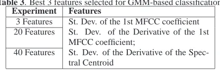
[image:4.595.316.538.612.684.2]The classification experiments were made using 7-fold cross validation, for the four NMF algorithms described in Section 3, for the GMM-based system described in Section 4 and for the continu-ous HMM-based system in Section 5. For the GMM system, three experiments were performed, using 3, 20 and 40 features. The mean classification rate for all eight experiments along with the standard deviation is presented in Figure 1. Using the automatic feature selection algorithm, the three best features selected for the three GMM classification experiments are presented in Table 3.
Table 3. Best 3 features selected for GMM-based classification. Experiment Features
3 Features St. Dev. of the 1st MFCC coefficient 20 Features St. Dev. of the Derivative of the 1st
MFCC coefficient;
40 Features St. Dev. of the Derivative of the Spec-tral Centroid
Classification algorithm
M
ea
n
cla
ss
ific
atio
n
ac
cu
ra
cy
%
NMF LNMF SNMF DNMF GMM3 GMM20 GMM40 HMM 0.9
0 10 20 30 40 50 60 70 80 90 100
Fig. 1. Classification accuracy for the tested algorithms.
[image:5.595.83.254.74.208.2]the systems with classification accuracy over 95% are the ones us-ing Standard NMF, GMMs (all 3 experiments) and the HMMs. It should be noted that the LNMF, SNMF and DNMF algorithms perform classification with rates well below 95%, which indicates that parts-based descriptors are not suitable for classifying holistic descriptors, whereas the more holistic NMF classifier displayed satisfactory results. More detailed information about the perfor-mance of the various algorithms is shown in Tables 4, 5 and 6 in the form of a confusion matrix, where the columns correspond to the predicted musical instrument and the rows to the actual one. For the Standard NMF algorithm, most misclassifications occur for the flute, while for the HMM-based system other instruments are misclassified as cello. It can be seen in table 5 that for the GMM classifier using 20 features, no misclassifications occur.
Table 4. Confusion matrix for one pass of the Standard NMF. Instr. Piano Bassoon Cello Flute Sax Violin
Piano 18 0 0 0 0 0
Bassoon 1 8 0 0 0 0
Cello 0 0 16 0 0 0
Flute 2 1 0 6 0 0
Sax 0 0 0 0 9 0
[image:5.595.308.549.86.170.2]Violin 0 0 0 0 0 29
Table 5. Confusion matrix for one pass of the GMM with 20
fea-tures.
Instr. Piano Bassoon Cello Flute Sax Violin
Piano 18 0 0 0 0 0
Bassoon 0 9 0 0 0 0
Cello 0 0 16 0 0 0
Flute 0 0 0 9 0 0
Sax 0 0 0 0 9 0
Violin 0 0 0 0 0 29
7. CONCLUSIONS
[image:5.595.48.290.553.665.2]In this paper, we have compared three systems for classifying mu-sical instrument recordings, the first using subspace analysis and the other two utilizing statistical model-based algorithms. A vari-ety of features used in audio classification experiments were used
Table 6. Confusion matrix for one pass of the HMM. Instr. Piano Bassoon Cello Flute Sax Violin
Piano 18 0 0 0 0 0
Bassoon 0 9 0 0 0 0
Cello 0 0 16 0 0 0
Flute 0 0 1 8 0 0
Sax 0 0 0 0 9 0
Violin 0 0 1 0 0 28
along with MPEG-7 descriptors. Results indicate that all three systems can perform classification with over 95% accuracy, out-performing state-of-the-art systems.
8. REFERENCES
[1] University of Iowa Musical Instrument Sample Database, http://theremin.music.uiowa.edu/index.html.
[2] MPEG-7 overview (version 9), ISO/IEC JTC1/SC29/WG11
N5525, March 2003.
[3] A. T. Lindsay, I. Burnett, S. Quackenbush, and M. Jack-son, “Fundamantals of Audio Descriptors”, in Introduction
to MPEG-7, (B.S.Manjuntath, P.Salembier and T.Sikora), pp.
285-298, Eds. New York: Wiley, 2000.
[4] H. G. Kim, N. Moreau, and T. Sikora, “Audio classifica-tion based on MPEG-7 spectral basis representaclassifica-tions,” IEEE
Trans. Circuits and Systems for Video Technology, vol. 14,
no. 5, pp. 716-725, May 2004.
[5] D. D. Lee and H. S. Seung, “Algoritnms for non-negative matrix factorization,” Advances in Neural Information
Pro-cessing Systems, vol. 13, pp. 556-562, 2001.
[6] S. Z. Li, X. Hou, H. Zhang, and Q. Cheng, “Learning spa-tially localized, parts-based representation,” in Proc. IEEE
Conf. Computer Vision and Pattern Recognition, pp. 1-6,
2001.
[7] C. Hu, B. Zhang, S. Yan, Q. Yang, J. Yan, Z. Chen, and W. Ma, “Mining ratio rules via principal sparse non-negative matrix factorization,” in Proc. IEEE Int. Conf. Data Mining, 2004.
[8] I. Buciu and I. Pitas, “A new sparse image representation al-gorithm applied to facial expression recognition,” in Proc.
17th Int. Conf. Pattern Recognition, August 2004.
[9] G. Tzanetakis and P. Cook, “Musical genre classification of audio signals,” IEEE Trans. Speech and Audio Processing, vol. 10, no. 5, pp. 293-302, July 2002.
[10] J. C. Brown, O. Houix, and S. McAdams, “Feature depen-dence in the automatic identification of musical woodwind instruments,” J. Acoustical Society of America, vol. 109, no. 3, pp. 1064-1072, March 2001.
[11] A. Wieczorkowska, J. Wroblewski, P. Synak, and D. Slezak, “Application of temporal descriptors to musical instrument sound recognition,” J. Intelligent Information Systems, vol. 21, no. 1, pp. 71-93, July 2003.
[12] J.J. Burred and A. Lerch, “Hierarchical automatic audio sig-nal classification,” J. Audio Engineering Society, vol. 52, no.7, 2004.
[13] S. B. Davis and P. Mermelstein, “Comparison of parametric representations for monosyllabic word recognition in contin-uously spoken sentences,” IEEE Trans. Acoust. Speech
Sig-nal Processing, vol. 28, no. 4, pp. 357-366, 1980.