City, University of London Institutional Repository
Citation:
Anderson, L. B., He, Y. and Lukas, A. (2007). Heterotic compactification, an algorithmic approach. Journal of High Energy Physics, 0707(049), doi: 10.1088/1126-6708/2007/07/049This is the unspecified version of the paper.
This version of the publication may differ from the final published
version.
Permanent repository link:
http://openaccess.city.ac.uk/870/Link to published version:
http://dx.doi.org/10.1088/1126-6708/2007/07/049Copyright and reuse: City Research Online aims to make research
outputs of City, University of London available to a wider audience.
Copyright and Moral Rights remain with the author(s) and/or copyright
holders. URLs from City Research Online may be freely distributed and
linked to.
City Research Online: http://openaccess.city.ac.uk/ [email protected]
arXiv:hep-th/0702210v2 23 May 2007
Heterotic Compactification, An Algorithmic Approach
Lara B. Anderson
1,3, Yang-Hui He
1,2, Andr´e Lukas
31 Mathematical Institute, Oxford University,
24-29 St. Giles’, Oxford OX1 3LB, U.K.
2Merton College, Oxford, OX1 4JD, U.K.
3Rudolf Peierls Centre for Theoretical Physics, Oxford University,
1 Keble Road, Oxford, OX1 3NP, U.K.
Abstract
We approach string phenomenology from the perspective of computational algebraic geometry, by providing new and efficient techniques for proving stability and calculating particle spectra in heterotic compactifications. This is done in the context of complete intersection Calabi-Yau manifolds in a single projective space where we classify positive monad bundles. Using a combination of analytic methods and computer algebra we prove stability for all such bundles and compute the complete particle spectrum, includ-ing gauge sinclud-inglets. In particular, we find that the number of anti-generations vanishes for all our bundles and that the spectrum is manifestly moduli-dependent.
Contents
1 Introduction 2
2 Heterotic Compactification and Physical Constraints 4
3 Monad Construction of Vector Bundles 7
3.1 The Calabi-Yau Spaces . . . 7
3.2 Constructing the Monad . . . 9
3.3 Stability of Monad Bundles . . . 12
4 Classification and Examples 14 4.1 Classification of Configurations . . . 15
4.2 E6-GUT Theories . . . 16
4.2.1 Particle Content . . . 16
4.3 SO(10)-GUT Theories . . . 20
4.3.1 Particle Content . . . 20
4.4 SU(5)-GUT Theories . . . 22
4.4.1 Stability for Rank 5 Bundles on the Quintic . . . 23
4.4.2 The Co-dimension 2 and 3 Manifolds . . . 24
4.4.3 Particle Content . . . 25
5 Conclusion 26 A Monads, Sheaf Cohomology and Computational Algebraic Geometry 27 A.1 The Sheaf-Module Correspondence . . . 28
A.2 Constructing Monads using Computer Algebra . . . 29
A.3 Algorithms for Sheaf Cohomology . . . 29
A.4 A Tutorial . . . 29
B Some useful technical results 31 B.1 Genericity of Maps . . . 31
B.2 Proof ofH0(X, V) = 0 . . . . 31
B.3 Proof that n1=h1(X,∧2V∗) = 0 for theSO(10) Models . . . 32
1
Introduction
Compactification of the E8 ×E8 heterotic string on Calabi-Yau three-folds [1, 2] is
building is still a long way away from one of its major goals: finding an example which does not merely have standard model spectrum but reproduces the standard model exactly, including detailed properties such as, for example, Yukawa couplings.
One of the main obstacles in achieving this goal is the inherent mathematical diffi-culty of heterotic models. In addition to a Calabi-Yau three-fold X, heterotic models require two holomorphic (semi)-stable vector bundles V and ˜V on X. Except for the simple case of standard embedding, where V is taken to be the tangent bundle T X
of the Calabi-Yau space and ˜V is trivial, construction of these vector bundles is often not straightforward and the computation of their properties is usually involved. For example, stability of these bundles, an essential property if the model is to preserve supersymmetry, is notoriously difficult to prove. In addition, when searching for realis-tic parrealis-ticle physics from heterorealis-tic string theory, these mathemarealis-tical obstacles have to be resolved for a large number of Calabi-Yau spaces and associated bundles, as every single model (or even a small number of models) is highly likely to fail when confronted with the detailed structure of the standard model. The main purpose of this paper is to present an algorithmic approach to this problem by combining analytic methods and computer algebra. By an algorithmic approach we mean a set of techniques which allow us to construct classes of vector bundles on (certain) Calabi-Yau spaces systematically, prove their stability and compute the resulting low-energy particle spectra completely. In this paper we will focus on developing the necessary computational methods by con-centrating on the five Calabi-Yau manifolds which can be obtained by intersections in an ordinary projective space. A generalization of these methods to more general com-plete intersection Calabi-Yau manifolds and a detailed analysis of the particle physics properties of these models will be the subject of forthcoming publications [9].
Starting with the pioneering work in [10, 11], there has been continuing activity on Calabi-Yau based non-standard embedding models over the years. Recently, there has been significant progress both from the mathematical and the model-building viewpoint, leading to models edging closer and closer towards the standard model [4, 5]. Two types of constructions, one based on elliptically fibered Calabi-Yau spaces with bundles of the Friedman-Morgan-Witten type [12] and generalizations [3]–[8], [13]–[15], the other based on complete intersection Calabi-Yau spaces with monad bundles [11], [16]–[19], have been pursued in the literature. In this paper, we will work within the context of the second approach using complete intersection Calabi-Yau manifolds and monad bundles. To explain our motivation for this choice we remind the reader of the usual “two-step” symmetry breaking in heterotic models. In the first step, the E8 gauge
group is broken to one of the standard grand unified groups E6, SO(10) or SU(5) by
discrete symmetry group is greatly facilitated by the presence of an ambient projective space. This is one of our main motivations for working with this class of manifolds, although analyzing discrete symmetries and Wilson line breaking explicitly will be the subject of a future publication [9]. Another major reason for our choice of models is that all relevant objects can be readily described in the language of commutative algebra and, therefore, lent themselves to an analysis based on computer algebra.
In this paper, we will construct all positive monad bundles of rank 3, 4 and 5 on the five complete intersection Calabi-Yau spaces in a single projective space subject to two additional constraints. First, the bundles should be such that heterotic anomaly cancellation can be accomplished and second, their chiral asymmetry should be a (non-zero) multiple of three. We find 37 examples in total. We then prove stability for all these bundles using a variant of a simple criterion due to Hoppe [21]. Recently, this criterion has been used [22], although in a slightly different way from the present paper, to prove stability for a class of positive bundles on the quintic [19]. Further, we compute the complete spectrum for all bundles, including gauge singlet fields. It turns out that a common feature of our models is that they only lead to generations but no anti-generations. While the present paper deals with a relatively small number of examples, we have shown that the relevant methods can be applied in a systematic and algorithmic way. We expect that a significantly larger class of complete intersection Calabi-Yau spaces and bundles on them can be treated in a similar way (see [20] for a recent constraint on classifying bundles in general). This generalization and the analysis of the particle physics of the resulting models will be the subject of future work [9].
The plan of the paper is as follows. In the next section, we will briefly review the main general features ofE8×E8heterotic compactifications. In Section 3, we discuss the
monad construction, its main properties and prove a number of general results for such bundles. In Section 4, we classify the positive monad bundles on our five Calabi-Yau spaces, prove their stability and compute the spectra. After our conclusions in Section 5, Appendix A follows with a short summary of the relevant tools in commutative algebra and how they are applied in the context of the Macaulay computer algebra package [23]. The final Appendices contain several useful technical results.
2
Heterotic Compactification and Physical
Con-straints
To set the scene, we would now like to briefly review the basic structure of E8 ×E8
heterotic vacua on Calabi-Yau three-folds (see Ref. [28, 6, 8]).
In addition to a Calabi-Yau three-fold X with tangent bundle, T X, we need two holomorphic vector bundles V and ˜V with associated structure groups which are sub-groups ofE8. In the present context, we will be interested in bundles with rankn= 3,4,5
contain five-branes which appear as M five-branes in the 11-dimensional strong-coupling limit and as NS 5-branes in the 10-dimensional weakly coupled theory. In either case, for a supersymmetric compactification, the five-branes have to wrap a holomorphic curve in the Calabi-Yau space X, whose second homology class we denote byW ∈H2(X,Z).
Two additional conditions need to be imposed on this data if the associated com-pactification is to preserve N = 1 supersymmetry in four dimensions. First, the two bundles V and ˜V need to be (semi-) stable bundles [29]. To introduce the notion of stability, we define the slope
µ(F) = 1 rk(F)
Z
X
c1(F)∧J∧J (1)
of a (coherent) sheaf F on X, where J is the K¨ahler form on X and rk(F) and c1(F)
are the rank and the first Chern class of the sheaf, respectively. A bundle V is now called stable (resp. semi-stable) if for all sub-sheafs F ⊂ V with 0 < rk(F) < rk(V) the slope satisfies µ(F) < µ(V) (resp. µ(F) ≤ µ(V)). It is worth mentioning that a bundleV is semi-stable exactly if its dualV∗
is and thath0(X, V) =h3(X, V) = 0 for a
stable bundle V. To preserve supersymmetry, semi-stability of the bundle is sufficient, although in practice one often requires stability. For specific examples, either condition is typically very hard to check and the stability proof for the bundles considered in this paper, is one of our main results. In addition, for supersymmetry to be preserved, the five-brane class W needs to be an effective class. This means that there indeed exists a holomorphic curve with class W inX.
Finally, heterotic models need to satisfy a well-known anomaly condition. For the case of bundles V and ˜V with vanishing first Chern classes, c1(V) = c1( ˜V) = 0, which
we consider in this paper this condition reads
c2(T X)−c2(V)−c2( ˜V) =W . (2)
Next, we turn to the general structure of the low-energy particle spectrum. In addition to the dilaton, h1,1(X) K¨ahler moduli and h2,1(X) complex structure moduli
of the Calabi-Yau space, each of theE8 gauge theories as well as the five-branes give rise
to a sector of particles in the low-energy theory. Here, we will focus on the “observable” sector, associated to the firstE8gauge theory with vector bundleV and structure group G. We will not explicitly consider the particle content in the other “hidden” sectors.
The low-energy gauge groupH in the observable sector is given by the commutant of the structure group G within E8. For G = SU(3), SU(4), SU(5) this implies the
standard grand unified groups H = E6, SO(10), SU(5), respectively. In order to find
the matter field representations, we have to decompose the adjoint 248 of E8 under G×H. In general, this decomposition can be written as
248→(1,Ad(H))⊕M
i
E8 →G×H Residual Group Structure
SU(3)×E6 248 →(1,78)⊕(3,27)⊕(3,27)⊕(8,1)
SU(4)×SO(10) 248 →(1,45)⊕(4,16)⊕(4,16)⊕(6,10)⊕(15,1)
SU(5)×SU(5) 248 →(1,24)⊕(5,10)⊕(5,10)⊕(10,5)⊕(10,5)⊕(24,1)
Table 1: Breaking patterns of E8 and decompositions of the 248 adjoint representation.
Decomposition Cohomologies
SU(3)×E6 n27 =h1(V), n27=h1(V∗) =h2(V), n1 =h1(V ⊗V∗) SU(4)×SO(10) n16 =h1
(V), n16=h2
(V), n10 =h1 (∧2
V), n1 =h1
(V ⊗V∗ ) SU(5)×SU(5) n10 =h1(V∗
), n10=h1(V), n5 =h1(∧2V), n5 =h1(∧2V∗ ) n1 =h1(V ⊗V∗
)
Table 2: Computation of low-energy particle spectra.
where Ad(H) denotes the adjoint representation ofH and{(Ri, ri)}is a set of
represen-tations of G×H. The adjoint representation ofH corresponds to the low-energy gauge fields while the low-energy matter fields transform in the representationsriofH. For the
three relevant structure groups these matter field representations are explicitly listed in Table 1. We may ask how many supermultiplets will occur in the low energy theory for each representation ri? It turns out that this number is given by nri =h
1(X, V
Ri), the
dimension of the cohomology group H1(X, V
Ri) of the vector bundle V in the specific
G representation Ri which is paired up with theH representation ri in the
decomposi-tion (3). ForG= SU(n), the relevant representationsRi can be obtained by appropriate
tensor products of the fundamental representation and one ends up having to compute
h1(X, V ⊗V∗
), h1(X, V), h1(X, V∗
), h1(X,∧2V), and h1(X,∧2V∗
). Using Serre du-ality, h1(X, V∗
) = h2(X, V), the number the low-energy representations can then be
computed as summarized in Table 2. Further, the Atiyah-Singer index theorem [40], applied to the case c1(T X) =c1(V) = 0, tells us that the index ofV can be expressed
as
ind(V) =
3
X
p=0
(−1)php(X, V) = 1 2
Z
X
c3(V), (4)
where c3(V) is the third Chern class of V. For a stable bundle, we have h0(X, V) = h3(X, V) = 0 and comparison with Table 2 shows that, in this case, the index counts
the chiral asymmetry, that is, the difference of the number of generations and anti-generations. The index is usually easier to compute than individual cohomologies and is useful to impose a physical constraint on the chiral asymmetry.
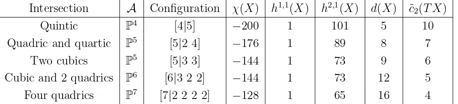
Intersection A Configuration χ(X) h1,1(X) h2,1(X) d(X) ˜c2(T X)
Quintic P4 [4|5] −200 1 101 5 10
Quadric and quartic P5
[5|2 4] −176 1 89 8 7
Two cubics P5
[5|3 3] −144 1 73 9 6
Cubic and 2 quadrics P6 [6|3 2 2] −144 1 73 12 5 Four quadrics P7
[image:8.612.72.529.37.141.2][7|2 2 2 2] −128 1 65 16 4
Table 3: The five complete intersection Calabi-Yau manifolds in a single projective space. Here, χ(X) is the Euler number, h1,1(X) and h2,1(X) are the Hodge numbers, d(X) is the intersection number and c2(T X) = ˜c2(T X)J2
is the second Chern class. The normalization of the K¨ahler form J is defined in the main text.
spaces realized as intersections in a single ordinary projective space), we will scan over a certain, well-defined class of (monad) bundles, V, on X. We will think of these bundles as bundles in the observable sector and take the hidden bundle ˜V to be trivial. The anomaly condition (2) can then be satisfied by including five-branes as long as
c2(T X)−c2(V) is an effective class on X. This is precisely what we will require. In
addition, we will only consider bundlesV whose index is a (non-zero) multiple of three. Only such bundles have a chance, after dividing out by a discrete symmetry, of producing a model with chiral asymmetry three. We will then prove stability for all such bundles and compute their complete low-energy spectrum.
3
Monad Construction of Vector Bundles
To begin our systematic construction of vector bundles for heterotic compactifications, we will make use of a standard and powerful technique for defining bundles, known as the monad construction. On complex projective varieties, this method of constructing vector bundles dates back to the early works on P4 by [33] and systematic approaches
by [34] and [35]. This construction defines a vast class of vector bundles; in fact, every bundle on Pn can be expressed as a monad [30, 33]. Bundles defined as monads have
been widely used in the mathematics and physics literature. The reader is referred to [36] for the most general construction of monads and their properties. In this work we will use a restricted form prevalent in the physics literature.
3.1
The Calabi-Yau Spaces
Our monad bundles will be constructed on complete intersection Calabi-Yau manifolds,
X, which are defined in a single projective ambient space A = Pm. There are five
wheremrefers to the dimension of the ambient spacePmand the numbersq
aindicate the
degree of the defining polynomials. In this notation the Calabi-Yau conditionc1(T X) =
0 translates to PKa=1qa=m+ 1. Furthermore, note that h1,1(X) = 1 for all five cases.
Hence, these manifolds have their Picard group, Pic(X), being isomorphic to Z. Such
manifolds are calledcyclic[32]. The K¨ahler formJ descends from the the ambient space
Pnand is normalized as
Z
Pn
Jm= 1. (5)
Integrals over X of any three-form w, defined on A=Pm, can be reduced to integrals
over the ambient space using the formula
Z
X
w=d(X)
Z
Pm
w∧Jm−3, (6)
where d(X) are the intersection numbers listed in Table 3. The second homology
H2(X,Z) is dual to the integer multiples of J∧J and the Mori cone of X corresponds
to all positive multiples of J∧J [25].
For our subsequent analysis it is useful to discuss some properties of line bundles on the above Calabi-Yau manifolds. We denote by O(k) the kth power of the hyperplane
bundle, O(1), on the ambient space Pm and by O
X(k) its restriction to the Calabi-Yau
space X. The normal bundleN of X in the ambient space is then given by
N =
K
M
a=1
O(qa). (7)
In general, one finds, for the Chern characters of line bundles on X,
ch1(OX(k)) = c1(OX(k)) =kJ , (8)
ch2(OX(k)) =
1 2k
2
J2 , (9)
ch3(OX(k)) =
1 6k
3
J3. (10)
From the Atiyah-Singer index theorem the index of OX(k) is given by
ind(OX(k)) ≡ 3
X
q=0
(−1)qhq(X,O X(k))
=
Z
X
ch3(OX(k)) +
1
12c2(T X)∧c1(OX(k))
= d(X)k 6
k2+ 1
2c˜2(T X)
, (11)
where the numbers ˜c2(T X) characterize the second Chern class of X and d(X) are the
intersection numbers. The values for these quantities can be read off from Table 3. We recall that the Kodaira vanishing theorem [40] states that on a K¨ahler manifold
X, Hq(X, L⊗K
X) vanishes for q > 0 and L a positive line bundle. Here, KX is the
the only non-vanishing cohomology for positive line bundles on Calabi-Yau manifolds is H0. The dimension of this cohomology group can then be computed from the index
theorem. In fact, inserting the values for the intersection numbers and the second Chern class from Table 3 into Eq. (11) we explicitly find, for the five Calabi-Yau spaces and for line bundles OX(k) withk >0, that
h0([4|5],OX(k)) =
5 6(k
3
+ 5k) , (12)
h0([5|2 4],O
X(k)) =
2 3(2k
3+ 7k) , (13)
h0([5|3 3],OX(k)) =
3 2(k
3
+ 3k) , (14)
h0([6|3 2 2],OX(k)) = 2k3+ 5k , (15) h0([7|2 2 2 2],OX(k)) =
8 3(k
3
+ 2k). (16)
For negative line bundlesL=OX(−k), wherek >0, it follows from Serre duality on the
Calabi-Yau three-fold X,hq(X, L) =h3−q(X, L∗
), that onlyH3(L, X) can be non-zero
and that its dimension h3(X,O
X(−k)) = h0(X,OX(k)) is given by one of the explicit
expressions (12)–(16). Finally, we have
h0(X,OX) =h3(X,OX) = 1 , h1(X,OX) =h2(X,OX) = 0. (17)
Now we explicitly know the cohomology for all line bundles on the five Calabi-Yau man-ifolds under consideration. In particular, we conclude that h0(X,O
X(k))>0 precisely
for k ≥ 0 and, hence, that only the line bundlesOX(k) with k ≥ 0 have a non-trivial
section. This is one of the underlying conditions for the validity of Hoppe’s criterion which will play a central role in the stability proof for our bundles.
3.2
Constructing the Monad
Having discussed the manifoldX and line bundles thereon, we now construct the requi-site vector bundlesV. Our construction proceeds as follows. On a Calabi-Yau manifold
X, a monad bundleV is defined by the short exact sequence
0→V −→f B −→g C →0, (18)
where B andC are bundles onX. It is standard to take B and C to be direct sums of line bundles over X, that is
B=
rB
M
i=1
OX(bi), C= rC
M
i=1
OX(ci). (19)
Here, rB and rC are the ranks of the bundles B and C, respectively. The exactness of
(18) implies that ker(g) = im(f) and ker(f) = 0, so that the bundleV can be expressed as
The mapgis a morphism between bundles and can be defined as arC×rBmatrix whose
entries, (i, j), are sections ofOX(ci−bj). As we have seen in the previous subsection,
such sections exist iff ci ≥bj and so this is what we should require. In fact, ifci =bj
for an index pair (i, j) the two corresponding line bundles can simply be dropped from
B and C without changing the resulting bundleV. In the following, we will, therefore, assume the stronger condition ci > bj for all iand j.
The Calabi-Yau manifolds discussed in this paper are complete intersections in a single projective space Pm. We can, therefore, write down an analogous short exact
sequence
0→ V −→ Bf˜ −→ C →g˜ 0, (20) on the ambient space where
B=
rB
M
i=1
O(bi), C= rC
M
i=1
O(ci). (21)
The map ˜g can be viewed as a rC ×rB matrix whose entries, (i, j), are homogeneous
polynomials of degree ci−bj. This sequence defines a vector bundleV on the ambient
space whose restriction to X is V. Further, the mapg can be seen as the restriction of its ambient space counterpart ˜gtoX. Unless explicitly stated otherwise, we will assume throughout that this map is generic.
It is natural to enquire whether V thus defined is always a bona fide bundle rather than a sheaf. We are assured on this point by the following theorem [42].
THEOREM 3.1 Over any smooth varietyX, ifg:B →C is a morphism between locally free sheaves B and C, then ker(g) is locally free.
Now, by definition, a locally free sheaf of constant rank is a vector bundle. Therefore, by the above theorem, it only remains to check whether ker(g) has constant rank on X. Indeed,gcould be less than maximal rank on a singular (sometimes called ‘degeneracy’) locus. We note that exactness of the sequence, that is coker(g) = 0, is equivalent to this degeneracy locus being empty.
To show that the degeneracy locus is empty for our bundles, it turns out to be convenient to consider the dual bundleV∗
defined by the dual sequence
0→C∗ gT
−→B∗
−→V∗
→0, (22)
where
V∗
= coker(gT). (23) We can now apply the following theorem [22, 45].
THEOREM 3.2 Let φ:E →F be a morphism of vector bundles on a variety of dimen-sion N and let e= rk(E), f = rk(F) and e ≤f. If E∗
⊗F is globally generated and
Therefore, take φ =gT, E =C∗
and F =B∗
. For all our bundles of interest, N = 3 and e < f. In fact, f−eis the rank of V, which is 3, 4, or 5 for the bundles of interest in heterotic compactifications. Finally, E∗
⊗F is globally generated because B and C
are direct sums of line bundles with ci > bj for all i, j. Hence, all the conditions in the
theorem are obeyed and we see that the degeneracy locus of gT, and hence the one for g, is vanishing for the bundles of interest on the Calabi-Yau. However, one should note that this criterion will not always be satisfied when writing monad sequences on the higher dimensional ambient spaces, as in Eq. (20). (Such issues will be discussed further in section 4.4). For more on the degeneracy locus of bundle maps, and why Theorem 3.2 guarantees its vanishing in the dual monad, see e.g. [43, 44].)
For later reference we present the formulae for the Chern classes ofV (see Ref. [31]). Simplifying the expressions for c2(V) and c3(V) by imposing the vanishing of the first
Chern class, we have
rk(V) = rB−rC , (24) c1(V) =
rB
X
i=1 bi−
rC
X
i=1 ci
!
J ≡0 , (25)
c2(V) = −
1 2 rB X i=1 b2 i − rC X i=1 c2 i !
J2 , (26)
c3(V) =
1 3 rB X i=1 b3 i − rC X i=1 c3 i !
J3 . (27)
Hence, from Eq. (4) and the above expression for the third Chern class, the index of V
is explicitly given by
ind(V) =
3
X
p=0
(−1)php(X, V) = d(X) 6 rB X i=1 b3 i − rC X i=1 c3 i ! . (28)
Within this paper, we will make extensive use of the computer algebra system [23] in analyzing the monads in (18). Utilizing this powerful tool we are able to catalog efficiently bundle cohomologies previously too difficult to be calculated. Indeed, com-puting particle spectra, that is, sheaf cohomology, is ordinarily a tremendous task even for a single bundle, and it would be unthinkable to attempt to calculate by hand the hundreds of such cohomologies necessary in a systematic study of monad bundles. How-ever, the recent advances in algorithmic algebraic geometry allow us to explicitly and efficiently compute the requisite cohomology groups for a certain class of bundles. For the first time, we describe in detail how to use this technology in the context of string compactification.
With this approach in mind, we recall that in computational algebraic geometry [38], sheafs are expressed in the language of graded modules over polynomial rings. If
X is embedded in Pm with homogeneous coordinates [x
0 : x1 : . . . : xm], we can let R be the coordinate ring C[x0, x1, . . . , xm]/(X) where (X) is the ideal associated with
degrees (grading). We leave to the Appendix a detailed tutorial of the sheaf-module correspondence and the construction and relevant computation of monad bundles using computer algebra.
3.3
Stability of Monad Bundles
As mentioned in the previous section, (semi-)stability of the vector bundle is of central importance to heterotic compactifications. In general, proving stability is an overwhelm-ing technical obstacle and a systematic analysis has so far been elusive. However, for a class of manifolds, a sufficient but by no means necessary condition is of great utility; this is the so-called Hoppe’s criterion [21, 37]:
THEOREM 3.3 [Hoppe’s Criterion] Over a projective manifold X with Picard group
P ic(X)≃Z(i.e.,Xis cyclic), letV be a vector bundle withc1(V) = 0. IfH0(X,Vp V) = 0 for all p= 1,2, . . . ,rk(V)−1, then V is stable.
We also recall that for the Calabi-Yau manifolds used in this paper all positive line bundles have a section, an underlying assumption for the validity of Hoppe’s theorem which is, hence, satisfied.
The strategy is therefore clear. To prove stability for the monad bundles (18) over cyclic manifoldsXusing Hoppe’s criterion, we need to show the vanishing ofH0(X,∧pV)
for p= 1, . . . ,rk(V)−1. In the following paragraphs, we will outline the basis for this stability proof and make note of certain results and properties that are of particular use. One additional assumption which we will make is that all line bundles involved in the definition of the bundlesV are positive, that is, for alli,
bi >0 andci >0. (29)
We will refer to this property as “positivity” of the bundleV. While this is not required for a consistent definition of the bundle or the associated heterotic model, it turns out to be a crucial technical assumption which facilitates the stability proof. The essential point is that positivity ofV allows one to use Kodaira vanishing when applying Hoppe’s criterion to the dual bundle V∗
. To see how this works, recall that the dual bundle is defined by the sequence 0→C∗ −→B∗ −→V∗ →0 and that its stability is equivalent
to that of V. The associated long exact sequence in cohomology is 0 → H0(X, C∗
)→H0(X, B∗
)→ H0(X, V∗)
→ H1(X, C∗
)→H1(X, B∗
)→H1(X, V∗
)
→ H2(X, C∗
)→H2(X, B∗
)→H2(X, V∗
)
→ H3(X, C∗
)→H3(X, B∗
)→H3(X, V∗
)→0 . (30)
Given that we are dealing with positive bundles V, it follows thatB∗
and C∗
are sums of negative line bundles and, hence, H0(X, B∗
) and H1(X, C∗
also vanishes. (For later considerations we note that Kodaira vanishing also implies
H1(X, B∗
) =H2(X, C∗
) = 0 and, hence,H1(X, V∗
)≃H2(X, V) = 0.) In order to prove
stability of V∗
by applying Hoppe’s criterion we have to show that H0(X,∧pV∗
) = 0 forp= 1, . . . ,rk(V)−1 and we have just completed the first step forp= 1.
Next, we need to compute the cohomologies H0X,∧pV∗
) for p > 1. However, a further simplification occurs because we are dealing with unitary bundles. In fact, for an SU(n) bundle V, we have
∧n−1V∗
≃V (31)
(see, for example Ref. [41]) . Therefore, to cover the case p=n−1, the highest exterior power relevant to Hoppe’s criterion, we only need to show that H0(X, V) = 0. This is
indeed the case for all bundles considered in this paper and the explicit proof, which is somewhat lengthy, is presented in Appendix B.2. This completes the stability proof for the rank 3 bundles.
For rank 4 and 5 bundles we have to look at further exterior powers of V∗
, namely ΛpV∗
forp= 2, . . . ,rk(V)−2. To deal with those we consider the standard long exact (“exterior power”) sequence [22, 40] for ΛpV∗
0 → SpC∗
→Sp−1C∗
⊗B∗
→Sp−2C∗
⊗ ∧2 B∗
→. . .
→ A⊗ ∧p−1B∗
→ ∧pB∗
→ ∧pV∗
→0 , (32)
which is induced by the short exact sequence (22). Here Si is the i-th symmetrised
tensor power of a bundle. Such a sequence does not itself induce a long exact sequence in cohomology; we need to slice it up into groups of three. In other words, we introduce co-kernels Ki such that (32) becomes the following set of short exact sequences
0 → SpC∗
→Sp−1C∗
⊗B∗
→K1→0 ,
0 → K1 →Sp−2C ∗
⊗ ∧2B∗
→K2 →0 ,
.. .
0 → Kp−1 → ∧pB∗ → ∧pV∗→0 . (33)
Each of the above now induces a long exact sequence in cohomology in analogy to (30): 0→H0(X, SpC∗)→H0(X, Sp−1C∗⊗B∗)→H0(X, K
1)→H1(X, SpC∗)→. . .→0 ,
0→H0(X, K
1)→H0(X, Sp−2C∗⊗ ∧2B∗)→H0(X, K2)→H1(X, K1)→. . .→0 ,
.. . 0→H0(X, K
p−1)→H0(X,∧pB∗)→ H0(X,∧pV∗) →H1(X, Kp−1)→. . .→0.
(34) The term we need is boxed and we need to trace through the various sequences, using the readily computed cohomologies of the symmetric and antisymmetric powers of B∗
and C∗
, to arrive at the answer. Let us now do this explicitly for the case p= 2, that is, H0(X,Λ2V∗
). The long exact sequence (32) then specializes to 0→S2C∗
→C∗
⊗B∗
→Λ2B∗
→Λ2V∗
which needs to be broken up into the two short exact sequences
0 →S2C∗
→C∗
⊗B∗
→K →0 (36)
0 →K →Λ2B∗
→Λ2V∗
→0. (37)
From the first of these we have the long exact sequence
0 → H0(X, S2C∗
)→H0(X, C∗
⊗B∗
)→H0(X, K)
→ H1(X, S2C∗
)→H1(X, C∗
⊗B∗
)→H1(X, K)
→ H1(X, S2C∗
)→. . . . (38)
Since B∗
and C∗
are sums negative line bundles, so are their various tensor products which appear in the above sequences. From Kodaira vanishing all cohomologies of such bundles vanish except for the third. Applying this to (38) we immediately deduce that
H0(X, K) =H1(X, K) = 0. Using this information in the long exact sequence
0→H0(X, K)→H0(X,Λ2B∗
)→H0(X,Λ2V∗
)→H1(X, K)→. . . (39)
which follows from (37) we find H0(X,Λ2V∗
) = 0, as desired. This completes the stability proof for rank 4 bundles1.
Finally, for rank 5 bundles, we still need to compute H0(X,Λ3V∗
). Repeating the above steps for this case one finds that Kodaira vanishing on X alone does not quite provide sufficient information to conclude that H0(X,Λ3V∗) = 0. In this case, we
need to employ the additional technique of Koszul sequences [31, 40] which rely on the embedding of the Calabi-Yau manifold in an ambient spaceA. Specifically, for a vector bundleW on Athe Koszul sequence reads
0→ ∧KN∗
⊗ W →...→ ∧2N∗
⊗ W → N∗
⊗ W → W → W|ρ X →0, (40)
where W|X denotes the restriction of W to X and ρ is the associated restriction map.
Here N∗
is the dual of the Calabi-Yau normal bundle, defined in Eq. (7). As will be shown in the next section, the Koszul sequence can be used to compute the relevant co-homologies directly from the ambient space. This will allow us to complete the stability proof for rank 5 bundles.
4
Classification and Examples
Armed with the general information about the five Calabi-Yau manifolds and monad bundles we can now proceed to classify such bundles, prove their stability and compute their spectrum.
1
Together with H0
4.1
Classification of Configurations
For the monad bundles defined by the short exact sequence (18), we can immediately formulate a classification scheme. Recall that, taking the bundlesB andC to be direct sums of line-bundles over the manifold X, we have
0→V →
rB
M
i=1
OX(bi) g
−→
rC
M
i=1
OX(ci)→0 , V ≃ker(g) . (41)
From our discussion so far these bundles are subject to a number of physical and math-ematical constraints which can be summarised as follows:
1. As discussed earlier we require all bi and ci to be positive; this is a technical
assumption which will significantly simplify our computations.
2. We furthermore require thatbi < cj for all iand j; this is to ensure that the map g, which consists of sections ofOX(cj−bi), has no zero entries. Further, we require
the map g to be generic. Then, all conditions of Theorem (3.2) are met and we are guaranteed that V, as defined by the sequence (41), is indeed a bundle. 3. Since we are dealing with special unitary bundles we imposec1(V) = 0.
4. For a given Calabi-Yau spaceXand a bundleV we need to ensure that the anomaly condition (2) can be satisfied. To do this we impose the condition that c2(T X)− c2(V) must be effective. Then, we can choose a trivial hidden bundle ˜V and a
five-brane wrapping a holomorphic curve with homology classc2(T X)−c2(V). In
practice, this condition simply means that the coefficient ofJ2 inc
2(T X)−c2(V)
must be non-negative 2 .
5. We require that the index ofV is a non-zero multiple of three. Only such models may lead to three generations after dividing by a discrete symmetry.
6. Since we are interested in low-energy grand unified groups we consider bundlesV
with structure group SU(n), wheren= rk(V) = 3,4,5.
Therefore, an integer partitioning problem immediately presents itself to us: find parti-tions{bi}i=1,...,rC+nand {cj}i=1,...,rC of positive integersbi >0,ci>0 satisfyingbi < cj
for all i,j and subject to the condition
rB
P
i=1 bi−
rC
P
i=1
ci = 0 for vanishing first Chern class
of V (see Eq. (25)). Further, we demand that the index ofV, Eq. (28), is non-zero and divisible by three and that the coefficient of J2 in c
2(T X)−c2(V) be non-negative, in
order to ensure the existence of a holomorphic five-brane curve. From Eq. (26) the last constraint can be explicitly written as
0≤ −1
2(
rXC+n
i=1 bi−
rC
X
i=1
ci)≤c˜2(T X), (42)
2
where the numbers ˜c2(T X) for the second Chern class ofX are given in Table 3. Since bi < cj for all i, j it is clear that this constraint implies an upper bound on bi and cj
and, hence, that the number of vector bundles in our class is finite 3. To derive this
bound explicitly we slightly modify an argument from Appendix B of Ref. [19]. Define the quantity
S =
rXC+n
i=1 bi=
rC
X
i=1
ci , (43)
and consider the following chain of inequalities
2 ˜c2(T X)≥ rC
X
i=1 c2i −
rXC+n
i=1
b2i ≥ (bmax+ 1) rC
X
i=1 ci−
rXC+n
i=1 b2i
= S+
rXC+n
i=1
bmaxbi− rXC+n
i=1
b2i ≥S .
From Table 3, ˜c2(T X) is at most 10 and, hence, the sum S cannot exceed 20, thereby
placing an upper bound on our partitioning problem.
Given the finiteness of the problem, the classification of all positive monad bundles subject to the above constraints is now easily computerisable. Given these conditions, we found 37 bundles on the five Calabi-Yau manifolds in question, 20 for rank 3, 10 for rank 4 and 7 for rank 5. Had we relaxed the condition that c3 should be divisible by 3,
we would have found 43, 15, 10, 6, and 3 bundles, respectively on the 5 cyclic manifolds, for a total of 77. A complete list of all such bundles for the five Calabi-Yau manifolds of concern is given in the Tables 4–8.
4.2
E
6-GUT Theories
The first case we shall analyse isE6-GUT theories which arise fromSU(3) bundles. We
have already seen in Section 3.3 that all such bundles are indeed stable. This result has been explicitly confirmed by a computer algebra computation of H0(X, V∗) and H0(X,Λ2V∗
) along the lines described in Appendix A. We can, therefore, directly turn to a computation of their particle spectrum.
4.2.1 Particle Content
The number of 27 and 27 representation of E6 is easy to obtain. Since V is stable
we already know that H0(X, V) = H3(X, V) = 0. From the long exact sequence (30)
we have deduced earlier that H2(X, V)≃H1(X, V∗
) = 0 so that H1(X, V) is the only
non-vanishing cohomology. Its dimension can be directly computed from the index (28), so that
n27=h1(X, V) =−ind(V), n27=h 2
(X, V) = 0. (44)
3
Rank {bi} {ci} c2(V)/J2 ind(V)
3 (2, 2, 1, 1, 1) (4, 3) 7 -60
3 (2, 2, 2, 1, 1) (5, 3) 10 -105
3 (3, 2, 1, 1, 1) (4, 4) 8 -75
3 (1, 1, 1, 1, 1, 1) (2, 2, 2) 3 -15
3 (2, 2, 2, 1, 1, 1) (3, 3, 3) 6 -45
3 (3, 3, 3, 1, 1, 1) (4, 4, 4) 9 -90
3 (2, 2, 2, 2, 2, 2, 2, 2) (4, 3, 3, 3, 3) 10 -90 3 (2, 2, 2, 2, 2, 2, 2, 2, 2) (3, 3, 3, 3, 3, 3) 9 -75
4 (2, 2, 1, 1, 1, 1) (4, 4) 10 -90
[image:18.612.106.489.87.368.2]4 (1, 1, 1, 1, 1, 1, 1) (3, 2, 2) 5 -30 4 (2, 2, 2, 1, 1, 1, 1) (4, 3, 3) 9 -75 4 (2, 2, 2, 2, 1, 1, 1, 1) (3, 3, 3, 3) 8 -60 5 (1, 1, 1, 1, 1, 1, 1, 1) (3, 3, 2) 7 -45 5 (1, 1, 1, 1, 1, 1, 1, 1) (4, 2, 2) 8 -60 5 (2, 2, 2, 2, 2, 1, 1, 1, 1, 1) (3, 3, 3, 3, 3) 10 -75
Table 4: Positive monad bundles on the quintic, [4|5].
Rank {bi} {ci} c2(V)/J2
ind(V) 3 (2, 2, 1, 1, 1) (4, 3) 7 -96 3 (1, 1, 1, 1, 1, 1) (2, 2, 2) 3 -24 3 (2, 2, 2, 1, 1, 1) (3, 3, 3) 6 -72 4 (1, 1, 1, 1, 1, 1, 1) (3, 2, 2) 5 -48 5 (1, 1, 1, 1, 1, 1, 1, 1) (3, 3, 2) 7 -72
[image:18.612.140.459.517.626.2]Rank {bi} {ci} c2(V)/J2 ind(V)
3 (1, 1, 1, 1) (4) 6 -90
3 (1, 1, 1, 1, 1) (3, 2) 4 -45
3 (2, 1, 1, 1, 1) (3, 3) 5 -63
3 (1, 1, 1, 1, 1, 1) (2, 2, 2) 3 -27 3 (2, 2, 2, 1, 1, 1) (3, 3, 3) 6 -81
4 (1, 1, 1, 1, 1, 1) (3, 3) 6 -72
[image:19.612.113.484.68.262.2]4 (1, 1, 1, 1, 1, 1, 1) (3, 2, 2) 5 -54 4 (1, 1, 1, 1, 1, 1, 1, 1) (2, 2, 2, 2) 4 -36 5 (1, 1, 1, 1, 1, 1, 1, 1, 1) (3, 2, 2, 2) 6 -63 5 (1, 1, 1, 1, 1, 1, 1, 1, 1, 1) (2, 2, 2, 2, 2) 5 -45
Table 6: Positive monad bundles on [5|3 3].
Rank {bi} {ci} c2(V)/J2 ind(V)
3 (1, 1, 1, 1, 1) (3, 2) 4 -60
3 (2, 1, 1, 1, 1) (3, 3) 5 -84
[image:19.612.113.486.373.496.2]3 (1, 1, 1, 1, 1, 1) (2, 2, 2) 3 -36 4 (1, 1, 1, 1, 1, 1, 1) (3, 2, 2) 5 -72 4 (1, 1, 1, 1, 1, 1, 1, 1) (2, 2, 2, 2) 4 -48 5 (1, 1, 1, 1, 1, 1, 1, 1, 1, 1) (2, 2, 2, 2, 2) 5 -60
Table 7: Positive monad bundles on [6|2 2 3].
Rank {bi} {ci} c2(V)/J2 ind(V) 3 (1, 1, 1, 1, 1, 1) (2, 2, 2) 3 -48
[image:19.612.155.444.608.645.2]Therefore, for the rank 3 bundles in Tables 4–8, the (negative of the) right-most column gives the number of 27 representations. This result also provides the first example of what is a general feature of positive monad bundles, namely the absence of anti-generations. The numbers n27 have been independently verified by computer algebra.
What about the E6 singlets? These correspond to the cohomology H1(X,ad(V)) = H1(X, V ⊗V∗
). We begin by tensoring the defining sequence (22) for V∗
by V. This leads to a new short exact sequence
0→C∗
⊗V →B∗
⊗V →V∗
⊗V →0. (45)
One can produce two more short exact sequences by multiplying (22) with B and C. Likewise, three short exact sequences can be obtained by multiplying the original se-quence (18) forV withV∗
,B∗
andC∗
. The resulting six sequences can then be arranged into the following web of three horizontal sequenceshI,hII,hIII and three vertical ones vI,vII,vIII.
0 0 0
↓ ↓ ↓
0 → C∗⊗V → B∗⊗V → V∗⊗V → 0 h I
↓ ↓ ↓
0 → C∗
⊗B → B∗
⊗B → V∗
⊗B → 0 hII
↓ ↓ ↓
0 → C∗
⊗C → B∗
⊗C → V∗
⊗C → 0 hIII
↓ ↓ ↓
0 0 0
vI vII vIII
(46)
The long exact sequence in cohomology induced by hI reads
0 → H0(X, C∗
⊗V)→H0(X, B∗
⊗V)→H0(X, V∗
⊗V)
→ H1(X, C∗
⊗V)→H1(X, B∗
⊗V)→ H1(X, V∗
⊗V)
→ H2(X, C∗
⊗V)→. . . (47)
and we have boxed the term which we would like to compute. We will also need the long exact sequences which follow from vI andvII. They are given by
0 → H0(X, C∗
⊗V)→H0(X, C∗
⊗B)→H0(X, C∗
⊗C)
→ H1(X, C∗
⊗V)→H1(X, C∗
⊗B)→H1(X, C∗
⊗C)
→ H2(X, C∗
⊗V)→H2(X, C∗
⊗B)→H2(X, C∗
⊗C)→. . . (48)
0 → H0(X, B∗
⊗V)→H0(X, B∗
⊗B)→H0(X, B∗
⊗C)
→ H1(X, B∗
⊗V)→H1(X, B∗
⊗B)→H1(X, B∗
⊗C)
→ H2(X, B∗
⊗V)→H2(X, B∗
⊗B)→H2(X, B∗
Now, because of the integers definingB andC satisfybi< cj, the tensor productC∗⊗B
is a direct sum of negative line bundles and, hence, all its cohomology groups vanish except the third. Further, the middle cohomologies H1 and H2 of B∗
⊗B and C∗
⊗C
vanish. From the sequence (48) this implies
H0(X, C∗
⊗V) =H2(X, C∗
⊗V) = 0, H1(X, C∗
⊗V) =H0(X, C∗
⊗C). (50)
Vanishing of H2(X, C∗
⊗V) means that the long exact sequence (47) breaks after the second line and we get
h1(X, V∗
⊗V) =h1(X, B∗
⊗V)−h1(X, C∗
⊗V)+h0(X, V∗
⊗V)−h0(X, B∗
⊗V). (51)
Using the additional information
h1(X, B∗
⊗V)−h0(X, B∗
⊗V) =h0(X, B∗
⊗C)−h0(X, B∗
⊗B). (52)
which follows from the sequence (49) and the fact thath0(X, V∗
⊗V) = 1 (see Theorem B.1 of Ref. [31]) Eq. (51) can be re-written as
h1(X, V∗
⊗V) =h0(X, B∗
⊗C)−h0(B∗
⊗B)−h0(C∗
⊗C) + 1. (53)
This equation, together with Eqs. (12)–(16) and (17), allows us to directly compute the number n1 of E6-singlets and the results are given in Table 9. For reference, we have
also included the number of 27-representations (the number of 27 particles, we recall, is zero). In addition, the results for h1(X, V∗⊗
V) have been independently confirmed using Macaulay [23], following the procedure outlined in Appendix A. We note that the above derivation of Eq. (53) is independent of the rank of the vector bundleV and, hence, it remains valid for rank 4 and 5 bundles.
4.3
SO
(10)
-GUT Theories
Grand Unified theories with gauge group SO(10) are obtained from rank 4 bundles with structure group SU(4). We have already shown the stability of positive rank 4 monad bundles V in Section 3.3. As before, we have explicitly confirmed this general result for the rank 4 bundles in our classification with Macaulay [23], by showing that
H0(X,ΛpV∗) for p = 1,2,3 vanishes. We proceed to analyze the particle content of
SO(10) GUT theories.
4.3.1 Particle Content
Recall from Table 2, that forSO(10)-GUT theories we need to computen16=h1(X, V), n16=h1(X, V∗
) =h2(X, V), n
10=h1(X,∧2V) and n1=h1(X, V ⊗V∗).
Let us begin with the generations and anti-generations in16and16. As in the case of rank 3 bundles, stability implies that H0(X, V) = H3(X, V) = 0 and, further, from
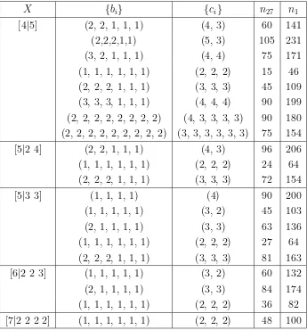
X {bi} {ci} n27 n1 [4|5] (2, 2, 1, 1, 1) (4, 3) 60 141
(2,2,2,1,1) (5, 3) 105 231 (3, 2, 1, 1, 1) (4, 4) 75 171 (1, 1, 1, 1, 1, 1) (2, 2, 2) 15 46 (2, 2, 2, 1, 1, 1) (3, 3, 3) 45 109 (3, 3, 3, 1, 1, 1) (4, 4, 4) 90 199 (2, 2, 2, 2, 2, 2, 2, 2) (4, 3, 3, 3, 3) 90 180 (2, 2, 2, 2, 2, 2, 2, 2, 2) (3, 3, 3, 3, 3, 3) 75 154 [5|2 4] (2, 2, 1, 1, 1) (4, 3) 96 206 (1, 1, 1, 1, 1, 1) (2, 2, 2) 24 64 (2, 2, 2, 1, 1, 1) (3, 3, 3) 72 154
[5|3 3] (1, 1, 1, 1) (4) 90 200
[image:22.612.125.470.35.405.2](1, 1, 1, 1, 1) (3, 2) 45 103 (2, 1, 1, 1, 1) (3, 3) 63 136 (1, 1, 1, 1, 1, 1) (2, 2, 2) 27 64 (2, 2, 2, 1, 1, 1) (3, 3, 3) 81 163 [6|2 2 3] (1, 1, 1, 1, 1) (3, 2) 60 132 (2, 1, 1, 1, 1) (3, 3) 84 174 (1, 1, 1, 1, 1, 1) (2, 2, 2) 36 82 [7|2 2 2 2] (1, 1, 1, 1, 1, 1) (2, 2, 2) 48 100
Table 9: The particle content for the E6-GUT theories arising from our classification of stable, positive SU(3) monad bundles V on the Calabi-Yau threefold X. The number n27 of anti-generations vanishes.
of anti-generations vanishes and the number of generations can be computed from the index, so that
n16=h1(X, V) =−ind(V), n16= 0 . (54)
Thus, for the rank 4 bundles in Tables 4–8, the (negative) of the right-most column gives the number of 16representations.
Next, we need to compute the Higgs content which is given byn10=h1(X,∧2V). It
can be shown in general that for generic mapsg:B →C the number of10 representa-tions always vanishes, that is
n10= 0. (55)
Finally, we need to compute the numbern1of SO(10) singlets which is easily obtained
from Eq. (53). The results for the spectrum from rank 4 bundles are summarized in Table 10.
A vanishing number,n10, of Higgs particles is not desirable from a particle physics
viewpoint. One might, therefore, wonder whether more specific choices of the map g
in (18) could produce a non-zero value for n10. This problem has been encountered
in Ref. [5, 24, 6] where the spectrum of compactification was shown to depend on the region of moduli space. Specifically, it was shown that the spectrum takes a generic form with possible enhancements in special regions of the moduli space; this was dubbed the “jumping phenomenon” in [24, 6].
To see that a similar phenomenon can arise for monad bundles, let is consider the following SU(4) bundle on the quintic, [4|5].
0→V → O⊕2
X (2)⊕ O ⊕4 X (1)
g
−→ O⊕2
X (4)→0. (56)
This bundle and its particle content for a generic map g is given in the first line of Table 10. Now we explicitly define the map gby
g= 4x
2
3 9x20+x22 8x23 2x33 4x31 9x31 x2
0+ 10x 2
2 x
2
1 9x 3 2 7x
3 3 9x
3 1+x
3 2 x
3 1+ 7x
3 4
!
. (57)
where x0, . . . , x4 are the homogeneous coordinates of P4. This choice for g is no longer
completely generic, although the sequence (56) is still exact. Following the steps in Appendix A.4, we can use Macaulay to calculate the spectrum for this case. We find
n16= 90, n16= 0, n10= 13 , n1 = 277. (58)
This is identical to the generic result in Table 10, except for the number of 10 represen-tations which has changed from 0 to 13.
4.4
SU
(5)-GUT Theories
Finally, we should consider SU(5) GUT theories which originate from rank 5 bundles with structure group SU(5). To demonstrate their stability from Hoppe’s criterion we have to show that H0(X,ΛpV∗
) for p= 1,2,3,4 vanish. Forp= 1,2,4 this has already been accomplished in Section 3.3, so it remains to deal with the case p= 3.
Unfortunately, for p = 3 the long exterior power sequences (34) together with Ko-daira vanishing are not quite sufficient to prove thatH0(X,Λ3V∗
) = 0. Indeed, writing down (33) for p= 3 we find
0→S3C∗
→S2C∗
⊗B∗
→K1 →0 ,
0→K1 →C∗⊗ ∧2B∗→K2 →0, (59)
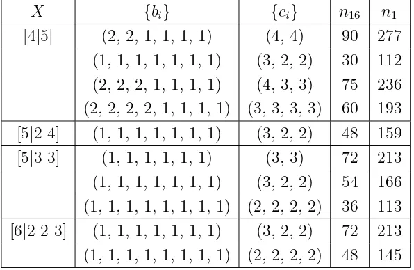
X {bi} {ci} n16 n1 [4|5] (2, 2, 1, 1, 1, 1) (4, 4) 90 277
[image:24.612.149.447.37.231.2](1, 1, 1, 1, 1, 1, 1) (3, 2, 2) 30 112 (2, 2, 2, 1, 1, 1, 1) (4, 3, 3) 75 236 (2, 2, 2, 2, 1, 1, 1, 1) (3, 3, 3, 3) 60 193 [5|2 4] (1, 1, 1, 1, 1, 1, 1) (3, 2, 2) 48 159 [5|3 3] (1, 1, 1, 1, 1, 1) (3, 3) 72 213 (1, 1, 1, 1, 1, 1, 1) (3, 2, 2) 54 166 (1, 1, 1, 1, 1, 1, 1, 1) (2, 2, 2, 2) 36 113 [6|2 2 3] (1, 1, 1, 1, 1, 1, 1) (3, 2, 2) 72 213 (1, 1, 1, 1, 1, 1, 1, 1) (2, 2, 2, 2) 48 145
Table 10: The particle content for the SO(10)-GUT theories arising from our classification of stable, positive, SU(4) monad bundles V on the Calabi-Yau threefold X. The number n16 of anti-generations vanishes. The number n10 vanishes for generic choices of the map g in the monad sequence (18), but can be made non-vanishing with particular choices of g.
Now, using the 3 intertwined long exact sequences in cohomology induced by the above 3 sequences, together with Kodaira vanishing for the negative bundles formed from the symmetric and anti-symmetric powers of B∗ and C∗, we can only conclude that
H0(X,∧3V∗
)≃H2(X, K1) . (60)
We will now show that the stability proof can be completed by applying Koszul resolu-tions to our rank 5 bundles. This technique makes explicit use of the embedding in the ambient spaceA=Pmand its complexity grows with the number of co-dimensions of the
Calabi-Yau manifold X inA. We, therefore, start with the quintic, X= [4|5], the only co-dimension one example among the five Calabi-Yau manifolds under consideration, before we proceed to the more complicated examples.
4.4.1 Stability for Rank 5 Bundles on the Quintic
For the quintic, the normal bundle is simply given by N = O(5) and the Koszul se-quence (40), applied to W = Λ3V∗
, explicitly reads 0→ N∗
⊗ ∧3V∗
→ ∧3V∗
→ ∧3 V∗
→0. (61)
From this, we have the long exact sequence in cohomology, 0→H0(A,N∗
⊗ ∧3V∗
)→H0(A,∧3V∗
)→H0(X,∧3V∗
)→H1(A,N∗
⊗ ∧3V∗
)→...
(62) Thus, if we knew H0(A,∧3V∗
) and H1(A, N∗
⊗ ∧3V∗
), we could hope to determine
writing down the ambient space version of the exterior power sequences (59) tensored by N∗
.
0 → N∗
⊗S3C∗ h
→ N∗
⊗S2C∗
⊗ B∗
→ K1→0 ,
0 → N∗
⊗ K1 → N∗⊗ C∗⊗ ∧2B∗→ K2 →0 , (63)
0 → K2 → N∗⊗ ∧3B∗ → N∗⊗ ∧3V∗→0 .
Since B∗
, C∗
and N∗
are all negative bundles, it follows that H0(A,∧3V∗
) = 0 and
h1(A,N∗⊗ ∧3V∗
) =h3(A,K
1) = ker(h′), whereh′:H4(A,N∗⊗S3C∗)→H4(A,N∗⊗ S2C∗
⊗ B∗
) is the map induced from h above. Now, we note that since the ranks of the maps in the defining monads were chosen, by construction, to be maximal rank, it follows that the induced maphin the exterior power sequence is also maximal rank. To proceed further, we finally observe that for any generic, maximal rank map h:U → W between two ambient space bundles U and W the induced map ˜h : H0(A,U) → H0(A,W) is
also maximal rank (see Appendix B.2). Since the sequences above are all defined over the ambient space andh is maximal rank, it follows from the above argument thath′
is maximal rank and ker(h′
) = 0. Therefore,
h1(A,N∗
⊗ ∧3V∗
) = 0. (64)
Thus, returning to (62), we find that H0(X,∧3V∗
) = 0 and by Hoppe’s criterion, all generic, positive SU(5)bundles are stable on the quintic.
4.4.2 The Co-dimension 2 and 3 Manifolds
The stability proof for our remaining rank 5 bundles is similar in approach, but slightly more lengthy than that given in the previous subsection. In the interests of space, we will only give an overview of it here. We recall from Subsection 4.1 that the remaining Calabi-Yau manifolds with rank 5 bundles are defined by two and three constraints in
P5 and P6 respectively. We first look at the co-dimension two case.
For co-dimension two, the normal bundle takes the form N =O(q1)⊕ O(q2) with q1, q2 >0. This time the Koszul sequence (40) is no longer short-exact, but reads
0→ ∧2N∗
⊗ ∧3V∗
→ N∗
⊗ ∧3V∗
→ ∧3V∗ ρ
→ ∧3V∗
→0 . (65)
It can be split into two short exact sequences,
0 → ∧2N∗
⊗ ∧3V∗
→ N∗
⊗ ∧3V∗
→ K →0 ,
0 → K → ∧3V∗ ρ
→ ∧3 V∗
→0 . (66)
From the long cohomology sequences of these two resolutions, we find thatH0(X,∧3V∗
)≃
H2(A,∧2N∗
⊗ ∧3V∗
) (since H0(A,∧3V∗
) = H0(A,N∗
⊗ ∧3V∗
written over P5 yields,
0 → ∧2N∗
⊗S3C∗ h
→ ∧2N∗
⊗S2C∗
⊗ B∗
→ K1→0 ,
0 → K1 → ∧2N∗⊗ C∗⊗ ∧2B∗→ K2→0 ,
0 → K2 → ∧2N∗⊗ ∧3B∗ → ∧2N∗⊗ ∧3V∗→0 . (67)
Once again, we find that H2(A,∧2N∗ ⊗ ∧3V∗) ≃ H4(A,K
1) and h4(A,K1) = ker(h′)
whereh′
:H5(A,∧2N∗⊗ S3C∗
)→ H5(A,∧2N∗⊗
S2C∗⊗ B∗
). As before, it follows from our definition of the monad that h′
is maximal rank and ker(h′
) = 0. Therefore, all positive rank 5 bundles on the manifolds [5|2 4] and [5|3 3] are stable.
With this analysis complete, we are left with only one rank 5 bundle on the co-dimension 3 manifold, [6|2 2 3], to consider. In this case, we could directly apply the Koszul resolution techniques as above, with a normal bundle,N =O(2)⊕ O(2)⊕ O(3), and higher antisymmetric powers in the Koszul resolution (40). Note, however, that in this case we are not assured that the dual sequence (22) is well defined on the ambient space, since the numeric criteria in Theorem 3.2 are not satisfied onP6. However, we can
still compute the cohomology of the relevant sheaves onP6. The calculation is lengthy,
but straightforward.
It is worth noting that there is an alternative approach to this case. Instead of viewing the Koszul resolution as describing the restriction of objects on Pm to the
Calabi-Yau, we may view X= [6|2 2 3] as a sub-variety in the 4-fold Y = [6|2 2]. Then we may apply the Koszul techniques exactly as before, viewing the normal bundle to the Calabi-Yau as a line bundle, OY(3) in [6|2 2]. The analysis then reduces to that
described for the co-dimension 1 case (61) (that is, that of the rank 5 bundles on the quintic). A straightforward calculation shows that H0(X,∧3V∗
) = 0 and the final rank 5 bundle is stable.
4.4.3 Particle Content
We have shown, using the Koszul sequence, that all positive rank 5 bundles in our classification are stable. Let us now analyze their particle spectrum. From Table 2, we need to compute n10 = h1(X, V), n10 = h
1(X, V∗
) = h2(X, V), n
5 = h1(X,∧2V), n5 = h1(X,∧2V
∗
) = h2(X,∧2V), and n
1 = h1(X, V ⊗V∗). As for rank 4 and 5
bundles, we have h0(X, V) = h3(X, V) = 0 from stability and h2(X, V) = 2 from the
sequence (30). Consequently, we find
n10=h1(X, V) =−ind(V), n10= 0 . (68)
As before, we have no anti-generations and the (negative) of the index, listed in right-most column of Tables 4–7, gives the number n10 for all rank 5 bundles. We include
these in Table 11 for reference.
Next, we need to compute the H1(X,∧2V) and H2(X,∧2V). From the above
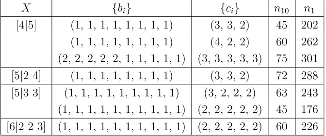
X {bi} {ci} n10 n1 [4|5] (1, 1, 1, 1, 1, 1, 1, 1) (3, 3, 2) 45 202
[image:27.612.130.466.37.178.2](1, 1, 1, 1, 1, 1, 1, 1) (4, 2, 2) 60 262 (2, 2, 2, 2, 2, 1, 1, 1, 1, 1) (3, 3, 3, 3, 3) 75 301 [5|2 4] (1, 1, 1, 1, 1, 1, 1, 1) (3, 3, 2) 72 288 [5|3 3] (1, 1, 1, 1, 1, 1, 1, 1, 1) (3, 2, 2, 2) 63 243 (1, 1, 1, 1, 1, 1, 1, 1, 1, 1) (2, 2, 2, 2, 2) 45 176 [6|2 2 3] (1, 1, 1, 1, 1, 1, 1, 1, 1, 1) (2, 2, 2, 2, 2) 60 226
Table 11: The particle content for the SU(5)-GUT theories arising from our classification of stable, positive, SU(5) monad bundles V on the Calabi-Yau threefold X. The number of anti-generations, n10, vanishes. Further, n5 = n10. Moreover, n5 = 0 for generic choices of the mapg in Eq. (18), and can be made non-vanishing in special regions of moduli space.
H3(X,∧2V) both vanish (recall that we have already shown explicitly thatH0(X,∧2V∗
) =
H3(X,∧2V) vanishes). Therefore, applying the index theorem (4) to Λ2V we have
−h1(X,∧2V) +h2(X, X,∧2V) = ind(∧2V) = 1
2
Z
X
c3(∧2V) . (69)
For SU(n) bundles one has (see Eq. (339) of Ref. [6]),
c3(∧2V) = (n−4)c3(V) . (70)
Hence, combining (69) and (70), we find the relation
−n5+n5 = ind(V) =−n10 . (71)
We still need to compute one of the numbers n5 and n5. Macaulay [23] can very easily
calculate n5=h1(X,∧2V∗
) =h2(X,∧2V). It turns out that
n5 = 0 (72)
for all rank 5 bundles and generic choices 4 of the mapg. From Eq. (71) this implies
n5 =n10, (73)
and, hence, the complete spectrum is determined by n10 and n1. We have listed these
numbers in Table 11.
5
Conclusion
In this paper, we have presented a classification of positive SU(n) monad bundles on the five Calabi-Yau manifolds defined by complete intersections in a single projective space.
4
We have required that these bundles can be incorporated into a consistent heterotic compactification where the heterotic anomaly cancellation condition can be satisfied by including an appropriately wrapped five-brane. In addition, we have imposed two “physical” conditions, namely that the rank of bundle be n= 3,4,5 (in order to obtain a suitable grand unification group) and that the index of the bundle (that is, the chiral asymmetry) is a non-zero multiple of three. Given these conditions, we found 37 bundles on the five Calabi-Yau manifolds in question, 20 for rank 3, 10 for rank 4 and 7 for rank 5. Using a simple criterion due to Hoppe, we have shown that all these bundles are stable and, hence, lead to supersymmetric compactifications. We have also computed the full particle spectrum for all 37 cases, including the number of gauge singlets. A generic feature of all our bundles is that the number of anti-generations vanishes.
These results show that a combination of analytic computations and computer al-gebra can be used to analyze a class of models algorithmically. In particular, we have seen that the notoriously difficult problem of proving stability can be addressed sys-tematically and that the full particle spectra can be obtained for all cases. Although the final number of models is still relatively small we expect that these methods can be extended to much larger classes of Calabi-Yau manifolds, such as complete intersections in products of projective spaces and in weighted projective spaces. Such a large-scale analysis which is currently underway [9] will lead to a substantial number of examples with broadly the right physical properties. This class of models can then be used to implement more detailed particle physics requirements and to systematically search for examples close to the standard model.
Acknowledgments
The authors would like to expression our sincere gratitude to Maria Brambilla, Philip Candelas, Dan Grayson, Tristan H¨ubsch, Lionel Mason, Balasz Szendroi and Andreas Wisskirchen for helpful discussions. Our special thanks go to Adrian Langer whose help with some of the relevant mathematical problems was invaluable. L. A. thanks the US NSF and the Rhodes Foundation for support. Y.-H. H is indebted to the FitzJames Fellowship of Merton College, Oxford. A. L. is supported by the EC 6th Framework Programme MRTN-CT-2004-503369.
A
Monads, Sheaf Cohomology and
Computa-tional Algebraic Geometry
phenomenology in [26] and the reader is referred to tutorials in these papers as well for a quick introduction.
A.1
The Sheaf-Module Correspondence
Since we are concerned with compact manifolds, we will focus on projective varieties in
Pm. A projective algebraic variety is the zero locus of a set of homogeneous polynomials
in Pm with coordinates [x
0 : x1 : . . . : xm]. In the language of commutative algebra,
projective varieties correspond to homogeneous ideals, I, in the polynomial ring RPn =
C[x0, . . . , xm]. An ideal I ⊂RPn, associated to a variety, is generated by the defining
polynomials of the variety and consists of all polynomials which vanish on this variety. The quotient ring A=RPn/I is called thecoordinate ringof the variety.
In general, a ring R is calledgraded if
R=M
i∈Z
Ri, such thatri∈Ri, rj ∈Rj ⇒rirj ∈Ri+j .
For the polynomial ring RPn theRi consists of the homogeneous polynomials of degree
i. In analogy to vector spaces over a field, one can introduce R-modules M over the ring R. In practice, one can think ofM as consisting of vectors with polynomial entries with R acting by polynomial multiplication. A module is called graded if
M =M
i∈Z
Mi, such that ri ∈Ri, mj ∈Mj ⇒rimj ∈Mi+j .
The graded ring Ris itself a graded R-module, M(R). Similarly, an idealI in a graded ring R is a graded R-module and a submodule of M(R). Another important example of a graded Rmodule isR(k) which denotes the ringRwith degrees shifted by −k. For example, x2y ∈R
Pn is of degree 3, but seen as an element of the module R
Pn(−2), its
degree is 3 + 2 = 5.
Sheafs over a (projective) variety can also be described as a module by virtue of the sheaf-module correspondence. Given the graded ring R and a finitely generated graded R-module M, one defines an associated sheaf Mf as follows. On an open set
Ug, given by the complement of the zero locus of g ∈ R, the sections over Ug are
f
M(Ug) = {m/gn|m ∈ M ,degree(m) = degree(gn)}. On Pm, this looks concretely as
follows. A sufficiently fine open cover of Pm is provided by U
xi, the open sets where
xi6= 0. Let us first consider the moduleM(RPn), that is, the ringR
Pn seen as a module.
ThenM^(RPn)(Ux
i) ={f /x
m
i , f homogeneous of degree n}and, hence,
^
M(RPn) =OPm,
where OPm is the trivial sheaf onPn. Similarly, for the modulesR
Pn(k) one has
OPm(k)≃R^Pn(k) .
For projective varieties X ⊂Pm and associated ideal I, the story is similar. Now, one
needs to consider the graded modules over the coordinate ring A=R/I. In particular, for line bundles OX(k) on X one has
![Table 5: Positive monad bundles on [5|2 4].](https://thumb-us.123doks.com/thumbv2/123dok_us/1637385.117089/18.612.106.489.87.368/table-positive-monad-bundles-on.webp)
![Table 6: Positive monad bundles on [5|3 3].](https://thumb-us.123doks.com/thumbv2/123dok_us/1637385.117089/19.612.155.444.608.645/table-positive-monad-bundles-on.webp)