Opportunities and constraints in the use of simulation on low cost ARM-based computers

Opportunities and constraints in the use of simulation on low cost

ARM-based computers

Dr Jon W Hand1

1 _{Energy Systems Research Unit, University of Strathclyde, Glasgow, Scotland}

Abstract

The whole-building simulation community has habitually demanded greater computational resources and developers and researchers have responded with a myriad of approaches to address this demand. How-ever, much of the work of creating and evolving models takes a frac-tion of the available computafrac-tional power.

This paper considers the deployment of simulation at the other ex-treme of computational cost e.g. ARM based products such as the Raspberry Pi and the BeagleBone Black. This paper reports on the porting of the ESP-r whole-building suite to ARM. It describes the modifications required to the simulation software as well as to the compilation tool-chain and computing environment to support compi-lation and deployment. It discusses the performance implications of model complexity and adjustments to methodologies required as well as the user reactions. It also describes how research based on tools such as MATLAB can be hosted on these alternative computer plat-forms.

1

Introduction

There is a great deal of buzz in the technical press about a new generation of ultra-low cost computers - in particular the Raspberry Pi targeted at helping students learn programming and supporting 'Maker' projects such as robotics. A number of competing products have emerged to form a lively ecosystem of ARM based single-board computers that typically run a low-resource version of Linux or Android with costs in the region of 35-50 US Dollars. ARM chips are most often seen in tablets and cell phones because of their very low energy de-mands.

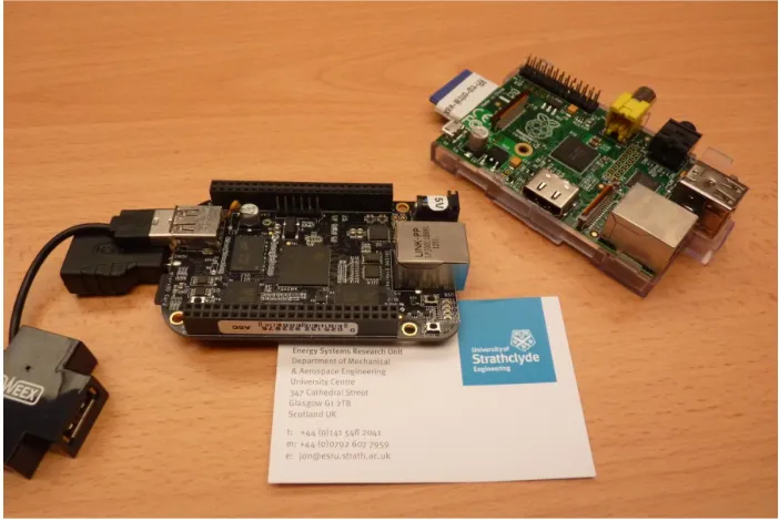
The evolution in this market is fast-paced with multi-core processors and better specifications being announced on a weekly basis. This project has used the Raspberry Pi (based on an old-er ARM chip) and the BeagleBone Black (BBB representing a newold-er genold-eration of ARM chip). In Figure 1 the BBB is on the left and the Raspberry is on the right with a business card for scale.

Figure 1: ARM based computers

One driver for the author was the hassle of setting up computers for training workshops and for student projects. Inevitably some participants experience hardware issues which disrupt the smooth flow of workshops. Ensuring alternative computers are available is a logistics is-sue that might be much more tractable if one could bring along a half dozen business-card sized computers which were already proven to work and only required local monitors and keyboards. Most of our training workshops and student projects make use of models which are focused on specific tasks or which are quick to build. The first step would be to assess whether these alternative computers could host workshop models and support the tasks typi-cally included in workshops. But would this be an acceptable user experience?

A review of simulation based consulting projects carried out in ESRU indicated quite a few which involve models of limited complexity and or which are highly focused. Would it be physically possible to have generated the models and solved the issues involved in these pro-jects? Would the predictions be numerically similar to the more common Intel processor fam-ily? The diversity of consulting models is a good test of the likely boundaries of ARM based simulation.

2

Software adaptations

The first stage of the work involved identification of the similarities and differences with the computing infrastructure typically used with ESP-r and deployed by research and consulting staff. ESP-r runs on a range of computing platforms and operating systems e.g. Linux, Unix, OSX, Windows (either as native applications or via Cygwin environment). It uses the GNU compiler suite (GCC G++ Gfortran) which are available on each of these platforms. ESP-r can be compiled with an X11 interface, a cross-platform GTK interface or a pure-text inter-face for use as a back-end engine or for automation tasks so tests of each interinter-face on ARM would be useful. ESP-r is numerically intensive, but each application is single threaded. Sev-eral of its modules are disk intensive (e.g. an assessment of complex model at one minute build-side timesteps and a one second system side might generate 20GB of files). More in-formation on ESP-r can be found in (Hand 2011) and (ESRU 2013).

in header files. As it happens, the array parameters tend to be constrained because there are few practitioners who can manage projects with more than ~5000 surfaces. Historical de-ployments on Sun Workstations typically involved RAM in the order of 400-500MB while current advise is for 1GB or more. The availability of excess RAM allows performance data written to files to be held in memory buffer which greatly speeds (two orders of magnitude) subsequent data recovery tasks.

Both the Raspberry Pi and the BeagleBone Black have 512MB of RAM. Both reserve some memory for the GPU so available memory reduced. Many ESP-r modules exceed this and demand virtual memory in order to run. ESP-r is comprised of many modules, often running simultaneously, and this increases the demand for virtual memory. RAM is thus a challenge. Both single-board computers make use of SDHC or micro-SDHC cards to hold the operating system and user files with the option of USB-2 supplemental data stores. These devices are slow in comparison to either rotational drives or SSD drives. They typically achieve 12-24 MB/s transfer rates. For disk-bound applications this is a challenge. And these slow data de-vices are also used for virtual memory.

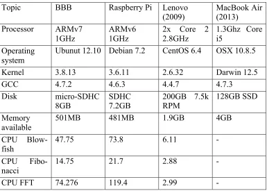
The specifications of the two ARM computers as well as conventional Lenovo workstation (circa 2009) and a laptop (MacBook Air circa 2013) are used for comparison. Timings from HARDINFO reports (smaller numbers are faster in the CPU Blow-fish, Fibonacci and FFT) are shown in Table 1.

Table 1: Computers used in the tests

Topic BBB Raspberry Pi Lenovo

(2009) MacBook Air (2013) Processor ARMv7

1GHz ARMv6 1GHz 2x Core 2 2.8GHz 1.3Ghz Core i5 Operating

system

Ubunut 12.10 Debian 7.2 CentOS 6.4 OSX 10.8.5

Kernel 3.8.13 3.6.11 2.6.32 Darwin 12.5

GCC 4.7.2 4.6.3 4.4.7 4.7.3

Disk micro-SDHC

8GB

SDHC 7.2GB

200GB 7.5k RPM

128GB SSD

Memory available

501MB 481MB 1.9GB 4GB

CPU Blow-fish

47.75 73.8 6.11 -

CPU Fibo-nacci

14.75 21.7 2.88 -

CPU FFT 74.276 119.4 2.99 -

Changes in the compilation tool chain

ESP-r compilation is based on the GNU tool chain and relies on Makefiles and shell scripts to support the build process and setting up databases and example models. Both ARM proces-sors offer these facilities. During setup, dependencies and library locations must be managed. The initial task was to adapt the Install script to detect arm6l and arm7l chip sets and specify paths to libraries and variant names of libraries.

compila-tion proceeded, albeit slowly. Much of the delay was found in the linking phase - it could take longer to link the object files than to generate the object files. The addition of a --reduce-memory-overheads option speeded up the linking process by an order of magnitude and re-duced the need for virtual memory during the linking stage.

Initial tests indicated that smaller ESP-r modules (like the weather analysis tool) were able to run but the simulator and project manager would fail to run due to memory limitations. What was needed was a small footprint version of the header files. A static memory analysis via the forcheck (www.forcheck.nl) tool identified a number of 4 and 5 dimensional arrays that were responsible. Four of the primary header files controlled the level of model complexity for zones, controls, the flow mass flow and CFD domains.

After several iterations the zone footprint which is supported by 512MB RAM is 32 thermal zone, 2000 models surfaces. Each zone and surface polygon could be as complex as the standard version but no more than a dozen layers in each construction would be allowed. In the mass flow domain 40 nodes and components are allowed along with 100 connections. For CFD the gridding was restricted to 14 nodes in each axis and for controls the number of con-trol loops was reduced to 32. The use of alternative headers allowed the compilation to pro-ceed much faster and for multiple modules to run simultaneously.

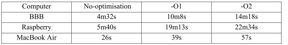
One finding is that armv6l computers (like the Raspberry Pi) are, in general twice as slow in the compilation phase as the armv7l (BBB) newer ARM chip sets. The full compile of ESP-r is shown in the following table. Although a typical build for ESP-r does not invoke compiler optimisations, in the context of lower power computers options for increasing speed are of interest and the tests included ESP-r modules built with the -O1 and -O2 GNU compiler op-tions. These impose considerable penalties in the compilation phrase, particularly for the Raspberry Pi as can be seen in the following table for the stand-alone CFD solver module:

Table 2: Compilation times for dfs module

Computer No-optimisation -O1 -O2

BBB 4m32s 10m8s 14m18s

Raspberry 5m40s 19m13s 22m34s

MacBook Air 26s 39s 57s

Performance issues

One would expect the performance of simulation tools on a thirty Dollar computer is different from that of a 300 or 3000 Dollar computer. However, the computational demand for differ-ent simulation tasks and user interactions is considerable and requires testing.

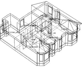
Of interest is the degree to which user controlled options, such as the amount of data to be recorded or the length of the simulation period might be important. To determine general per-formance, tests were carried out for three different ESP-r models. Two are exemplar models used in training exercises and the third was taken from a consulting project involving retrofit options for an1890s traditional stone tenement building.

Figure 2: Cellular_shd model view

Figure 3: Traditional stone tenement for stone_simi_1890.

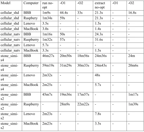
Table 3: run-time performance Model Computer run

no-opt

-O1 -O2 extract no-opt

-O1 -O2

cellular_shd BBB 1m9s 44.4s 33s 21.3s - 16.8s

cellular_shd Raspbery 1m34s 59s - 21.3s - -

cellular_shd Lenovo 3.5s - - 1.5s - -

cellular_shd MacBook 3.0s - - 1.4s - -

cellular_natv BBB 1m16s 50s - 24.3s - -

cellular_natv Raspberry 1m32s 57s - 31.6s - -

cellular_natv Lenovo 5.7s - - - -

cellular_natv MacBook 3.3s - - 1.5s - -

stone_simi-s4

BBB 46m27s 20m50s 18m56s 24m36s - 24m

stone_simi-s4

Raspberry 59m19s 31m29s 30m33s 24m43s - 20m6s

stone_simi-s4

Lenovo 2m32s - - 48s - -

stone_simi-s4

MacBook 2m25s - - 5.7s - -

stone_simi-s2 BBB 45m7s 19m36s 17m57s - - 1m17s

stone_simi-s2

Raspberry - 28m9s 22m22s - - 1m39s

stone_simi-s2

Lenovo 2m23s - - 7.8s - -

stone_simi-s2 MacBook 2m23s - - 3.5s - -

The size of the results stored is important. The ~80MB files associated with the moderate save of predictions took less time to write, was held in buffer and was thus accessed via RAM. The ~700MB results file required an explicit scan and was clearly disk-bound. The use of optimization was also seen to have a significant impact on the time required for as-sessments, and to a lesser degree on the time required to recover performance information.

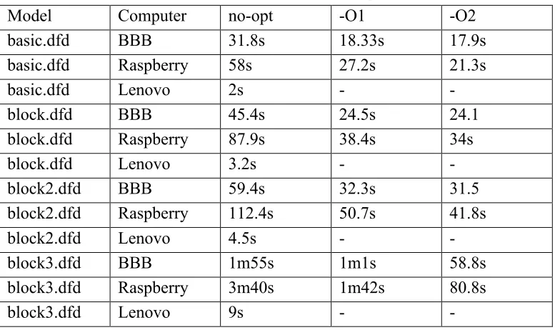
Exploring computational boundariest

• a simple static domain (basic.dfd) which would convergence in ~250 iterations, • a domain (block.dfd) which would tend to converge in ~350 iterations

• a domain (block2.dfd) that would tend to converge in ~450 iterations • a domain (block3.dfd) that would tend to converge in ~850 iterations.

Table 4: CFD solution performance

Model Computer no-opt -O1 -O2

basic.dfd BBB 31.8s 18.33s 17.9s

basic.dfd Raspberry 58s 27.2s 21.3s

basic.dfd Lenovo 2s - -

block.dfd BBB 45.4s 24.5s 24.1

block.dfd Raspberry 87.9s 38.4s 34s

block.dfd Lenovo 3.2s - -

block2.dfd BBB 59.4s 32.3s 31.5

block2.dfd Raspberry 112.4s 50.7s 41.8s

block2.dfd Lenovo 4.5s - -

block3.dfd BBB 1m55s 1m1s 58.8s

block3.dfd Raspberry 3m40s 1m42s 80.8s

block3.dfd Lenovo 9s - -

With minor exceptions the number of iterations required are the same as on standard work-stations and the results are nearly identical. Clearly optimization is worthwhile for these nu-merical calculations and the newer ARM chip was both faster to compile with optimization and provided better performance.

User perceptions

A number of students and researchers have observed the author working on projects and only a few noticed that the work being done via a single-board computer rather than the adjacent workstation. The author observed several users carrying out various tasks on single-board computers that they would normally have done on a standard computer. Where their work involved an existing model this was copied into the ARM computer. Models taken from other Linux and OSX computers were seen to work out-of-the-box. With minimal support users continued to carry out their tasks. Where models were sourced from Windows machines these were converted via standard Windows-to-Linux conversion scripts. When presented with the same style of ESP-r interface as found on Windows they a minimum of support was needed after a five minute introduction to operating system navigation skills. Use of file transfer to port their work back to their standard computer was quickly learned and took only moments. For example, a colleague working on a validation project switched to the BBB for a morning and found the session mostly unremarkable. The standard test for the validation project took a couple of minutes to run between tweaks to the model and checking model details. The col-league was intrigued by the idea that they would not need to mess with their own home com-puter if they could use an ARM single-board comcom-puter for light work.

sta-ble display when connected via HDMI-HDMI monitors or TV sets. In general ESP-r requires limited graphics resources and would not tax a GPU.

Another observation is that ARM computers tend to be sensitive to electrical power quality – they needed their full rated power ~5-8W to work reliably under load. They also can fault when removing USB devices so they require slightly different user habits.

It was found that these single board computers performed well as stand-by computers for ESP-r workshops. When brought into service, users were able to continue with their work and sessions continued at the same pace. Participants essentially forgot what computer was being used.

Tasks involving traversing the command menus in ESP-r applications were not perceived as an issue by any of the workshop participants or test subjects. There was no noticeable lag in response and participants were able to carry out their tasks in selecting entities, altering focus within the model and carrying out editing tasks.

When users were allowed to use their preferred interface little or no support was required. The X11 interface of ESP-r was marginally faster, especially when compiled with optimization. For simple models rotating the wire-frame view was no different than a conventional work-station. For models at the limit of complexity there was a couple of seconds delay in re-drawing. This would tend to indicate that for projects within the complexity limits of the de-vices, model development and testing tasks could be carried out with very little change in user productivity. Automation that would be regularly applied by simulators can also be deployed but might need to be tweaked to limit the number of applications simultaneously active. The 1-2 minute lag needed to shift models to another computer for production work may or may not be acceptable.

Ancillary tasks

Users of simulation also often make use of other tools to support their work. For example, control engineers deploy MATLAB scripts and a particularly useful niche for small comput-ers would be to combine data acquisition and data processing for control applications.

Initially it was though that a subset of MATLAB functionality could be deployed via MATLAB Coder. Simulink, which is often associated with MATLAB can run on ARM but costs $6500 which was outwith the bounds of this study. MATLAB itself has not been ported to ARM, its native version is memory hungry. However, there is an open-source alternative named Octave (www.gnu.org/software/octave) which has. Installing Octave on ARM is the same as on any other other Linux computer and the graphical interface to it was instantly rec-ognizable and usable with no training.

Figure 4: Diagram of the control logic

Figure 5: Temperatures over two days.

The researcher judged that run-time was not an issue for a model of this complexity and he might consider using Octave with more complex models. The only changes required to the script were to comment out some reporting of variables (a slightly different syntax is needed). The second test involved a research project which used Blade Element Momentum Theory (BEMT) for predicting the performance of a turbine (wind or tidal). BEMT combines the the-ory that all energy extracted by a turbine in a free-stream flow comes from the total change in momentum of the fluid, with the theory that a 3D blade can be thought of as a series of ele-mental sections (of non-differential length), over which the fluid dynamics can be considered as 2D. The theory is widely used, and the derivation of the relevant equations can be found in such texts as the Wind Energy Handbook (Burton 2001) and Aerodynamics of Wind Turbines (Hansen 2008).

The code used in this study had 8 blade elements and assessed the performance over 10 flow conditions. Upon successful convergence, the code then produces a graph, as shown in Figure 6, which displays the predicted performance of the turbine. This BEMT code was produced in MATLAB and runs successfully, in a matter of milliseconds, on a desktop computer. When transferred to OCTAVE, convergence was achieved and the results were displayed in a matter of seconds.

Figure 6: BEMT display of turbine performance

Again, the MATLAB script ran without change but the graph produced had a few artifacts that would have required minor changes in syntax. Although this is not a definitive, Octave on ARM appears to have some degree of applicability.

Control-related tasks

A decade ago the author was involved in a project with Honeywell which ran ESP-r every 5 minutes to feed into a LABVIEW controller (Clarke et.al. 2002). The replacement of algo-rithm-based building energy management with near-real-time simulation continues to be of interest. In the event, these single-board computers have many additional I/O ports for at-tachment to motor controls, sensors and have been deployed in robotics and in projects requir-ing digital controls. Work in ESRU has used these srequir-ingle board computers as data collection and data transformation hubs with wireless sensors (Clarke et.al 2014). Only a fraction of the computational resource was needed to process six second temperature, humidity, light level, movement and audio signals from ~25 low cost remote sensors and thus there are resources available for building simulation tasks running on the processor.

The single-board computers under test are more powerful than those used in the 2002 study and thus it should be possible in the future to deploy these low cost single-board computers in the field to acquire data, feed this to simulation-based BEM (assuming constrained model complexity) and then output control signals. Currently, ESRU is investigating how to adapt the 2002 logic for future deployments.

3

Conclusions

tech-niques for porting legacy software onto the ARM platform. It has also explored, probably for the first time, the deployment of a full dynamic simulation suite to what many people consider to be computers suitable for hobby use and teaching aids in schools. The same claim is likely for running transient 3D CFD assessments on these low power computers.

From the tests it seems like constrained models on ARM computers can run assessments with-in the demands with-in-time control deployments. In other work the author has used Raspberry Pi as data acquisition hub and processor for ultra-low cost wireless sensors and thus it should be possible to host both facilities on these computers.

Use of ARM computers in formal teaching has gotten considerable push-back from col-leagues. The author observed a range of tasks by novices as well as seasoned users with no fatalities (machines or users). Indeed users mostly forgot what computer architecture was be-ing used. It remains to be seen the attrition rate if deployed at a large scale or on models con-sistently at the upper range of complexity. Course work tends to be done on Lab computers with only a few individuals choosing to setup simulation their own computers. After experi-encing single-board computers they were viewed as an alternative to enabling dual-boot of their own laptop by some, but not all participants.

University masters and PhD students have also been observed undertaking a range of tasks with little or no hindrance. Some commented that they would be interested in deploying sin-gle-board computers within simulation-based experiments. Again, whether they would choose such computers is left for a future study.

Certainly there comes a point when computational power is required or model complexity grows to the limits of these low power devices. It has been seen that shifting models between computing platforms is generally not an issue and was a quickly learned task. For those who need to match simulation with third party tools it has been seen that Octave can be used on single-board computers as an alternative to deploying MATLAB.

Optimization was seen to improve interface response as well as numerical tasks and the gen-eral recommendation would be to compile with –O1 optimization for gengen-eral deployment. It is also worth noting that some ARM based single-board computers have on-board NAND memory and do not rely on external SDHC cards. Informal testing indicates that some of the disk access speed issues are addressed. Some vendors also support SATA interfaces and this should allow disk access in line with that of standard computers although this has not be test-ed. Also on single-board computers with 1GB of RAM both the compilation and model com-plexity issues are less stringent.

Lastly, it was not possible to test deployment of ESP-r on ARM based tablets running An-droid. There are several limitations that might apply - ESP-r interfaces can scale down to 800 x 600 resolution displays but both text and wire-frame images are difficult to read. There is no concept in ESP-r that keyboard input might not be available. It is not yet proven that ESP-r can be compiled to run natively on an ARM tablet although both the Raspberry Pi and Bea-glebone Black can boot to Android. If it were possible, one might use this for quick access to model details and reports on-site as well as for targeted editing of model details as one might deploy a laptop but the assumption of keyboard and mouse availability would need to be dealt with. However, it is currently possible to use a tablet as a remote display for ESP-r running on another computer just as it is with any other device that supports remote login and an X11 display server.

4

Acknowledgements

5

References

Beausoleil-Morrison, I., 2000, The adaptive coupling of heaat and airflow modelling within dynamic whole-building simulation, Glasgow, University of Strathclyde.

Burton T et.al, 2001. Wind energy handbook 2001. Available:

http://eu.wiley.com/WileyCDA/WileyTitle/productCd-0470699752.html. Accessed January 2014.

Clarke J A, Cockroft J, Conner S, Hand J W . Kelly N J, Moore R, O'Brien T and Strachan P (2002) Simulation-assisted control in building energy management systems, Energy and Buildings, V34(9), pp933-40.

Clarke J A, Hand J W, Kim J M, Samuel A, Wu D, Royapoor M, Roskily T, Ladha C, Ladha K, Olivier P. Pervasive sensing as a mechanism for the effective control of CHP plant in commercial buildings. To be presented at Building Simulation and Optimization, London, 2014.

ESRU, 2013. Publications page. Available at: http://www.strath.ac.uk/esru/ and http://www.esru.strath.ac.uk/publications.htm [Accessed January, 2014]. Hand, J., 2011. Strategies for Deploying Virtual Representations of the Built

Environ-ment aka The ESP-r Cookbook, Glasgow Scotland: University of Strathclyde. Hansen, M., 2008. Aerodynamics of wind turbines, 2008. Available: