A numerical study into the effects of turbulent flows around full-scale buildings

      

City, University of London Institutional Repository

Citation

:

Basara, B. (1993). A numerical study into the effects of turbulent flows around full-scale buildings. (Unpublished Doctoral thesis, City University London)

This is the accepted version of the paper.

This version of the publication may differ from the final published

version.

Permanent repository link:

http://openaccess.city.ac.uk/8267/

Link to published version

:

Copyright and reuse:

City Research Online aims to make research

outputs of City, University of London available to a wider audience.

Copyright and Moral Rights remain with the author(s) and/or copyright

holders. URLs from City Research Online may be freely distributed and

linked to.

City Research Online: http://openaccess.city.ac.uk/ [email protected]

A NUMERICAL STUDY INTO THE EFFECTS

OF TURBULENT FLOWS AROUND

FULL-SCALE BUILDINGS

Branislav Basara B.Sc. (Eng.)

Thesis submitted for the degree of Doctor of Philosophy

in the School of Engineering City University

Hydraulics Division

Department of Civil Engineering City University

Northampton Square

Abstract

This thesis describes the development and application of a numerical

pre-dictive procedure for turbilent flows around full-scale buildings.

Two different turbulence models were considered: a complete

Reynolds-stress model with two alternative proposals for the pressure-strain

cor-relations and a k-E model used in conjunction with both linear and

non-linear stress-strain relationships.

The governing differential equations were discretized using finite-volume

techniques and a co-located variable-storage arrangement. A multigrid

method was introduced and was found to reduce the computational time

by nearly a factor of ten. Both the Reynolds-stress transport model

and the non-linear k-€ model were implemented in a form suitable for

use with body-fitted coordinates on a co-located grid. When using the

Reynolds-stress models, a number of techniques were utilized to stabilize

the solution process and attain rapid convergence.

The atmospheric boundary layer at inlet to the computation domain,

traditionally specified from empirical correlations, was simulated here

using a full Reynolds-stress model in conjunction with a marching

inte-gration procedure. Due account was taken of the terrain roughness which

matched that for the full-scale tests. The outcome of those simulations

consisted of profiles of mean velocity and turbulence quantities that were

self sustaining and in close accord with the few full-scale measurements

available.

The turbulence models' performance was assessed first through detailed

comparisons with various benchmark flows including the backward-facing

step in both straight and divergent channel, the two-dimensional rib, the

circular cylinder and the three-dimensional cube. Detailed model

verifi-cation was then carried out by comparisons with full-scale measurements

on various structures including a single-span low-rise building, a

semi-cylindrical greenhouse and a multi-span glasshouse. It was found that

the Reynolds-stress models consistently produced more accurate

simula-tions than the

k-E

models. Moreover, it was demonstrated that a recently

proposed model for the pressure-strain correlations yields very

satisfac-tory results without the use of wall-reflection terms.

Acknowledgements

I am very grateful to my Supervisor, Dr B.A.Younis, for his continuos

interest, guidance, encouragement and support during this study.

I wish to thank Prof I. Demirdzic, who made arrangements for my study

at City University and whose helpful advices I greatly appreciate.

I wish also to thank Prof M. Ivanovic, who introduced me to

computa-tional fluid dynamics.

Thanks to my colleagues Dr D. Cokijat, Mr Viado Przulj and Mr Jakirlic

Suad for their support, interest and helpful comments, which are greatly

appreciated.

I acknowledge the financial assistance provided by Agriculture and Food

Research Council - Engineering Institute, Silsoe (grant LRG 169).

Contents

PAGE

Abstract

₁

Acknowledgements

₁₁

Contents

₁₁₁

Nomenclature

_vi

List of figures

_ix

CHAPTER 1 INTRODUCTION

₁

1.1 Background

1

1.2 The present approach and its justification

4

1.3 Previous related studies

6

1.4 Objectives

8

1.5 Contents of thesis

9

CHAPTER 2 MATHEMATICAL FORMULATION

12

2.1 Introduction

12

2.2 Mean-flow equations

13

2.2 The k-€ model

15

2.4 Reynolds-stress transport modelling

22

2.5 Closure

32

CHAPTER 3 SOLUTION PROCEDURE

33

3.1 Introduction

33

3.2 The discretization procedure

34

3.3 Interpolation practices

41

3.3.1 Central differencing schemes

41

3.3.2 Upwind differencing schemes

42

3.3.3 'Power-law' differencing schemes

43

3.3.4 Linear-upwind differencing schemes

44

3.3.5 Hybrid differencing schemes

45

3.4 Pressure-velocity coupling

46

3.5 Pressure-stress-velocity coupling

49

3.6.1 Inlet boundaries

54

3.6.2 Outlet boundaries

54

3.6.3 ymmetry boundaries

54

3.6.4 Fixed pressure boundaries

55

3.6.5 Wall boundaries

57

3.7 Solution algorithm and convergence criterion

59

3.8 A multigrid method

60

3.8.a Multigrid V cycle

61

3.8.b Coarse-grid equations

62

3.8.c Restriction and extrapolation

63

3.8.d Boundary conditions

65

3.8.1 Solution algorithm

65

3.8.2 Verification tests

68

3.9 Closure

69

CHAPTER 4 PRELIMINARY VERIFICATION OF

COMPUTATIONAL METHOD

73

4.1 Introduction

73

4.2 Backward-facing step

74

4.3 Two-dimensional square rib

77

4.4 Backward-facing step in divergent channel

78

4.5 Circular cylinder

81

4.6 Cube

83

4.7 Closure

86

CHAPTER 5 COMPUTATION OF FULL-SCALE FLOWS

114

5.1 Introduction

114

5.2 Simulation of the atmospheric boundary layer 115

5.2.1 Empirical correlations

117

5.2.2 Reynolds-stress transport modelling

119

5.2.3 Effects of inlet profiles

121

5.3 Results for building FB16

122

5.4 Results for building FB17

129

5.5 Results for building G07

131

5.6 Parametric studies

132

5.6.3

Effects of windbreaks

135

5.7

Simulation of peak loads

136

5.8 Closure

139

CHAPTER 6 CLOSURE 191

6.1

Introduction 191

6.2

Fulfillment of objectives

192

6.3

Recommendations for future work

195

NOMENCLATURE

Symbol

Meaning

Ab

A

a13

C

D, CE

Cf,

Cs

Cp

Cc

C 1 ,

Cc2

C4u

Cl

C2

1-Il

r"

'-'1' '-'2

Dj

E

f

I?

, F1

G,

J

k

L

p

p,

p

Pu

Coefficients in discretized equation

Area

Anisotropy tensor

Coefficients in nonlinear stress-strain relationship

Wall skin-friction coefficient

Coefficient in model for triple correlation

Coefficient of pressige

Coefficient in model for diffusion of e

Coefficient in model for sources of

Co efficient in formulation for eddy-viscosity

Coefficient in model for jj

Coefficient in model for

Coefficients in model for 'j,w

Rate of diffusion Uii term

Main rate of strain tensor

Oldroyd derivative

Logarithmic law constant

Wall-dumping function

Mass flux

Instantaneous and time-averaged value of body forces

Tensor in model for

term

Jacobian of coordinate transformation

Turbulence kinetic energy

Turbulence length scale

Time-averaged value of pressure

Fluctuating value of pressure and also pressure correction

Instantaneous value of pressure

Pe

R

q

q

Re

S i , S2 ,

S3

Sjj

S4

t

Tm1 UT U1,u1 UI

uiuj

V

Vb

vs

U \r, w

U,v,w

u2 ,v2 ,

w2

uv,uw, vw

wii

x, y,

z

xl , x2 ,

x3

Yo

yl , y2 ,

y3

y+

Pecklet number

Production of turbulent kinetic energy

Residual

Dynamic pressure

Diffusive flux

Reynolds number

Coefficients in formulation for design wind speed

Mean strain tensor

Source term of variable

Time

Stress tensor

Friction velocity

Time-averaged and fluctuating velocity

Instantaneous value of velocity

Reynolds-stress tensor

Triple velocity correlation

Volume

Basic wind speed

Design wind speed

Fluctuating velocity components in x, y and z directions

Time-averaged velocity components in x, y and z directions

Normal-stress components in x, y and z directions

Shear-stress components

Mean vorticity tensor

Cartesian coordinates

Coordinates of general system

Ground roughness

Cartesian coordinates

Non-dimensional distance from the wall

Greek Symbols

r 6 61j C 'C l-ilt p p Tk, O ni Tw

ii,1, _{LI,2 , LLw}

Coordinate transformation factor

Diffusivity coefficient

Boundary-layer thickness

Kronecker delta

Dissipation of turbulent kinetic energy

Dissipation rate of UfiiJ

Von Karman constant

Molecular viscosity

Turbulent viscosity

Molecular kinematic viscosity

Turbulent kinematic viscosity

Density

Instantaneous density

Coefficients of turbulent diffusion of k and

Shear-stress tensor

Wall shear-stress

Symbol which denotes any variable

Instantaneous and fluctuated value of variable

Terms in modelled pressure-strain correlations

Abbreviations CFD DNS EKE LES LKE NKE RSM RSMO RS Ml

Computational fluid dynamics

Direct numerical simulation

Irrotational-strain modification of € equation

Large-eddy simulation

Linear k-€ model

Non-linear k-€ model

Reynolds-stress model

Pressure-strain correlations proposed by

Launder, Reece and Rodi (1975)

Pressure-strain correlations proposed by

Page

2

36

38

56

61

64

64

70

70

71

72

88

88

89

90

91

92

93

94

List of Figures

Number Title

1.1 Map of the U.K. showing "basic" wind speed in m\s (British Standards Institution,

1991).

3.1

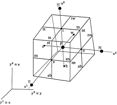
Three-dimensional control volume.

3.2

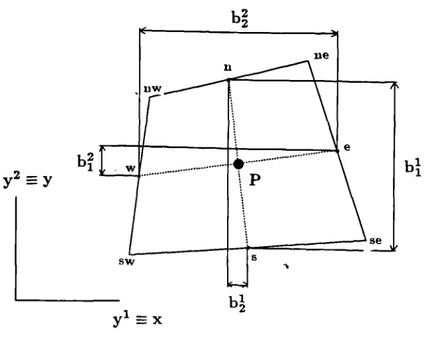
Area projections for two-dimensional control volume.

3.3

Notation for fixed-pressure boundary.

3.4

Multigrid V cycle.

3.5

Restriction-extrapolation scheme.

3.6

Flowchart of solution algorithm.

317

_{Backward-facing step coordinates and geometry.}

3.8

Predicted and measured cross-stream profiles of mean velocity for different grid sizes.

3.9

The nodal absolute relative error on different grids a)

42x17,

b)

82x62

and c)

162x62.

3.10

Multigrid convergence rates for the laminar flow over backward-facing step.

4.1

Backward-facing step coordinates and geometry.

4.2

Backward-facing step. Predicted mean-velocity vectors by LKE.

4.3

Backward-facing step. Predicted streamlines by LKE (a), EKE (b), NKE (c), RSMO (d) and RSM1 (e).

4.4

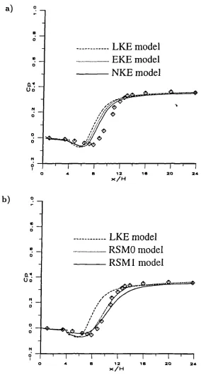
Backward-facing step. Distribution of wall pressure coefficient predicted by LKE, EKE, NKE (a) and LKE,

RSMO, RSM1 (b).

4.5

Backward-facing step. The mean-velocity profiles as obtained by LKE, EKE, NKE (a) and LKE, RSMO,

RSM1 (b).

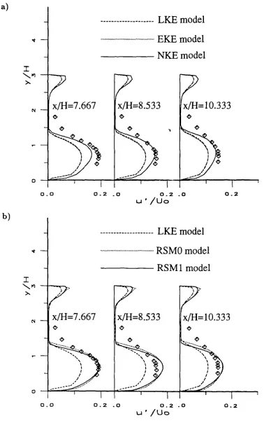
4.6

Backward-facing step. The turbulence intensity profiles as obtained by LKE, EKE, NKE (a) and LKE, RSMO,

RSM1 (b).

4.7

Backward-facing step. The shear stress profiles as obtained by LKE, EKE, NKE (a) and LKE, RSMO, RSM1 (b).

Number Title Page

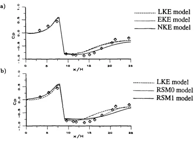
4.9

Two-dimension il rib. Distribution of wall pressure coefficient predicted by LKE, EKE, NKE (a) and LKE,

RSMO, RSM1 (b).

94

4.10

Two-dimensional rib. The mean-velocity profiles as obtained by LKE, EKE, NKE (a) and LKE, RSMO,

RSM1 (b).

95

4.11

Two-dimensional rib. The turbulence intensity profiles as obtained by LKE, EKE, NKE (a) and LKE, RSMO,

RSM1 (b).

96

4.12 Backward-facing step (in divergent channel)

coordinates and geometry

97

4.13

Grid size

185x82:

(a) 0 degree and (b)

6

degree.

97

4.14

Backward-facing step: (a) 0 degree and (b)

6

degree.

Predicted streamlines by RSMO and RSM1.

98

4.15

Backward-facing step: (a) 0 degree and (b)

6

degree. Distribution of wall skin friction coefficient

predicted by RSMO and RSM1.

99

4.16

Backward-facing step: (a) 0 degree and (b)

6

degree. Distribution of wall pressure coefficient predicted by

RSMO and RSM1. 100

4.17

Backward-facing step: (a) 0 degree and (b)

6

degree. The mean-velocity profiles as obtained by RSMO

and RSM1. 101

4.18

Backward-facing step: (a) 0 degree and (b)

6

degree. The shear-stress profiles (iiv) as obtained by RSMO

and RSM1.

102

4.19

Backward-facing step: (a) 0 degree and (b) 6 degree. The normal stress profiles (u2 ) as obtained by RSMO

and RSM1.

103

4.20

Backward-facing step: (a) 0 degree and (b)

6

degree. The normal stress profiles (v2 ) as obtained by RSMO

and RSM1.

104

4.21

The smoothness of grid lines.

82

4.22

Circular cylinder. Grid size 109X67.

105

4.23

Circular cylinder. Distribution of wall pressure

Number Title

Page

4.24

Inflow boundary conditions: velocity U (a),

turbulence kinetic energy k (b) and length scale 1

(c), non-dimensionalized by

UH

and H, measured

in the wind tunnel.

107

4.25

Cube. Computational domain.

107

4.26

Cube. Vertical cross section: 44x28x21 (a), 55x33x28

(b) and 70x48x41 (c).

108

4.27

Cube. Velocity vectors as obtained by measurements a)

and predicted by LKE using the grids A (b) and C (c). 109

4.28

Cube. Velocity vectors predicted by LKE (a), NKE (b)

and EKE (c) (grid C and LUDS scheme).

110

4.29

Cube. Turbulence kinetic energy as obtained by

measurements (a), and predicted by LKE using the

grids A (b) and C (c).

111

4.30

Cube. Turbulence kinetic energy predicted by LKE (a),

NKE (b) and EKE (c) (grid C and LUDS scheme).

112

4.31

Cube. Comparison of surface pressure coefficients at

vertical and horizontal plane (yH/2).

113

5.1

Figure from Hoxey and Richards (1991) showing

measured velocity profiles for the roughness a)

Yo = 40mm and b) yo = 10 mm (N.B:

z above correspond to y in the present notation).

116

5.2

Predicted and measured wall static pressure

coefficients for boundary layer thickness 5=H,

3H, 5H, 7H (FB16).

142

5.3

Predicted and measured wall static pressure

coefficients for S= 55H and 'power-law'

distribution at inlet (FB16).

142

5.4

The physical a) and transformed b) coordinate

system.

120

5.5

The streamwise velocity, turbulence intensity and

dissipation rate profiles as obtained by the Harris

and Deaves correlations and by the Reynolds-stress

model.

5.6

Turbulence intensity profiles as obtained by the

Harris and Deaves correlations and by the

Number Title

Page

5.7

Measured and predicted velocity profile by the

Harris and Deaves correlations and by Reynolds-stress

model. Roughness (a) yo = 10mm and (b) Yo = 40mm.

144

5.8

Predicted wall static pressure coefficient for the

inlet profiles obtained by Harris and Deaves

correlations and by the Reynolds-stress model.

145

5.9

Dimensions of the building FB16 (From Richards, 1989).

146

5.10

Flow visualization on roof of FB16

(From Richards, 1989).

146

5.11

Smoke observations on the roof of the building (a)

and snow tracks in front of the building (b).

147

5.12

FB16. a: Grid 108x100, b: predicted stream lines,

C:

velocity vectors (LKE).

148

5.13

FB16. a: Grid 142x110, b: predicted stream lines, c:

velocity vectors (LKE).

149

5.14

FB16. Distribution of wall pressure coefficient

obtained with the upwind and the power-law

differencing schemes.

150

5.15

FB16. Predicted streamlines for roughness lengths

yo = 0 (a) and for yo = 40mm (b).

151

5.16

FB16. LKE and NKE results for wall static-pressure

distribution.

152

5.17

FB16. Distribution of wall pressure coefficient

predicted by LKE and EKE.

152

5.18

FB16. EKE results for streamlines (a) and velocity

vectors (b).

153

5.19

FB16. Turbulence kinetic energy contours as obtained

by LKE (a) and EKE (b).

154

5.20

FB16. Predicted streamlines by RSMO (a) and RSM1 (b). 155

5.21

FB16. Distribution of wall pressure coefficient

predicted by LKE, RSMO (a), and RSM1 (b).

156

5.22

FB16. Predicted turbulence kinetic energy by

RSMO

and RSM1.

157

5.23

FBI6. Computational domain (height = 300m) covered

Page

159

160

161

162

163

163

164

165

166

167

168

169

170

171

172

173

174

175

176

Number Title

5.24

"New" domain (height = 15m) covered with the grids

37x20 (a), 75x38 (b) and 142x74 (c).

5.25

Predicted streamlines for different grids (a), (b) and (c)

of Fig. 5.24.

5.26

FB16. Grid levels 37x29 (a), 72x56 (b) and 142x110 (c)

used for the multigrid method.

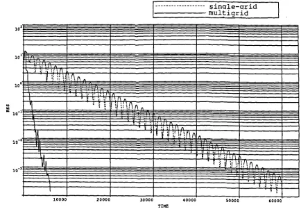
5.27

FB16. The convergence rate obtained with the

multigrid and the single-grid methods.

5.28

Dimensions of Greenhouse FB17 (From Richardson, 1991).

5.29

Grid 216x123 used for FB17.

5.30

FB17. Wall skin-friction coefficient predicted by LKE,

RSMO and RSM1.

5.31

FB17. Predicted streamlines by LKE (a), RSMO (b),

and RSM1 (c).

5.32

FB17. Distribution of wall pressure coefficient

predicted by LKE, RSMO and RSM1 (FB17).

5.33

FB17. Predicted pressure contours by LKE (a) and

RSM1 (b).

5.34

FB17. Predicted turbulence kinetic energy by LKE (a),

RSMO (b) and RSM1 (c).

5.35

Dimensions of multispan structure G07 (From Hoxey

and Moran, 1991)

5.36

G07. Predicted coefficient of wall pressure

distribution.

5.37

G07. Predicted streamlines by EKE (a) and RSM1 (b).

5.38

G07. Predicted turbulence kinetic energy by EKE (a)

and RSM1 (b).

5.39

G07. Grid levels 63x29 (a), 124x56 (b) and 256x110 (c)

used for the multigrid method.

5.40

G07. The convergence rate obtained with the multigrid

and single-grid methods.

5.41

Grid distribution for buildings of same width W but

different heights. H = 3m (a), 4.5m (b), 5.5m (c) and

7m (d).

Number Title

Page

5.43

Predicted average pressure coefficients for buildings

of different heights, on the windward (a), roof

(b) and leeward (c) sides.

177

5.44

Computation domains for the buildings with the same

height and different widths W = 5m (a), 6.7m (b),

8.6m (c) and 10 m (d).

178

5.45

Predicted streamlines for the different widths

W = 5m a), 6.7m b), 8.6m c) and lOm d).

179

5.46

Predicted pressure coefficients for the buildings

with different widths on the windward a), roof b)

and leeward c) side of buUding.

180

5.47

Dimensions of building FB19 (From Robertson, 1989).

Grids for sharp (b) and curved (c) eaves.

181

5.48

Predicted streamlines for sharp eaves a) and curved

eaves b).

182

5.49

Flow visualization around curved eaves. (From

Robertson, 1989).

182

5.50

Velocity vectors for sharp (a) and curved (b) eaves.

183

5.51

Predicted pressure coefficients over roof for sharp

and curved eaves.

183

5.52

Effects of windbreaks. (a) Notation. (b) streamlines

for H=2.18 and X=5m (b).

184

5.53

Predicted average pressure coefficients for the

windward a), roof b) and leeward (c) sides.

185

5.54

Typical records of wind mean velocity and surface

pressure (From Part 2 Code of Practice, 1991)

186

5.55

Unsteady results for the drag coefficient Cd.

186

5.56

Evolution of mean-flow streamlines with time.

187

5.57

Perturbation of velocity at inlet as a function of

time and amplitude.

188

5.58

Predicted pressure coefficient on building roof.

188

5.59

Field measurements of wind velocity at reference

height.

189

Chapter 1

INTRODUCTION

1.1 BACKGROUND

The structural design analysis for full-scale buildings requires knowledge of the pressures exerted on their sides by the turbulent wind flows around them. Those pressures are traditionally obtained from Codes of Practice which utilize the basic definition for the Coefficient of Pressure (Cr) thus:

Ap=Cq (1.1)

The value of C, which is taken to depend on the building shape and on the flow conditions that prevail at the chosen site, is given in tabulated form. q is the dynamic pressure defined as:

q=pV (1.2)

vs =

S1S2 S 3Vb (1.3)

Three empirical correction factors are involved: S 1 which is introduced to take account of local topographic influences (e.g. hilly terrain), S2 which is needed to account for the combined effects of surface roughness, gust duration and the height of the structure and 53 which is related to the design life of the building. Vb is the true (or "basic") wind speed, defined in the UK Code as the 3-second gust speed at lOrn height in open level country likely to be exceeded on average once in 50 years. Its values are reported by the Meteorological Office which employs a wide-spread system of anemographs (continuously-recording wind-speed measuring instruments) to create maps of wind speeds (Fig. 1.1) which are then used for design purposes.

[image:18.595.205.385.318.568.2]

S.-__ --S

Fig. 1.1 Map of the U.K. showing "basic" wind speed in rn/s (British Standards Institution, 1991).

deter-mined from measurements on either full-scale buildings on open sites or on scaled-down models in wind tunnels.

Data collected from full-scale buildings are probably the most appropri-ate for design purposes but they are very scarce and are in the main limited to very few building geometries. They are also influenced by the random behaviour of the weather which, together with the costs in-volved, make parametric investigations rather impractical. In contrast, the flow conditions can be precisely controlled in a wind-tunnel and data obtained here tend to be more reproducible. The difficulty here is in the simulation of the atmospheric boundary layer that develops upstream of the real building. Geometric similarity requires the equality in the real and the model building of at least one (but preferably both) of the fol-lowing scale ratios: L/yo and L/S where L is a characteristic buildings dimension, yo is the effective roughness height and S is the boundary-layer thickness. Boundary boundary-layer turbulence is produced by blocks placed upstream of the test section and those rarely succeed in reproducing the appropriate roughness characteristics of the real flow. Moreover, the sim-ulated boundary-layer thickness is rarely thick enough compared to the height of the model since wind-tunnels of sufficient length to produce this are not always available. Real winds are, of course, never steady and there are many practical difficulties which prevent the reproduction of the observed gustiness in a wind tunnel. Not surprisingly, therefore, difference between the modelled and the 'real' flow conditions remain and those decrease the significance of wind-tunnel experiments for the determination of dynamic wind loading.

1.2 THE PRESENT APPROACH AND ITS JUSTIFICATION

The first issue to be addressed in the simulation of flows around buildings

is the choice of the strategy for solving the Navier-Stokes equations of

motion. Direct Numerical Simulation methods (DNS) attempt to

simu-late directly all the dynamically important scales of turbulent flows and,

as such, they require a very large number of grid nodes to resolve all the

scales present. This requirement easily exceeds the capacity of modern

computers and this in turn limits the validity of this approach to some

very simple flows, at low Reynolds numbers. The approach is therefore

not appropriate to wind engineering pp1ications and is unlikely to

be-come so in the foreseeable future. In Large-Eddy Simulations (LES),

the three-dimensional time-dependent Navier-Stokes equations are again

solved numerically but now only motions of scales larger than the mesh

size are resolved. The effects of the small-scale dissipative motions are

modelled. This approach is now producing some very promising results,

but it remains far too expensive to be used as an everyday engineering

design tool.

At present, the only viable prospect for practical engineering

calcula-tions lies in the solution of the time-averaged Navier-Stokes equacalcula-tions

together with a turbulence model for approximating the resulting

un-known Reynolds stresses. Most turbulence models in current enginering

practice are of the eddy-viscosity type in which the turbulent stresses are

related to the local velocity gradients through a suitably-defined "eddy

viscosity". Depending on the number of additional equations solved,

zero- , one- and two-equation models may be used. The most popular

of the two-equation closure methods is the k-f model in which the eddy

viscosity is obtained from a relationship in terms of the turbulence

ki-netic energy (k) and

E,

its dissipation rate. Often, this model has to be

modified to give satisfactory results for different applications and some

examples of these modifications will be tested in this study.

transport equation for each stress together with an additional one for a turbulence length-scale related quantity. Such models may not there-fore be suited to everyday use, particularly for complicated geometries, though their ability to produce very accurate results has been amply demonstrated in recent years (Speziale, 1991).

The turbulence models chosen for this study are the k-f model in both its standard and modified forms and a complete Reynolds-stress trans-port model. The purpose was to determine the minimum level of closure needed to reproduce the correct wind loads on the various building struc-tures investigated. Various modifications to the k-€ model were tested, including the use of a novel non-linear stress-strain relationship. For the Reynolds-stress model, alternative closure assumptions were investi-gated and a new model for the pressre-strain correlations, proposed by Speziale, Sarkar and Gatski (1991), was assessed in detail for the first time.

Another important issue to be addressed is related to the specification of the atmospheric boundary layer upstream of the buildings. The velocity profiles, together with those for the turbulence kinetic energy, the dissi-pation rate and (for RSM simulations) the Reynolds stresses, are needed as inlet boundary conditions for the wind-loading simulations. The choice of those inlet profiles may strongly influence the quality of the simula-tions. Various possibilities are examined, including the use of empirical relations and numerical simulations.

discretization schemes or by refining the grid, both options leading to an

increase in computational effort. In this study, consideration is given to

the multi-grid technique which reduces the computational effort involved

in obtaining numerically-accurate solutions on fine grids.

It is hoped that the combination of an appropriate turbulence model with

an efficient numerical method, together with modern graphics

postpro-cessors to present results, and the validation of the whole package against

experimental data will provide a practical tool to study building-related

flow problems.

1.3 PREVIOUS RELATED STUDIES

Several attempts at modelling the effects of turbulent wind flows around

buildings have been reported in the literature, both for two-dimensional

(2D) and three-dimensional (3D) geometries and for both simple and

complex shapes. Typically, two-dimensional simulations are performed

to test the turbulence models and the numerical methods in isolation of

complicating three-dimensional effects. Hanson, Summers, and Wilson

(1984) used a random vortex method to depict the flow evolution over a

2D hypothetical building. No turbulence model was used and there were

no comparisons with experiments. Mathews and Meyer (1987) applied

a

k-E

model to calculate the flow over a semi-circular building. At

in-let to the solution domain, the velocity were obtained from a power law

with exponent of 0.15, while the turbulence intensity and length scale

were prescribed empirically. Their calculations are open to criticism on

many counts (see Richards and Younis, 1990). The inlet profiles used

were inappropriate in that they were not self sustaining: this means

that their calculations were dependent on the position of the inlet plane.

Moreover, the computational grid used was inadequate for the purpose:

being orthogonal, based on potential flow solution, leading to bad

resolu-tion of the area around the base of the building. Interestingly, a similar

grid-generation method was used by Mathews, Crosby, Visser and Meyer

(1988) for a multispan structure also leading to an inadequate grid and

poor overall agreement with measurements. Selvam (1992) used a

k-E

Turbulent flows around cubes are frequently used as test cases for 3D model validation. Paterson and Apelt (1986) used a linear k-E model and underpredicted the extent of the separated zones on the sides and on the top of the cube. The pressures were also underpredicted in those areas. Similar results were obtained with the same model when used by Paterson and Apelt

(1990),

Murakami and Moshida

(1989)

and Richards and Hoxey

(1991).

Murakami and Moshida

(1989)

made some serious grid independence checks but the problems remained. Somewhat better results were obtained by Baskaran and Stathopoulos

(1989)

who modified the model for streamline curvature effects along the lines suggested by Leschziner and Rodi

(1981).

Murakami, Mochida and Hayashi

(1990)

re-ported some Large-Eddy Simulations for the cube which showed improved predictions of the pressure distribution and the turbulence kinetic energy. Comparisons were reported for the predicted and measured turbulence kinetic energy and its production rate and those were used to explain the reasons for defects observed with the k-€ model. Large-Eddy Simulations for the same flow were later reported by Murakami, Mochida, Hayashi and Sakamoto (1992) who compared the results with the algebraic-stress model. The latter gave poor results for the pressure distribution es-pecially for the top surface of the cube. The shape of the spectrum of fluctuating surface pressure predicted by LES agreed fairly well with that measured but at the expense of computing time, 50 times greater than for the k-E model (Murakami, private communication).

1.4 OBJECTIVES

The objectives of the present study were:

1. To develop and validate a practical computational method for pre-dicting the patterns of turbulent flows around buildings and the associated pressure loading. The aim is to meet an identifiable requirement of the engineering community for a method which is reliable, cost-effective and of known capabilities and limitations.

performance of two very different turbulence models: a k-€ model, in both standard and modified forms, and a full Reynolds-stress-transport model of turbulence. The benchmark flows chosen for this comparison include the backward-facing step in both straight and divergent channels, the 2D rib, the circular cylinder and the 3D cube.

3. To simulate, using a full Reynolds-stress model, the properties of the atmospheric boundary layers that develop upstream of the full-scale structures and to use the results as input to the flow-solving method.

4. To verify the predictive procedure against the full-scale data from the Silsoe Research Institute (U.K.). A low-rise building, a semi-cylindrical greenhouse and a multi-span structure will be considered.

5. To conduct parametric studies aimed at quantifying the influences of geometrical parameters on the patterns of wind flow and pressure loading on selected full-scale structures.

6. To advance an appropriate method for the prediction of unsteady wind loading using conventional turbulence modelling techniques.

7. To implement and test a multigrid procedure suited to non orthogo-nal body-fitted coordinates with a co-located grid arrangement and to apply the method to the calculation of full-scale flows.

1.5 CONTENTS OF THESIS

assumptions needed to close them. Two very different models for the pressure-strain correlations are described.

Details of the finite-volume, methodology used here to solve the governing differential equations are presented in Chapter 3. Emphasis is placed on the techniques used for obtaining solutions with non-orthogonal, body-fitted coordinates. The SIMPLE algorithm for the pressure-velocity cou-plirig will be presented together with details of the interpolation practice used to avoid numerical oscillations. Details of the method employed to achieve the turbulent-stress/velocity coupling will also be given. The solution algorithm and the convergence criterion are described. Also pre-sented in this chapter are the details of the multigrid technique used to accelerate the solution of the governing equations on fine meshes. The method's results for a laminar flow overa backward-facing step will be presented in this chapter while the outcome of the application of this technique to the highly turbulent flows around full-scale buildings are presented in Chapter 5.

Chapter 4 is concerned with a preliminary assessment of the turbulence models against data from a number of established benchmark flows. Re-suits will be presented here for the k-e model with both linear and non-linear stress-strain relationships. Some modifications to the f-equation were considered and the outcome will be reported here. The Reynolds-stress model results will also be presented and the predictions obtained with two versions of pressure-strain correlations compared.

width of the building, the shape of the eaves (i.e. sharp or curved) and

the placement of windbreaks upstream of the building will be reported.

Optimization of the position of windbreak with no porosity against the

building is presented for two different heights of windbreak. Finally,

the procedure developed here for simulating the effects of unsteady wind

loading will be explained and some results presented for a full-scale

build-ing.

The main conclusions arrived at from this study will be summarized in

Chapter 6 and suggestions for future research will be made.

Chapter 2

MATHEMATICAL FORMULATION

2.1 INTRODUCTION

This chapter presents the basic equations governing fluid motion and considers the various alternative models used later in this thesis to close the time-averaged equations. The problems associated with modelling of turbulent separated flows are, of course, not confined to flows around buildings and there are, at present, many proposals aimed at improv-ing the performance of those models. Some of those proposals will be presented here and their performance verified later in Chapter 4 against some well documented experiments.

Section 2.2 lists the instantaneous and time-averaged equations of mo-tion. In Section 2.3, the manner in which the unknown turbulent stresses are related to the mean rates of strain is explained and options for both linear and non-linear relations discussed. This section will also provide the basis of the k— 6 model used in this study. The Reynolds-stress model

2.2 MEAN-FLOW EQUATIONS

It is generally accepted that the continuity equation together with the

Navier-Stokes equations provide a complete description of fluid flows

in-cluding turbulent ones.

The continuity equation describes the conservation of mass and may be

written as:

at

a

=::

(2.1)

The Navier-Stokes equations express the conservation of momentum and

may be written as:

+ a(UU1) =

Ii

+

+ - .-

(2.2)

at

a, a

ôq ,

ax1

In the above equations, the cartesian tensor notation is used wherein

repeated indices imply summation. Symbols with " " refer to the

in-stantaneous value of that particular variable.

In most engineering problems, the details of the instantaneous flow field

are not of particular use or interest and it is more useful to construct

models based on averaged quantities. The equations for averaged

quanti-ties can be obtained by first de-composing the instantaneous values into

mean and fluctuating parts, thus:

(2.3)

where denotes an averaged value and ' denotes the fluctuations about

the mean value.

In general, the time-averaged value, at a single point, is defined by

= 1imJdt

where r is the time interval for which the averaged value is to be defined. By substitution of the instantaneous values in the equations (2.1) and (2.2), and by using certain properties of averaged and fluctuating values (Hinze, 1959), we obtain the time-averaged equations which for an in-compressible fluid of constant property may be written as:

Continuity equation

axi (2.4)

Momentum equations

+ pU 0U1 - a / ou1 \ + F1 --

--

ii -

i - Pü1113)

The time-averaging of the Navier-Stokes equations has given rise to some unknown correlations (uiuJ), known as Reynolds stresses, which have to be determined somehow before equation (2.5) may be solved.

An exact transport equation for IIpij is obtained from the Navier-Stokes equations by multiplying the equations for the fluctuating components u1 and u by u and u respectively, then summing these equations and time-averaging the result. The resulting equations for constant-density flows with no body forces are given as:

+ U _u1 u j / ou au \

___ ___ - IUIUk-+UjUk-)

öX _\ (9xk,

- _{: [uiuuk + (6jkU1 + SIkUJ) - auu]}

(9Xk

+ _{(-+-" —}

2u (

-p ax) \f9xkaXk) (2.6)

The first term appearing on the left-hand side of equation (2.6) repre-sents the rate of change of

içnj

with respect to time. This term vanishes

in steady flows and will therefore be discarded from further

considera-tion. The second term on the left represents the rate at which

UjiIj is

transported (convected) br the mean flow. The terms on the right-side

of equation (2.6) denote respectively the rates of: production of UpIJ by

mean shear, diffusion of

UjUj

by various agencies, redistribution of the

turbulence kinetic energy amongst the fluctuating components, and,

fi-nally, dissipation by viscous processes.

Equation (2.6) does not by itself constitute a turbulence model since it,

too, contains some unknowns that will first need to be modelled. The

manner in which this is done here will be presented in Section

2.4;

the

next section considers how upij is traditionally obtained from an algebraic

constitutive relationship.

2.3

THE k-e MODEL

The

k-E

model of turbulence is based on Boussinesq's

(1877)

proposal in

which the turbulent stresses are assumed to vary linearly with the local

mean rates of strain. The proposal is thus simply an extension, to

tur-bulent

flows,

of Stoke's Law for laminar

flows,

and may be written as:

I

au1 ou\

2

=

lit

+ -F-) -

p8jjk

(2.7)

Equation (2.7) defines the eddy-viscosity ,ut which, unlike its laminar

counterpart, depends on the flow rather than on the fluid. The

kine-matic eddy-viscosity is defined, for later use, as zi = fi t /p. The second

term in equation (2.7) was not present in Boussinesq's original proposal

but was added later to ensure that the sum of the normal

Reynolds-stresses yields the identity:

k(u2 +v2 +w2 )

(2.8)

The eddy-viscosity pt is assumed to be proportional to a velocity scale and a length scale characterizing the turbulence motion, which, in the context of the k-f model, are taken to be k and k/f, respectively. This then gives:

k2 lit =

pC-where E is the dissipation rate of turbulence kinetic energy.

Boussinesq's linear stress-strain relationship is known to give an adequate representation of the turbulence field in boundary-layer flows, where flow reversal is absent and the normal stresses do not appear in the governing equations. In other types of flow, however, the terms ôu 2 /ôx, t9v2/Oy etc. can form a significant contribution to the momentum balance and it is in those cases that Boussinesq's relation turns out to be a major source of error in the calculations. Separated flows fall in this category: the turbulence anisotropy at the point of flow separation is known to exert a significant influence on the subsequent development of the sepa-rated layer and hence the large inaccuracies observed in the prediction of those flows. Since anisotropy is badly represented by a linear relation-ship, it is logical to consider alternative stress-strain relationships for the prediction of separated flows. A number of alternative proposals have been reported in the literature, here the proposal of Speziale (1987) is adopted in which, by analogy between Newtonian turbulent flows and laminar, non-Newtonian, flows, the Reynolds stresses are written as:

2 k2

_uhTiJ =

--k8jj+2C---(2.9)

+ 4CD (DimDmj - DmnDmnt5jj)

13 0

1 0

+ 4CE C2c (] (2.10)

where the mean rate of strain tensor can be expressed as:

- 1 /au 1 au•

and the Oldroyd derivative of the mean rate of strain as:

=

+ Um

- -!Dmj -

(2.12)

The first line in equation (2.10) corresponds to Boussinesq, the remaining

two lines may be considered as corrections to it imparting a non-linear

dependence on the strain rate. Two new constants are now involved: CD

and CE. Both are assigned the value of 1.68, deduced by the model's

orig-inator from comparisons with normal-stress data from turbulent channel

flow. The model does not appear to be very sensitive to the choice of

values for the new coefficients: Speziale showed that even a 15% change

in their values results in only a small change in the computed results.

For the purpose of completeness, the models equations appropriate to

two-dimensional flows are given below in expanded form:

2

DU 1

- - __k+2vt_+_L[(CD_2CE)(-)

- 3

ox

3

IOu av \

+ (C

D

- 2CE)

(J)2 + (

C

D

- CE)

+ (1

(aV21

( 0

2

u

92V\

–C

₄

D

+

C

E

' (-)

I +

LCE U

-2

OV 1

- = --k + Zu

t

— + –L [(CD - 2CE)

3

_{'9y 3}

(ouav'

+ (C

D

- 2CE) (af)2 + (

cD

- CE)

+ (cD

+

CE) (J\

2

1

/

32V

Oy) j+LCEVW–U)

(2.13)

(2.14)

/ OU OV)

fOUOV DUOV\

_LCE(--+--)

-liv

= 'I

t

+

Oy Oy

I /Zy 2y

\

/

92U 52u\1

+ LCE

_LU

-

+ V

k3

L=4C2

-I (2.16)

vt8k

–uk' =

--DXj (2.18)

where L is defined as:

It is clear from the above that the new stress-strain relationship is far more complicated than Boussinesq, not only because it involves more terms but, also, because it contains terms (quadratic in the velocity gra-dients) that can be difficult to implement in finite-difference schemes. Whether or not this added complexity is justified will be seen from the comparisons in subsequent chapters.

In addition to the stress-strain relationship, the complete turbulence model involves the solution of differential transport equations for the tur-bulence kinetic energy (k) and its rate of dissipation (€). The k-equation can be derived by contraction of the indices in equation (2.6), thus:

a b C d e

—

____ _{ak a} 2

(2.17)

ax)

The pressure-strain term does not appear in the k-equation since the role of this term is to redistribute the turbulence energy among its compo-nents without affecting the overall level of turbulent kinetic energy in the flow.

- vtO€

₌

Ox3

(2.22)

Term (e) is the dissipation rate of turbulence kinetic energy, hitherto

denoted as e.

The modelled equation for k therefore takes the form:

9k

0

utOk

—+UJ—=—(--)+Pk—f

at

a a a, (2.19)

A transport equation for

6

can be obtained by differentiating the equation

for the fluctuating velocity u with respect to xi, multiplying the result

by 2v(au1\ax1) and then time averaging, thus:

a b _Cl

86 0€ 8

+

U—=--(u€'+

a

C2

,.' Ox1 ax1 ax3

I

This Du Oui 8u\ au1 '

Ou a2u1

-

____

\

aCI

8x ax

ax3 j

Ox3 Ox Ox3 Oxj

a 1

Ou

_{2 ( O2u}

"a

Ox1 ax1 \OxjOxi)

(2.20)

Reynolds

source

In the limit of high turbulencejnumbers only twojterms remain: term

(f) which expresses the generation rate of vorticity fluctuations through

the self-stretching action of turbulence and term (g) which expresses the

decay of the dissipation rate (Hanjalic, 1984). It is usual to model the

difference between terms (f) and (g) collectively as:

8u1 0u1 8u32 ( O2u

2

= (2.21)

The final modelled equation for takes the form:

9E ô f11ôf\

+ U—

h-

+ C 1 Pk - C 2j . (2.23)

Note that the form of the equations for the k and € remains unaltered irre-spective of whether the linear or the non-linear stress-strain relationship is used. The complete model then entails the solution of the momentum equations (2.5) and of equations (2.19) and (2.23) for k and 6 respectively.

The mean-flow and turbulence variables being linked via the eddy viscos-ity as defined in equation (2.7). The constants of this model are assigned the values in Table 2.1.

C,. k O C1 C 2 CE CD

0.09 1.0 1.3 1.44 1.9 1.68 1.68

Table 2.1 Constants for the k-f model

The k-f model is very widely used in practical calculations yet it is known not to be valid to a wide number of flows unless modified in some way. Usually, the f-equation is modified to affect the level of the energy dissi-pation rate and indirectly, the eddy viscosity.

Most modifications are applied to the source terms of 6 which are given

by:

2

S = C 1 - C 2 - (2.24)

Hanjalic and Launder (1980) argued that the irrotational strain rates are more influential in the production of 6 than the rotational (shear) strains.

part by a coefficient greater than that multiplying the

first. Details of

this model adaptation and its justification can be found in the original

reference. Here, only the final form of the €-sources is relevant and this

(for two-dimensional flows) may be written as:

I OU Ov\

\Oy Ox)

Ox

3UV

2

+ 4(C 1 - Ci)iit_-__] -

C 2 -

(

2.25)

In thin shear layers (where t9U/Oy>> OV/Ox), this can be simplified to

the following:

auc

2

_v2)__

S = —C 1 uv--- -

_c:1(

Ox k -

(2.26)

Hanjalic and Launder proposed that C 1 be kept at its original value of

1.44 and C assigned the value of 4.44. Later work by Johnston (1984),

in connection with boundary-layer flows in adverse pressure gradient,

suggested that a lower value for C 1 may be more appropriate; the value

of 2.5 was recommended and this will be adopted in the present work.

For later convenience, the following shorthand notation will be used to

identify the various model adaptations:

LKE denotes the standard, linear, k-f model;

NKE denotes the model when used with Speziale's non-linear

stress-strain relationship;

2.4 REYNOLDS-STRESS TRANSPORT MODELLING

Equation (2.6) for the transport of Ujiij may be written in the symbolic form:

_____ production _diffusion pressure—strain dissipation

Uk = P3 + D + _- (2.27)

ôXk

The production rate of Ujii is given as:

/ 9U

(2.28) P u = _ Iuiuk.__+ujukT—)

Clearly, this term requires no modelling as it is formed of quantities that are the dependent variables of equations to be solved.

The diffusion term D1j represents the rate of transport of upij by turbu-lent fluctuations, molecular diffusion and pressure fluctuations and this term is expressed in the form:

Djj = ---p- [uiuiuk -1/auuu + -(öku + öikui)] (2.29) ôxk

aXk

The viscous-diffusion term is small in all regions of the flow except very close to the walls. At any rate, it is exact and is retained without change. Almost nothing is known about the pressure-diffusion term and hence this term is dropped following the usual practice. In an extension to gradient-transport hypothesis, Daly and Harlow (1970) proposed that the diffusion of

u

1

u5

is proportional to its spatial gradients to write:

D c k___= s —ukul (2.30)

E

of the energy-containing eddies and C8 is a constant. Hanjalic and Laun-der (1972), from consiLaun-deration of the exact transport equation for UjUjUk,

proposed an alternative model which is written as:

UjUjUk = k I Iuuj ôUjUk _J3UkUj +UJUI +UkUI ôU1Uj1I (2.31) 6 ôxi ÔX1 ÔXI _j

Note that Daly and Harlow's model is represented by the last term in above expression. There is no evidence that the adoption of the more complete expression leads to improved predictions in complex shear flows. Therefore, and following the example of Launder, Reece and Rodi (1975), Gibson and Launder (1978) and Gibson and Younis (1982), the simpler model of Daly and Harlow was used throughout this work.

The pressure-strain term 4' is given by:

- ! + (2.32)

- ôx Ox)

Chou (1945) derived an analytical solution to the Poisson equation for the fluctuating pressure correlations from which it was obvious that those correlations may be modelled as the sum of three separate contributions, thus:

jj = ij,1 + ij,2 + ij,w (2.33)

The first term represents interactions between turbulence quantities, the second term represents interactions between the turbulence field with the mean rate of strain and the third term accounts for the effects of a wall on the turbulent field in its vicinity.

In non-isotropic homogeneous flow with small or zero mean rate of strain, only the term is significant; its role being to redistribute the turbu-lence energy amongst its components and to diminish the shear stresses. Rotta (1951) proposed the following model:

where C 1 is a coefficient and a j is the normalized anisotropy tensor given

by:

ajj =

- Sjj

(2.35)

Launder, Reece and Rodi (1975) proposed that the second term ij,2 may

be modelled as:

+

+ (

- ijPi)

(2.36)

,2 =a(Pii-8iPk)

+8k(-\ aXJ

aXj)

where

/ ôUk

OUk

G1 = -

uj Uk--- + UjUk

ôxi)

(2.37)

and a, /3 and y are constants.

Launder et a!. (1975) also found that the first term in equation (2.36)

is the dominant one and suggested that it, alone, can also be used as a

complete model for ij,2, thus:

= -c2

(p

j - 5ijPk)

(2.38)

Obviously, C 2 will need to assume a different value from that of a to

compensate for the absence of the additional terms in the simplified

ex-pression.

The complete model for the pressure-strain term has to account for

wall-proximity effects which act to reduce the level of the fluctuating velocity

component normal to the wall and increase the components parallel to

it. On the assumption that both jj,j and ij,2 are influenced by the

presence of the wall, ij,w (see equation, 2.33) may be modelled in two

parts as:

Shir's (1973) proposals for are widely accepted and may be written as:

ji = C'i (uk um nk nm öi - 5UkUiflkflj - UkUjflk flj' (2.40)

I

where L represents a typical length scale of the energy containing eddies, n is a unit vector normal to the wall and X is the normal distance to

the wall.

Gibson and Launder (1978) extended Shir's proposal to include a correc-tion for ij,2, thus:

ij,2 C'2 (1cm,2 flk flm 6U - ki,2kj - kj,2flkfli) f (! (2.41)

"xn)

Attention is now turned to consideration of the wall- damping function f: the ratio of a typical length scale of the energy-containing eddies to the normal distance from the wall. The turbulence length scale is usually taken to be proportional k/€ and therefore f can be expressed as:

3

k

f = a— (2.42)

X11f

Some authors prefer (-uv)/€ but the two definitions are broadly equiv-alent since the ratio —uv/k is constant in the near-wall region. The

3

proportionality coefficient a is taken as C/,c where K is the von Karman

constant.

With the assumption that the small-scale motions responsible for viscous dissipation are isotropic at high turbulence Reynolds number, the last term in equation (2.27), which represents the dissipation of ujuj, may be related to the dissipation of k, thus:

fjj = 2u! = _ij€ (2.43)

2

- -o..€

3..,

(2.44)

au2 0u2

U— +V—

Ox

ay

a

0

k

–ai

a\1

ax{

e(

ax

Oy)J

- -.

—+uv--1I

52 _0v2

U—+v---ax

ay

a

0

k

--a

Ox[ c( Ox

-+iw-)I

OyjJ

This implies that energy is dissipated by molecular effects from the three

normal stresses in equal proportions. This, of course, would not be

valid in the viscous-dominated regions very close to the walls but

cer-tain boundary conditions may be adopted there to remove the need for

carrying out the computations in that region.

The full modelled Reynolds-stress transport equations adopted for this

study are:

au

1

u

0 1

k

Ouu3\

I _

au

3

au1

Uk_ -

(

C

8

–u

k

ul

_{J - I uluk — +}

ujuk-aXk

_{aXk \}

ax1

OXk

-

ci (uiu— Sk) - c2

(P - SijPk)

+

c

'

1i

(ukumnlcnmöij - uku

I

nknJ -

ukuinkni)

f

'

xn)

+ c

(icm

,

2nkhh

1flii

_{- 1ki,2 n}

_k

_{nj - 1kJ,2nkni) f (--'}

'xli)

For two-dimensional flows, til e equations for the Reynolds stresses can

be written as:

+

-

a I

J

O

kf

._ iuv—

a

+v2 —

a\1

ii

\ ax

ay)J

+ Pll_C1(u2_k)_C2(PIl_Pk)

- 2Cf + 2C

(

p

11 -

Pk) f

+ Cfy - C (p - Pk) f -

(2.45)

+

-

_ay

a 0 k( a

—aT

+ P22_Cl(v2_k)_C2(P22–Pk)

+ cu2fx - C2 (p 11 -

Pk)

f

- 2CV2f + 2C (p22 - P

k)

f - (2.46)

aw

2 ow2 0

k

f—Ow2 Ow2

U—+v-- = - Cs– 1u2

—+UV--Ox Ox \ Ox Oy

Of

k

0w2

+ — I C8 —

UV

—

+v

2

--Ox

-

Cl(w2_k)+C2Pk

+ Cl1 1 uf

–c

-

P

k)

f

+ C 1V2f - c' (p - . Pk) f (2.47)

Ouv Ouv a

k

f—auv Ouv

U —

+V

---

= - C8-1u

2— +1IV

--Ox

ay

Ox

f\

Ox

Oy

a

kf

Ouv —Ouv

+ - CS

–

I

uv--+

v2-€\

a

+ P12–C11uv–C2P12

- Cuvf + CP12f

- Cuvf + C'2 P 12 f - (2.48)

where f and f are the wall-damping functions, and P11, P 22 and P12 are the rates of production terms given by:

P 11 = _2u 2 -

2UV-Ox

ay

P 22 = _2v2

-

2UV-

ov

ay

Ox

p 12 = _

Y

—U- v 2 — (2.49)

The equation for E used in conjunction with the Reynolds-stress model

is the same as before

(see

equation,

2.27)

except that the diffusion term (term ci in equation

2.20)

is modelled in a manner analogous to its coun-terpart in the stress equations, thus:

jj7 ( k

- . = C—UJtii--- (2.50)

The final form of e-equation for the Reynolds-stress model is therefore:

ai k

(C—uJiii—) + C i

jPk -

C 2 - (2.51)

+ Ui =

e ax1,

P

k

is now calculated by using the £tresses obtained from their own equa-tions.

The complete model thus entails solving the set of momentum equations (2.5), together with equations

(2.44)

for the Reynolds stresses and equa-tion

(2.51)

for €. A number of coefficients appear in the model and those are assigned the values shown in Table

2.2

below.

C i C2 C 1

C

C8 C Cd C2

1.8 0.6 0.5 0.18 0.22 0.18 1.44 1.90

Table

2.2

Coefficients used for the Reynolds-stress model

b••——L..

2k

3'

(2.53)

best practice for specifying the wall damping function in the corner

re-gion: sometimes a linear additive approach is used (wherein the walls are

assumed to act separately from each other) while in other applications

an integral, averaged, approach is preferred. The function is sometimes

taken to vary linearly with distance from the walls and, at other times,

quadratically. There are no rules or guidelines as to be the best practice

to employ for a particular geometry; that has to be determined by trial

and error and, even then, not without discontinuities appearing in the

predicted distributions of wall pressure and shear stresses. When the

fluid is bounded by curved surfaces requiring the use of body-fitted

co-ordinates that may be non-orthogonal, an added difficulty arises, namely

that the normal distances from the walls are not readily available but

must be evaluated from geometric considerations. Those can be costly,

in terms of time- and storage requirements, and may also become

en-tirely impractical when several such complex boundaries are

simultane-ously present.

Clearly, then, the ability to abandon the cumbersome wall-reflections

term without compromising the validity of the complete closure model

must be viewed as an important prerequisite to the wider acceptance and

use of the Reynolds-stress-transport models for practical engineering

cal-culations.

Recently, Speziale, Sarkar and Gatski (1991) proposed a new model for

the complete pressure-strain correlations which is written as:

ij = - (C

1 €+

CP

k

)b

jj

+ C

2

E(b

Ik

b

Ij

- bmnbmn8jj)

+ [C

3

C(bmnbmn)]kS

jj

+ C4k(bkSjk + bJkSIk - bmuSmn5jj)

+ C

5

k(blkWjk + b

k

W

1k )

(2.52)

where b

jj

is the anisotropy tensor, W

13

is the mean vorticity tensor and

S 1

is the mean rate of strain tensor, quantities defined as:

1 IoU1 ou.

o

kf-0v2

0v2

-

C8-1u2--+Uv---Ox

_{e\ Ox}

U— +V—

Ox

_Oy

+

+

1 /ou1 +

(2.55) oxi)

The new model differs from that of Launder, Reece and Rodi in being

quadratic in the Reynolds-stresses and, as such, potentially more capable

of representing the complex interactions between the mean flow and the

turbulence fields. Indeed, the Launder et a!. model can be recovered

by simply setting the coefficient Cl, C2 and C to zero. The originators

also excluded some data sets for homogeneous free shear flows from its

calibrationwith the result that the new model obtains the correct

rela-tive stress levels in both free and wall-bounded flows , the latter without

contribution from a wall-reflections term. When this model was first

considered in the present work, no assessment of its performance had

been carried out anywhere and hence its suitability to complex,

sepa-rated, flows was yet to be determined. The present study thus forms the

first attempt at a detailed assessment of this model in practically-relevant

flows. The full set of model equations for two-dimensional flows are listed

below for completeness:

Ox

_Oy

0

k(-0u2

0u2

= -

C8-1 u2—

+

tiV-Ox

_{€\ Ox}

Oy

0

k(

Oi -oii

+ - C5—(TiV—+v 2

-Oy _€\

Ox

Oy

+ Pu - (

CuE +

CPk)buu

A2 \

+

(b1 + b2 -

+ (C3 - C;\/i)kSll

+ C4 k (bii s ii + b 12 S 12 - b22S22)

+ 2C5 kb 12W12 -

(2.56)

0 kf

0v

2 _{_O}

C

8IUV+v2 -

-ciy

E\ Ox Oy

P 22 -

(

C i

f +

CPk)b22

2

+ C2€ (

+ C4k (b22 s22 + b12 S 12 - b11S11)

- 2C5 kb12W12 -

(2.57)

Ow2 9w2

U—+v--Ox Oy

Ouv Ouv

Ox _Oy

O

I k f—Ow2 O\1

= —IC8—Iu2—+uV----)I

Ox 6\ Ox

_Oy)J

1 kf Ow

+

_IC8_(u__+2)]

OYL

f\

Ox

A2\

- (C i

6+

CPk )b33

+ (

b3

-+ C4k

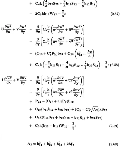
(_b 11 s 11

–b12 S 12 - b22 S22) - (2.58)

O

k f—ouv

= - C8-1u2----+uv-..--_

Ox _{\ Ox Oy}

O

kf

Ouv

_—Ouv

+ - Cs-IflV--+y2---.

Oy

E\ Ox _Oy

+ P12 - (C 1

E+

CPk)b12

+ C2 €(b11 b12 + b22b12 ) + (C 3 - C/X)kS12

+ C4k(bii S i2 + b22 S 12 + b21 s 11 +

b21S22)

+

C5 k(b22 - b 11 )W12 -

2

(2.59)

where

A2 b 1 + b 2 + b 3 + 2b2

(2.60)

The coefficients used here are those recommended by the model

origina-tors and are given in Table 2.3.

[image:47.595.111.509.58.576.2]

C1 C2 c C3 C; c4 c5 c1 c

3.4 4.2 1.8 0.8 1.3 1.25 0.4 1.44 1.8J