Combining MLC and SVM classifiers for learning based decision making : analysis and evaluations

Combining MLC and SVM Classifiers for Learning based Decision Making:

Analysis and Evaluations

Yi Zhang1_{, Jinchang Ren}2, *_{, Jianmin Jiang}3

[email protected], [email protected], [email protected]

1 _{School of Computer Software, Tianjin University, Tianjin, China}

2 _{Centre for excellence in Signal and Image Processing, University of Strathclyde, Glasgow, UK} 3 _{School of Computer Science and Software Engineering, Shenzhen University, Shenzhen, China}

Abstract:

Maximum likelihood classifier (MLC) and support vector machines (SVM) are two commonly used approaches in machine learning. MLC is based on Bayesian theory in estimating parameters of a probabilistic model, whilst SVM is an optimization based non-parametric method in this context. Recently, it is found SVM in some cases is equivalent to MLC in probabilistically modeling of the learning process. In this paper, MLC and SVM are combined in learning and classification, which helps to yield probabilistic output for SVM and facilitate soft decision making. In total four groups of data are used for evaluations, covering sonar, vehicle, breast cancer and DNA sequences. The data samples are characterized in terms of Gaussian/non-Gaussian distributed and balanced/unbalanced sampled, which are then further used for performance assessment in comparing the SVM and the combined SVM-MLC classifier. Interesting results are reported to indicate how the combined classifier may work under various conditions.

Keywords: maximum likelihood classifier (MLC), support vector machines (SVM), machine learning, combined SVM-MLC classifier, knowledge based systems

Corresponding Author:

Dr. Jinchang Ren

Dept. of Electric and Electrical Engineering University of Strathclyde

204 George Street Glasgow, G1 1XW United Kingdom

Tel. +44-141-5482384

1.

Introduction

Maximum likelihood classification (MLC) is one of the most commonly used approach in signal classification and identification, which has been successfully applied in a wide range of engineering applications including classification for digital amplitude-phase modulations [1], remote sensing [2], genes selection for tissue classification [3], nonnative speech recognition [4], chemical analysis in archaeological applications [5] and speaker recognition [6]. On the other hand, support vector machines (SVM) has attracted much increasing attention, which can be found in almost all areas when prediction and classification of signal is required, such as scour prediction on grade-control structure [7], fault diagnosis [8], EEG signal classification [9], and fire detection [10] as well as road sign detection and recognition [11].

Based on the principles of Bayesian statistics, MLC provides a parametric approach in decision making where the model parameters need to be estimated before they are applied for classification. On the contrary, SVM is a non-parametric approach, where the theoretic background is supervised machine learning. Due to the differences of these two classifiers, their performance appears to be much different. Taking the application in remote sensing for example, in Pal and Mather [12] and Huang et al [13], it is found SVM outperforms MLC and several other classifiers. In Waske and Benedijktsson [14], SVM produces better results from SAR images, yet in most cases it generates worse results than MLC from TM images. In Szuster et al [15], SVM only yields slightly better results than MLC for land cover analysis. As a result, detailed assessments as on what conditions SVM outperforms or appears inferior to MLC are worth further investigation.

Furthermore, there becomes a trend to combine the principle of MLC, Bayesian theory, with SVM for improved classification. In Ren et al [16], Bayesian minimum error classification is applied to the predicted outputs of SVM for error-reduced optimal decision-making. Similarly, in Hsu et al [17], Bayesian decision theory is applied in SVM for imbalance measurement and feature optimization for improved performance. In Vega et al [18], Bayesian statistics is combined with SVM for parameter optimization. In Vong et al [19], Bayesian inference is applied to estimate the hyper-parameters used in SVM learning to speed up the training process. In Foody [20], relevance support machine (RVM), a Bayesian extension of SVM is proposed which enables an estimate of the posterior probability of class membership where conventional SVMs fail to do so. Consequently, in-depth analysis of the two classifiers is desirable to discover their pros and cons in machine learning.

In this paper, analysis and evaluations of SVM and MLC is emphasized, using data from various applications. Since the selected data satisfy certain conditions in terms of specific sample distributions, we aim to find out how the performance of the classifiers is connected to the particular data distributions. As a consequence, the work and the results shown in the paper are valuable for us to understand how these classifiers work, which can then provide insightful guidance as how to select and combine them in real applications.

The remaining parts of the paper are organized as follows. Section 2 introduces the principles of the two classifiers. Section 3 describes data and methods that have been used, where experimental results and evaluations are analyzed and discussed in Section 4. Concluding remarks are given in Section 5.

2.

MLC and SVM Revisited

In this section, the principles of the two classifiers, SVM and MLC, are discussed. By comparing their theoretic background and implementation details, the two classifiers are characterized in terms of their performances during the training and testing processes. This in turn has motivated our work in the following sections.

2.1 The Maximum Likelihood Classifier (MLC)

Let

(

,

,...,

,

)

T

,

[

1

,

]

, 2 , 1

,

x

x

i

M

x

i i i N

i





x

be a group of N-dimensional features, derived from M observed samples,

]

,

1

[

C

y

i



denotes the class label associated with

x

i, i.e. in total we have C classes denoted as



c,

c



2

. The basic

also the samples are independent to each other. To this end, the likelihood (probability) for samples within the kth class,



_k, is given as follows.













_

_



₍

₎



₍

₎

2

1

-exp

|

|

)

(2

1

)

|

(

T 1

1/2 c

N/2 c c c

c

p

x

μ

S

x

μ

S

x





(1)

where

μ

_c and

S

_c respectively denote the mean vector and co-variance of all

N

_c samples within



_c, which can be determined using maximum likelihood estimation as



 c N i i c 1 1 -c

N

=

x

μ

(2)

T 1

1

-c

(

)(

)

N

=

N _{i c}

i i c c c

μ

x

μ

x

S









(3)

For a given sample

x

_i, the probability it belongs to class



_c can be denoted as

p

(



_c

|

x

_i

)

. The class

c

that

x

_i

is determined to be within is then decided by



(

|

)



max

arg

)

(

_{c i}

c i

MLC

p

f

x





x

(4)

Based on Bayesian theory, we have

)

(

)

|

(

)

(

)

|

(

i c i c i c

p

p

p

p

x

x

x









(5)

Since

p

(

x

_i

)

is a constant in Eq. (5) when

x

_i is given, Eq. (4) can be re-written as



(

)

(

|

)



max

arg

)

(

_{c i c}

c i

MLC

p

p

f

x





x



(6)

Applying logarithm operation to the right side of Eq. (6), also let

g

_c

(

x

)



ln

p

(

x

|



_c

)



ln

p

(



_c

)

be the discriminating function, Eq. (6) becomes



(

)



max

arg

)

(

_{c i}

c i

MLC

g

f

x



x

(7)

)

(

ln

|

|

ln

2

1

2

ln

2

)

(

)

(

2

1

)

(

T 1

c c c c c c

p

N

g

_x





_x



_u

_S



_x



_u







_S





₍₈₎

Again we can ignore the constant in Eq. (8) and simplify the discriminating function as

c c c c c c c c c

p

g

























x

w

x

W

x

S

u

x

S

u

x

x

T T 1

T

_ln

_|

_|

_ln

₍

₎

2

1

)

(

)

(

2

1

)

(

(9)

where

W

_c





(

2

S

_c

)

1,

w

_c

_

S

_c1

u

_c

and

2

1 T 1

2

1

ln

|

|

ln

(

)

c c

c c c

c

p











_u

_S



_u





_S



.

As can be seen,

g

_c

(

x

)

is now a quadratic function of

x

depending on three parameters, i.e.

u

_c,

S

_c and

p

(



_c

)

. When the class

c

is specified, these parameters are determined, hence the quadratic function only depends on the class

In a particular case when p(



c) is a constant for all

c

, i.e. the prior probability that a sample belongs to one of the

classes is equal, lnp(



c) in Eq. (9) can be ignored hence the discriminating function is re-written as

|

|

ln

)

(

)

(

)

(

T 1

c c

c c c

g

x





x



u

S



x



u



S

₍₁₀₎

where the scalar 1/2 is also ignored as it makes no difference when Eq. (7) is applied for decision-making. However, such simplification cannot be made unless we have clear knowledge about the equal distribution of the samples over the C classes.

Based on Eq. (10), the decision function can be further simplified if the total number of classes is reduced to two, where the two classes are denoted as -1 and 1 and the

sign

function in introduced for simplicity.

|

|

|

|

ln

)

(

)

(

)

(

)

(

)

(

0

)

(

1

0

)

(

1

))

(

(

)

(

1 T 1 T          































S

S

u

x

S

u

x

u

x

S

u

x

x

x

x

x

x

MLC i MLC i MLC i MLC i MLC

g

g

if

g

if

g

sign

f

(11)

Moreover, in a special case when

S

_



S

_



S

, the quadratic decision function in Eq. (11) becomes a linear one as

)

(

2

)

(

)

(

T 1 1 T 1 T 1

         









u

u

S

x

u

S

u

u

S

u

x

MLC

g

(12)

2.2 The Support Vector Machine (SVM)

SVM was originally developed for the classification of two-class problem. In Cortes and Vapnik [22], the principles of SVM are comprehensively discussed. Let the two classes denoted as 1 and -1, similar to the decision function for MLC in Eq. (11), the decision function for linear SVM is given by

b

g

g

if

g

if

f

y

i i SVM i SVM i SVM i SVM i























x

w

x

x

x

x

T

)

(

1

)

(

1

1

)

(

1

)

(

(13)

where

y

_i denotes the labeled value for the input sample

x

_i;

w

and

b

are parameters to be determined in the training process.

Note that the decision function in Eq. (13) is actually equivalent to the one in Eq. (11) if we adjust the scalar for

b

,

yet Eq. (13) is more feasible as it has increased the decision margin between the two classes from near zero to

2

|

_w

|

1_{. By}

multiplying

y

_i to both sides of the discriminating function

g

, this can be further simplified as

y

_i

g

_SVM

(

x

_i

)



1

, i.e.

1

)

(

T

_

_b

_

y

_i

w

x

_i (14)

Hence, the optimal hyperplane to separate the training data with a maximal margin is defined by

0

T

_

_

o o

x

b

w

(15)

where

w

_oand

b

_o are the determined parameters, and the maximal distance becomes

2

|

|

1

o

w

.

To determine this optimal hyperplane, we need maximize

2

|

w

|

1 , or equivalently to minimize

2

1

|

w

|

2, subject

to



x

_i,

_y

(

T

_

_b

)

_

1

i



(

)

1



.

.

0

2

1

)

,

,

(

T 1 2















 i i i

L i

i

i

y

b

s

t

b



w



w

x



w

(16)

Eventually, the parameters

w

_o and

b

_o are decided as

0

,

T 1











 i o i i

L i

i i i

o



y

x

b

y

w

x

where



w

(17)

For any non-zero



_i , the corresponding

x

_i is denoted as one support vector which naturally satisfies

1

)

(

T

_

_b

_

y

_i

w

x

_i . Therefore,

w

_o is actually the linear combination of all support vectors. Also we have





_i

y

_i



0

. Eventually if we combine Eq. (17) with Eq. (13), the discrimination function for any test sample

x

becomes

b

y

g

L i i i i

SVM







1 T

)

(

x



x

x

(18)

which solely relies on the inner product of the support vector and the test sample.

For nonlinear problems which are not linearly separable, the discrimination function is extended as

b

K

y

b

y

g

L i i i i L i i i i

SVM















1 1

T

₍

₎

₍

_,

₎

)

(

)

(

x





x



x



x

x

(19)

where



aims to map the input samples to another space thus makes them linearly separable.

Another important step is to introduce the kernel trick to calculate the inner product of mapped samples, i.e.







(

x

_i

),



(

x

)

, which avoids the difficulty in determining the mapping function



and also the cost for calculation of the mapped samples and their inter-product. Several typical kernels including linear, polynomial and radial basis function (RBF) are summarized below.





























RBF

polynomial

p

linear

K

j i p j i j i j i

)

2

exp(

0

,

)

1

(

)

,

(

2 2 T T



x

x

x

x

x

x

x

x

(20)

where optimal values for the associated parameters

p

and



are determined automatically during the training process. Though SVM is initially developed for two-class problems, it has been extended to deal with multi-class classification based on either combination of decision results from multiple two-class classification or optimization on multi-class based learning. Some useful further readings can be found in [23], [24] and [25].

2.3 Analysis and Comparisons

MLC and SVM are two useful tools for classification problems, where both of them rely on supervised learning in determining the model and parameters. However, they are different in several ways as summarized below.

Firstly, MLC is a parametric approach which has a basic assumption that the data satisfy Gaussian distribution. On the other contrary, SVM is a non-parametric approach and it has no requirement on the prior distribution of the data, yet various kernels can be empirically selected to deal with different problems.

are applied for testing and prediction. However, SVM relies on supervised machine learning, in an iterative way, to

determine a large amount of parameters including

w

_o,

b

_o, all non-zero



_i and their corresponding support vectors. Thirdly, MLC can be straightforward applied to two-class and multi-class problems, yet additional extension is needed for SVM to deal with multi-class problem as it is initially developed for two-class classification.

Finally, a posterior class probabilistic output for the predicted results can be intuitively generated from MLC, which is a valuable indicator for classification to show how likely a sample belongs to a given class. For SVM, however, this is not an easy task though some extensions have been introduced to provide such an output based on the predicted value from

SVM. In Platt [26], a posterior class probability

p

_i is estimated by a sigmoid function below.

)

)

(

exp(

1

1

)

|

1

(

B

Ag

y

P

p

i SVM i

i





x



_

_x

_

(21)

The parameters

A

and

B

are determined by solving a regularized maximum likelihood problem as follows.

















_

_

_

_





 L

i i i i i

B A

p

t

p

t

B

A

1 ) , (

)

1

log(

)

1

(

)

log(

min

arg

*)

*,

(

(22)























)

1

2

/(

1

1

)

2

/(

)

1

(

1 1 1 i i

i

_N

_if

_y

y

if

N

N

t

(23)

where

N

₁ and

N

_1 denote the number of support vectors labeled in class 1 and -1, respectively.

In addition, in Lin et al [27] Platt’s approach is further improved to avoid any numerical difficulty, i.e. overflow or

underflow, in determining

p

_i in cases

E

_i



Ag

_SVM

(

x

_i

)



B

is either too large or too small.

















_  

otherwise

e

e

E

if

e

p

i i i E E i E i ₁ 1

)

1

(

0

)

1

(

(24)

Although there are significant differences between SVM and MLC, the probabilistic model above has uncovered the connection between these two classifiers. Actually, in Franc et al [21] MLC and SVM are found to be equivalent to each other in linear cases, and this can also be convinced by the similar decision functions in Eq. (11) and Eq. (13).

3.

Data and Methods

In this paper, analysis and evaluations of SVM and MLC is emphasized, using data from various applications. Since the selected data satisfy certain conditions in terms of specific sample distributions, we aim to find out how the performance of the classifiers is connected to the particular data distributions. As a consequence, the work and the results shown in the paper are valuable for us to understand how these classifiers work, which can then provide insightful guidance as how to select and combine them in real applications.

3.1 The datasets

in another class. On the other hand, the last two datasets are quite balanced. Regarding feature distributions, samplesNew and svmguide3 are apparently non-Gaussian distributed, yet the other two, sonar and splice, show approximately Gaussian characteristics when the variables are separately observed. This is also validated by the determined Pearson’s moment

coefficient of skewness below [30], where



_i and



_i are the mean and standard deviation for the

i

th dimension of the dataset, and

E

(.)

refers to mathematical expectation. When the skewness coefficients are determined for each data dimension, the maximum, the minimum and the average skewness coefficients are obtained and shown in Table 1 for comparisons.

3 3

)

(

i i i i

x

E

S









(25)

Table1. Four datasets used in our experiments

Dataset Features Balance Status

Distribution of feature value

Number of samples

(Class 0 /Class 1)

Skewness coefficients

max min mean samplesNew 39 Unbalanced Not-Gaussian Approx. 748 (115/633) 7.577 -3.063 2.343 svmguide3 21 Unbalanced Not-Gaussian Approx. 1284 (947/337) 10.074 -4.653 2.181 sonar 31 Balanced Approx. Gaussian 209 (97/102) 1.123 -1.019 0.214 splice 60 Balanced Approx. Gaussian 1269 (653/616) 0.672 -0.490 -0.016

3.2 The approach

In our approach, a combined classifier using SVM and MLC is applied, which contains the following three stages. In Stage 1, SVM is used for initial training and classification. For the correctly classified results in SVM, these are employed in Stage 2, where MLC is applied for probability based modeling. The probability-based models are then utilized in Stage 3 for improved decision making and better classification. Details of these three stages are discussed as follows.

Stage 1: SVM for initial training and classification

The open source library libSVM [28] is used for initial training and classification of the aforementioned four datasets, and both the linear and the Gaussian radial basis (RBF) kernels are tested. For each group of datasets, all the data are normalized to [-1, 1] before SVM is applied. Through 5-fold cross validation, the best group of parameters, including the cost and the gamma value, are optimally determined. Eventually, the optimal parameters are used for classification of our datasets.

In our experiments, the training ratios are set at three different levels, i.e. 80%, 65% and 50%. Basically, there is no overlap between training data and testing data. At a given training ratio, the training data is randomly selected and repeated five times, which leads to 5 groups of test results generated. Finally, the average performance over these five experiments is used for comparisons.

Stage 2: Using MLC for probability-based modeling

For those correctly classified samples, which lie in two classes, i.e. class 0 and class 1, they are taken to decide two probability-based models, in a way as discussed in MLC. In other words, for samples correctly classified in class 0, they are used to determine the mean vector and the corresponding co-variance matrix within class 0. On the other hand, samples which are correctly classified in class 1 are used to determine the mean vector and the corresponding co-variance matrix within class 1. Note that not all samples in class 0 or class 1 are used in calculating the related MLC models, as those which cannot be correctly classified by SVM are treated as outliers and ignored in MLC modeling for robustness.

After MLC modeling, for each sample

x

, the associated likelihoods that it belongs to the two classes are re-calculated













otherwise

p

p

if

f

_MLC

0

)

(

)

(

1

)

(

_x

1

x

0

x



(26)

where



is a threshold to be optimally determined to generate the best classified results. Please note that the likelihoods (or probability values) here can also be taken as a probabilistic output of the SVM.

Stage 3: Improved classification

With the estimated MLC models and the optimal threshold



, all samples are then re-checked for improved

classification, using (25) and the determined likelihoods p0(x) and p1(x), accordingly. Interesting results on these four

datasets are given and analyzed in detail in the next Section.

4.

Results and Evaluations

For the four datasets discussed in Section 3, the experimental results are reported and analyzed in this section. Firstly, we discuss results from a combined classifier of MLC and a linear SVM. Then, results from MLC and RBF based SVM are compared. In addition, how different re-balancing strategies affect the performance of unbalanced datasets is also discussed.

4.1 Results from a linear SVM and the MLC

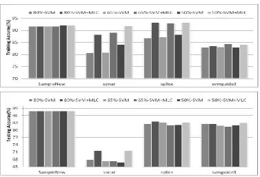
In this group of experiments, a combined classifier using a linear SVM and the MLC is employed, and the relevant results are presented in Fig. 1. In Fig. 1, we plot the classification rate as the prediction accuracy with the change of training ratio, i.e. the percentage of data used for training. Three training ratios, 80%, 65% and 50% are used. Please note that due to degradation of the co-variance matrix, the MLC cannot be used to improve the results for the SampleNew dataset. Consequently, the results from the SVM are taken as the output of the combined classifier. For the other three datasets, the results are summarized and compared as follows.

Firstly, for the three datasets, Sonar, Splice and svmguide3, apparently we can see that the combined solution yield significantly improved results in training, especially for the first two datasets. This demonstrates that the combined classifier can indeed achieve more accurate modeling of the datasets. In addition, possibly due to over-fitting, it shows that a larger training ratio does not necessarily improve the training performance.

[image:8.595.110.488.513.770.2]

However, the testing results are some different. For the Sonar dataset, which is balanced and appears near Gaussian distributed, the combined classifier yields much improved results in testing, especially when the training ratios are 80% and 50%. Such results are not surprising as the MLC is ideal to model Gaussian-alike distributed datasets. For the Splice dataset, which is balanced and also nearly Gaussian distributed, slightly improved testing results are also produced by the combined classifier at training ratios at 80% and 50%, but the testing results at the training ratio of 65% becomes slightly worse than those from the SVM. For the more challenging svmguide3 dataset, which is unbalanced and non-Gaussian distributed, although the combined classifier yields improved testing results at the training ratio of 50%, the results at the other two training ratios, perhaps due to over-fitting, seem inferior to the results from the SVM. Actually, in nature the MLC has difficulty in modeling non-Gaussian distributed datasets, and this explains where the combined classifier makes less contribution to these datasets.

4.2 Results from a RBF-kernelled SVM and the MLC

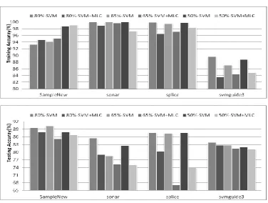
In this group of experiments, the RBF kernel is used for the SVM in the combined classifier as it is popularly used in various classification problems [16, 23]. For the four datasets we used, again the training results and the testing results under three different training ratios are summarized and given in Fig. 2 for comparisons.

First of all, RBF-kernelled SVM (R-SVM) produces much improved results than those using linear SVM, especially for the training results. In fact, the combined classifier generates better results than the SVM only in the SampleNew dataset, slightly worse results in sonar and splice datasets, and much degraded results in the svmguide3 dataset.

Regarding testing results, although the combined classifier generates comparable or slightly worse results in the SampleNew dataset and the svmguide3 dataset, R-SVM yields better results in splice dataset and sonar dataset. The reason behind is that results from the non-linear kernel in R-SVM cannot be directly refined using MLC. Also, occasionally the results from the combined classifier seem more sensitive to the training ratio, especially for the splice dataset, which is perhaps due to the threshold to be determined depends more or less on the training data used.

Figure 2. Comparing training (top) and testing results (bottom) using RBF kernelled SVM and the combined classifier for the four datasets under three different training ratios.

4.3 Testing on Re-balanced Data

[image:9.595.110.487.443.727.2]

unbalanced data may affect the classification performance is analyzed. For the unbalanced dataset, samples from one class may be over-represented than those in another class. As a result, we can either over-sampling the data of minority or sub -sampling the data of majority to balance the number of samples represented in the training set for better modeling of the data. On the other hand, the test samples remain to be unbalanced as it is assumed we have no label information for the test samples.

For over-sampling, data samples which are in minority class are randomly duplicated and inserted into the dataset. The replication of data items continues until the entire training set becomes balanced. Different from over-sampling, sub-sampling randomly discards samples from the majority class until the training set achieves balanced. Since the performance may be affected by samples duplicated or discarded, this process is repeated for over 10 times and the average performance is then recorded for comparisons.

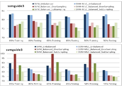
Using three different training ratios at 80%, 65% and 50%, results of balanced learning for the svmguide3 dataset are summarized in Fig. 3. Under a given training ratio, both training results and testing results are presented in groups, where each group contains results from 6 different experimental scenarios. In addition, the results from liner SVM and RBF-kernelled SVM are shown for comparisons as well.

When linear SVM is used, as shown in the first row of Fig. 3, surprisingly, the results from unbalanced data are much better than those from balanced data. Also in majority cases, the combined classifier outperforms the SVM classifier in both training and testing, even with balanced learning introduced. The testing results from SVM for balanced learning via over-sampling seem better than those from sub-sampling, yet it seems that the combined classifier produces better results from sub-sampling based balanced learning.

[image:10.595.102.494.424.701.2]

For RBF-kernelled SVM, apparently, the training results from SVM via over-sampling are among the best, though the testing results are inferior to those from un-balanced training. This indicates that the training process has been over-fitting in this context. In fact, testing results from the combined classifier are slightly worse than those from the SVM classifier, i.e. some degradation. Again, this is caused by the inconsistency of the non-linear SVM and the linear nature of the MLC.

Fig. 3: Results of balanced learning for the svmguide3 dataset, using linear SVM (top) and R-SVM (bottom).

5.

Conclusions

work effectively needs to be explored. In this paper, comprehensive results are demonstrated to answer the question above, using four different datasets. First of all, it is found that the combined classifier works under certain constraints, such as a linear SVM, balanced dataset and near Gaussian-distributed data. When a RBF-kernelled SVM is used, the combined classifier may produce degraded results due to the inconsistency between the non-linear kernel in SVM and linear nature of MLC. In addition, for a challenging dataset, balanced learning may improve the results of training but not necessaries the testing results. The reason behind is that the combined SVM-MLC classifier works on three assumptions, i.e. Gaussian distributed, inter-class separable, and model consistency between training data and testing data. Although the third assumption is true in most cases, the precondition of separable Gaussian distributed data is rather a strict constraint for data and rarely be satisfied. As a result, this introduces a fundamental difficulty in combining these two classifiers. However, under certain circumstances, the combined classifier indeed can significantly improve the classification performance. It is worth noting that when more groups is introduced in modelling a given dataset the efficacy can be severely degraded due to the inconsistency of statistical distribution between groups. Future work will focus on combining other classifiers such as neural network for applications in medical imaging [31-33] and recognition and classification tasks [34-35].

6.

References

[1]Wei, W., Mendel, J.M., Maximum-likelihood classification for digital amplitude-phase modulations. IEEE Trans. Commun. 48 (2), 189–193, 2000. [2] Liu, K., Shi, W., Zhang,, H., A fuzzy topology-based maximum likelihood classification, ISPRS Journal of Photogrammetry and Remote Sensing, 66(1): 103-114, 2011

[3] Huang, H.-L., Lee, C.-C., Ho, S.-Y., Selecting a minimal number of relevant genes from microarray data to design accurate tissue classifiers, Biosystems, 90(1): 78-86, 2007

[4] He, X., Zhao, Y., Prior knowledge guided maximum expected likelihood based model selection and adaptation for nonnative speech recognition, Computer Speech and Language, 21(2): 247-265, 2007

[5] Hall, M., Minyaev, S., Chemical analyses of Xiong-nu pottery: a preliminary study of change and trade on the inner Asia steppes, Journal of Archaeological Science, 29(2): 135-144, 2002

[6] Hong, Q.Y., Kwong, S., A genetic classification method for speaker recognition, Engineering Applications of Artificial Intelligence, 18(1): 13-19, 2005 [7] Goel, A., Pal, M., Application of support vector machines in scour prediction on grade-control structure, Engineering Applications of Artificial Intelligence, 22(2): 216-223, 2009

[8] Yelamos, I., Escudero, G., Graells, M., Puigjaner, L., Performance assessment of a novel fault diagnosis system based on support vector machines, Computers and Chemical Engineering, 33(1): 244-255, 2009

[9] Subasi, A., Gursoy, M.I., EEG signal classification using PCA, ICA, LDA and support vector machines, Expert Systems with Applications, 37(12): 8659-8666, 2010

[10] Ko, B.C., Cheong, K.-H., Nam, J.-Y., Fire detection based on vision sensor and support vector machines, Fire Safety Journal, 44(3): 322-329, 2009 [11] Maldonado-Bascon, S., Road-sign detection and recognition based on support vector machines, IEEE Trans. Intelligent Transportation Systems, 8(2): 264-278, 2007

[12] Pal, M., Mather, P.M., Assessment of the effectiveness of support vector machines for hyperspectral data, Future Generation Computer Systems, 20(7): 1215-1225, 2004.

[13] Huang, C., Davis, L.S., Townshend, J.R.G., An assessment of support vector machines for land cover classification, Int. J. Remote Sensing, 23(4): 725-749, 2002.

[14] Waske, B., Benedijktsson, J.A., Fusion of support vector machines for classification of multisensor data, IEEE Trans. Geoscience and Remote Sensing, 45(12): 3858-3866, 2007.

[15] Szuster, B.W., Chen, Q., Borger, M., A comparison of classification techniques to support land cover and land use analysis in tropical coastal zones, Applied Geography, 31: 525-532, 2011

[16] Ren, J., ANN vs. SVM: which one performs better in classification of MCCs in mammogram imaging, Knowledge Based System, 26(2): 144-153, 2012 [17] Vong, C.-M., Wong, P.-K., Li, Y.-P., Prediction of automotive engine power and torque using least squares support vector machines and Bayesian inference, Engineering Applications of Artificial Intelligence, 19(3): 277-287, 2006

[19] Hsu, C.-C., Wang, K.-S., Chang, S.-H., Bayesian decision theory for support vector machines: imbalance measurement and feature optimization, Expert Systems with Applications, 38(5): 4698-4704, 2011

[20] Foody, G.M., RVM-based multi-class classification of remotely sensed data, Int. Journal. Remote Sensing, 29(6): 1817-1823, 2008. [21] Franc, V., Zien, A., Scholkopf, B., Support vector machines as probabilistic models, in Proc. 28th _{Int. Conf. Machine Learning, 2011}

[22] Cortes, C., Vapnik, V., Support-vector networks, Machine Learning, 20: 273-297, 1995

[23] Hsu, C.-W., Lin, C.-J., A Comparison of Methods for Multiclass Support Vector Machines, IEEE Transactions on Neural Networks, 13(2): 415-425, 2002 [24] Lee, Y., Lin, Y., Wahba, G., Multicategory Support Vector Machines, Theory, and Application to the Classification of Microarray Data and Satellite Radiance Data, J. Amer. Statist. Assoc. 99(465): 67-81, 2004.

[25] Crammer, K., Singer, Y., On the Algorithmic Implementation of Multiclass Kernel-based Vector Machines, Journal of Machine Learning Research 2: 265–292, 2001

[26] Platt, J., Probabilistic Outputs for Support Vector Machines and Comparisons to Regularized Likelihood Methods, In: A. Smola, P. Bartlett, B. Scholkopf, and D. Schuurmans (eds.): Advances in Large Margin Classifiers. Cambridge, MA., 2000

[27] Lin, H.-T., Lin, C. J., Weng, R. C., A note on Platt’s probabilistic outputs for support vector machines, Journal of Machine Learning, 68(3): 267-276, 2007.

[28] Chang, C.-C., Lin, C.-J., LIBSVM: a library for support vector machines. ACM Transactions on Intelligent Systems and Technology, 2:27:1--27:27, 2011. Software available at http://www.csie.ntu.edu.tw/~cjlin/libsvm

[29] Frank, A., Asuncion, A. UCI Machine Learning Repository, http://archive.ics.uci.edu/ml/datasets.html

[30] Doane, D. P. and Seward, L. E., Measuring skewness: a forgotten statistics?, Journal of Statistics Education, 19(2):1-18, 2011

[31] Jiang, J., Trundle, P., Ren, J., Medical image analysis with artificial neural networks, Computerized medical Imaging and Graphics, 34(8): 617-631, 2010 [32] Ren, J., ANN vs. SVM: which one performs better in classification of MCCs in mammogram imaging, Knowledge-Based Systems, 26:144-153, 2012 [33] Ren, J., Wang, D., Jiang, J., effective recognition of MCCs in mammograms using an improved neural classifier, Engineering Applications of Artificial Intelligence, 24(4): 638-645, 2011

[34] Zhao, C., Li, X., Ren, J., Marshall, S., Improved sparse representation using adaptive spatial support for effective target detection in hyperspectral imagery, Int. J. Remote Sensing, 34(24): 8669-8684, 2013