OPTIMIZED SCHWARZ METHODS FOR MAXWELL’S EQUATIONS
∗V. DOLEAN†, M.J. GANDER‡,AND L. GERARDO-GIORDA§
Abstract. Over the last two decades, classical Schwarz methods have been extended to systems of hyperbolic partial differential equations, using characteristic transmission conditions, and it has been observed that the classical Schwarz method can be convergent even without overlap in certain cases. This is in strong contrast to the behavior of classical Schwarz methods applied to elliptic problems, for which overlap is essential for convergence. More recently, optimized Schwarz methods have been developed for elliptic partial differential equations. These methods use more effective transmission conditions between subdomains than the classical Dirichlet conditions, and optimized Schwarz methods can be used both with and without overlap for elliptic problems. We show here why the classical Schwarz method applied to both the time harmonic and time discretized Maxwell’s equations converges without overlap: the method has the same convergence factor as a simple opti-mized Schwarz method for a scalar elliptic equation. Based on this insight, we develop an entire new hierarchy of optimized overlapping and nonoverlapping Schwarz methods for Maxwell’s equations with greatly enhanced performance compared to the classical Schwarz method. We also derive for each algorithm asymptotic formulas for the optimized transmission conditions, which can easily be used in implementations of the algorithms for problems with variable coefficients. We illustrate our findings with numerical experiments.
Key words. Schwarz algorithms, optimized transmission conditions, Maxwell’s equations
AMS subject classifications.65M55, 65F10, 65N22
DOI.10.1137/080728536
1. Introduction.
Schwarz algorithms experienced a second youth over the last
decades when distributed computers became more and more powerful and available.
Fundamental convergence results for the classical Schwarz methods were derived for
many partial differential equations and can now be found in several authoritative
re-views [3, 41, 42] and books [34, 33, 39]. The Schwarz methods were also extended
to systems of partial differential equations, such as the time harmonic Maxwell’s
equations [12, 8], the time discretized Maxwell’s equations [38], or to linear elasticity
[18, 19], but much less is known about the behavior of the Schwarz methods applied to
hyperbolic systems of equations. This is true, in particular, for the Euler equations,
to which the Schwarz algorithm was first applied in [31, 32], where classical
(char-acteristic) transmission conditions are used at the interfaces, or with more general
transmission conditions in [7]. The analysis of such algorithms applied to systems
proved to be very different from the scalar case; see [14, 15].
Over the last decade, a new class of overlapping Schwarz methods was
devel-oped for scalar partial differential equations, namely, the optimized Schwarz
meth-ods. These methods are based on a classical overlapping domain decomposition, but
they use more effective transmission conditions than the classical Dirichlet conditions
at the interfaces between subdomains. New transmission conditions were originally
proposed for three different reasons: first, to obtain Schwarz algorithms that are
con-vergent without overlap; see [28] for Robin conditions. The second motivation for
∗Received by the editors June 25, 2008; accepted for publication (in revised form) December 5,
2008; published electronically May 7, 2009.
http://www.siam.org/journals/sisc/31-3/72853.html
†Laboratoire J.-A. Dieudonn´e, Univ. de Nice Sophia-Antipolis, Nice, France ([email protected]). ‡Section de Math´ematiques, Universit´e de Gen`eve, CP 64, 1211 Gen`eve, Switzerland (martin.
§Department of Mathematics, University of Trento, Trento, Italy ([email protected]).
2193
changing the transmission conditions was to obtain a convergent Schwarz method
for the Helmholtz equation, where the classical overlapping Schwarz algorithm is
not convergent. As a remedy, approximate radiation conditions were introduced in
[10, 12]. The third motivation was that the convergence rate of the classical Schwarz
method is rather slow and too strongly dependent on the size of the overlap. In
a short note on nonlinear problems [26], Hagstrom, Tewarson, and Jazcilevich
in-troduced Robin transmission conditions between subdomains and suggested
nonlo-cal operators for the best performance. In [4], these optimal, nonlononlo-cal transmission
conditions were developed for advection-diffusion problems, with local
approxima-tions for small viscosity, and low order frequency approximaapproxima-tions were proposed in
[29, 9]. In [35], one can find low-frequency approximations of absorbing boundary
conditions for the Euler equations. Independently, at the algebraic level,
general-ized coupling conditions were introduced in [37, 36] for discrete overlapping Schwarz
methods. Optimized transmission conditions for the best performance of the Schwarz
algorithm in a given class of local transmission conditions were first introduced for
advection-diffusion problems in [27], for the Helmholtz equation in [6, 24], and for
Laplace’s equation in [17]. For complete results and attainable performance for a
symmetric, positive definite problem, see [20], and for time dependent problems, see
[23, 21]. The purpose of this paper is to design and analyze a family of optimized
overlapping and nonoverlapping Schwarz methods for Maxwell’s equations, both for
the case of time discretized and time harmonic problems, and to provide explicit
formulas for the optimized parameters in the transmission conditions of each
algo-rithm in the family. These formulas can then easily be used in implementations for
Maxwell’s equations with variable coefficients. As we will see, one member of this
family reduces in the case of no overlap and constant coefficients to an algorithm in
a curl-curl formulation of Maxwell’s equations, proposed in [1] based on [5], which
already greatly enhanced the performance compared to the classical approaches in
[12, 8].
This paper is organized as follows: in section 2, we present Maxwell’s equations
and a reformulation thereof with characteristic variables used in our analysis. In
section 3, we treat the case of time harmonic solutions. We show that the classical
Schwarz method for Maxwell’s equations, which uses characteristic Dirichlet
transmis-sion conditions between subdomains, is convergent even without overlap. Exploiting
a relation with an optimized Schwarz method applied to a Helmholtz equation allows
us to develop an entirely new hierarchy of optimized Schwarz methods for Maxwell’s
equations with greatly enhanced performance, both with and without overlap. A
sim-ilar relation has been used in [13] for the Cauchy–Riemann equations. In section 4,
we present and analyze the corresponding hierarchy of optimized Schwarz methods
for time discretizations of Maxwell’s equations. We then show in section 5 numerical
experiments in two and three spatial dimensions, both for the time harmonic and
time discretized cases, which illustrate the performance of the new optimized Schwarz
methods for Maxwell’s equations. We also include as an application the cooking of
a chicken in a microwave oven, a problem with variable coefficients. In section 6, we
summarize our findings and conclude with an outlook on future research directions.
2. Maxwell’s equations.
The hyperbolic system of Maxwell’s equations
de-scribes the propagation of electromagnetic waves. It is given by
(2.1)
−
ε
∂
E
∂t
+ curl
H
−
σ
E
=
J
,
μ
∂
H
∂t
+ curl
E
= 0
,
where
E
= (
E
1,
E
2,
E
3)
Tand
H
= (
H
1,
H
2,
H
3)
Tdenote the electric and magnetic
fields, respectively,
ε
is the
electric permittivity
,
μ
is the
magnetic permeability
,
σ
is the
electric conductivity
, and
J
is the applied current density. We assume the
applied current density to be divergence free, that is, div
J
= 0. Denoting the vector
of physical unknowns by
(2.2)
u
= (
E
1,
E
2,
E
3,
H
1,
H
2,
H
3)
T,
Maxwell’s equations (2.1) can be rewritten in the form
(2.3)
(
G
+
G
0∂t
)
u
+
Gx∂x
u
+
Gy∂y
u
+
Gz∂z
u
= (
J
;
0
)
,
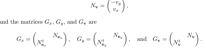
where the coefficient matrices are
G
=
σI
30
3, G
0=
εI
3μI
3, Gl
=
Nl
−
Nl
,
l
=
x, y, z,
where 0
3(resp.,
I
3) represent the 3
×
3 zero (resp., identity) matrix, and the matrices
Nl
,
l
=
x, y, z
, are given by
Nx
=
⎡
⎣
0
0
0
0
0
1
0
−
1
0
⎤
⎦
,
Ny
=
⎡
⎣
0
0
0
0
−
0
1
1
0
0
⎤
⎦
,
Nz
=
⎡
⎣
−
0
1
1
0
0
0
0
0
0
⎤
⎦
.
For any unit vector
n
= (
n
1, n
2, n
3),
n
= 1, we can define the characteristic matrix
of system (2.3) by
C
(
n
) =
G
−01n
1Nx
−
Nx
+
n
2Ny
−
Ny
+
n
3Nz
−
Nz
,
whose eigenvalues are the characteristic speed of propagation along the direction
n
.
A direct calculation shows that the matrix
C
(
n
) has real eigenvalues
λ
1,2=
−
c,
λ
3,4= 0
,
λ
5,6=
c,
with
c
=
√1εμbeing the wave speed. This implies that Maxwell’s equations are
hyper-bolic, since the eigenvalues are real, but not strictly hyperhyper-bolic, since the eigenvalues
are not distinct; see [2]. For the special case of the normal vector
n
= (1
,
0
,
0), which
we will use extensively later, we obtain
C
(
n
) =
1ε
Nx
−
1μ
Nx
,
whose matrix of eigenvectors is given by
L
=
⎡
⎢
⎢
⎢
⎢
⎢
⎢
⎣
0
0
0
1
0
0
−
Z
0
0
0
Z
0
0
Z
0
0
0
−
Z
0
0
1
0
0
0
0
1
0
0
0
1
1
0
0
0
1
0
⎤
⎥
⎥
⎥
⎥
⎥
⎥
⎦
,
where
Z
=
μεdenotes the impedance. This leads to the characteristic variables
w
= (
w
1, w
2, w
3, w
4, w
5, w
6)
T=
L
−1u
associated with the direction
n
, where
(2.4)
w
1=
−
21(
Z1E
2− H
3)
,
w
2=
21(
Z1E
3+
H
2)
,
w
3=
H
1,
w
4=
E
1,
w
5=
12(
Z1E
2+
H
3)
,
w
6=
−
21(
Z1E
3− H
2)
.
In the following, we will denote by
w
+,
w
0, and
w
−the characteristic variables
associated with the negative, zero, and positive eigenvalues, respectively, that is,
(2.5)
w
−= (
w
1, w
2)
T,
w
0= (
w
3, w
4)
T,
w
+= (
w
5, w
6)
T.
Imposing classical or characteristic boundary conditions on a boundary with unit
outward normal vector
n
= (1
,
0
,
0) means to impose Dirichlet conditions on the
incoming characteristic variables
w
−. For a general normal vector
n
, this is equivalent
to imposing the impedance condition (see [2])
(2.6)
B
n(
E
,
H
) :=
n
×
E
Z
+
n
×
(
H
×
n
) =
s
.
3. Time harmonic solutions.
Time harmonic solutions of Maxwell’s equations
are complex-valued static vector fields
E
and
H
such that the dynamic fields
E
(
x
, t
) =
R
e
(
E
(
x
) exp(
iωt
))
,
H
(
x
, t
) =
R
e
(
H
(
x
) exp(
iωt
))
satisfy Maxwell’s equations (2.1). The positive real parameter
ω
is called the
pulsation
of the harmonic wave. The harmonic solutions
E
and
H
satisfy the time harmonic
Maxwell’s equations
(3.1)
−
iωε
E
+ curl
H
−
σ
E
=
J
,
iωμ
H
+ curl
E
=
0
.
3.1. Classical and optimized Schwarz algorithm.
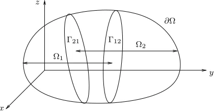
We consider now the
problem (3.1) in a bounded domain Ω, with either Dirichlet conditions on the tangent
electric field or impedance conditions, on
∂
Ω, in order to obtain a well-posed problem;
see [30]. In order to explain the classical Schwarz algorithm for Maxwell’s equation,
we decompose the domain into two overlapping subdomains Ω
1and Ω
2as illustrated
in Figure 3.1. The generalization of the algorithm formulation to the case of many
subdomains does not present any difficulties. The classical Schwarz algorithm then
x
y z
Ω1
Ω2
Γ12
Γ21
[image:4.612.152.363.557.667.2]∂Ω
Fig. 3.1.Overlapping domain decomposition.
solves for
n
= 1
,
2
, . . .
the subdomain problems
(3.2)
−
iωε
E
1,n+ curl
H
1,n−
σ
E
1,n=
J
in Ω
1,
iωμ
H
1,n+ curl
E
1,n=
0
in Ω
1,
B
n1E
1,n,
H
1,n=
B
n1
E
2,n−1,
H
2,n−1on Γ
12
,
−
iωε
E
2,n+ curl
H
2,n−
σ
E
2,n=
J
in Ω
2,
iωμ
H
2,n+ curl
E
2,n=
0
in Ω
2,
B
n2E
2,n,
H
2,n=
B
n2
E
1,n−1,
H
1,n−1on Γ
21
,
where Γ
12=
∂
Ω
1∩
Ω
2, Γ
21=
∂
Ω
2∩
Ω
1, and
B
nj,
j
= 1
,
2, denotes the impedance
boundary conditions defined in (2.6). On the physical part of the boundary, the given
boundary conditions are imposed. While the choice of transmission conditions
B
njis natural in the view of the hyperbolic nature of the problem, we will see in our
analysis that there are better choices for the performance of the algorithm, based on
the notion of absorbing boundary conditions. This leads to the so-called optimized
Schwarz methods
(3.3)
−
iωε
E
1,n+ curl
H
1,n−
σ
E
1,n=
J
in Ω
1,
iωμ
H
1,n+ curl
E
1,n=
0
in Ω
1,
(
B
n1+
S
1B
n2)
E
1,n,
H
1,n= (
B
n1+
S
1B
n2)
E
2,n−1,
H
2,n−1on Γ
12,
−
iωε
E
2,n+ curl
H
2,n−
σ
E
2,n=
J
in Ω
2,
iωμ
H
2,n+ curl
E
2,n=
0
in Ω
2,
B
n2+
S
2B
n1)(
E
2,n
,
H
2,n=
B
n2
+
S
2B
n1)(
E
1,n−1
,
H
1,n−1on Γ
21
,
where
S
j,
j
= 1
,
2, are tangential, possibly pseudodifferential operators we will study
in what follows in order to obtain various optimized Schwarz methods.
3.2. Convergence analysis for the classical Schwarz algorithm.
We now
study properties of the classical Schwarz algorithm (3.2). We use Fourier analysis
and, thus, assume that the coefficients are constant, and the domain on which the
original problem is posed is Ω =
R
3, in which case we need for Maxwell’s equations
the Silver–M¨
uller radiation condition
(3.4)
lim
r→∞
r
(
H
×
n
−
E
) = 0
,
where
r
=
|
x
|
and
n
=
x
/
|
x
|
, in order to obtain well-posed problems; see [30]. The
two subdomains are now half-spaces
(3.5)
Ω
1= (0
,
∞
)
×
R
2,
Ω
2= (
−∞
, L
)
×
R
2,
the interfaces are Γ
12=
{
L
} ×
R
2and Γ
21=
{
0
} ×
R
2, and the overlap is
L
≥
0. We
denote by
ky
and
kz
the Fourier variables corresponding to a transform with respect
to
y
and
z
, respectively, and
|
k
|
2=
k
y2+
k
2z.
Theorem 3.1.
For any given initial guess
(
E
1,0;
H
1,0)
∈
(
L
2(Ω
1))
6,
(
E
2,0;
H
2,0)
∈
(
L
2(Ω
2))
6, the classical Schwarz algorithm
(3.2)
with overlap
L
≥
0
, including the
nonoverlapping case, is for
σ >
0
convergent in
(
L
2(Ω
1))
6×
(
L
2(Ω
2))
6, and the
con-vergence factor for each Fourier mode
k
is
(3.6)
ρcla
(
k
,
ω, σ, Z, L
˜
) =
|
k
|
2−
ω
˜
2+
i
ωσZ
˜
−
i
ω
˜
|
k
|
2−
ω
˜
2+
i
ωσZ
˜
+
i
ω
˜
e
−√
|k|2−ω˜2+iωσZL˜
,
where
ω
˜
=
ω
√
εμ
and
Z
=
μεis the impedance as before.
Proof
. Because of linearity, it suffices to analyze the convergence to the zero
solution when the right-hand side vanishes. Performing a Fourier transform of system
(3.1) in the
y
and
z
directions, the first and the fourth equations provide an algebraic
expression for ˆ
E
1and ˆ
H
1, which is in agreement with the fact that these are the
characteristic variables associated with the null eigenvalue. Inserting these expressions
into the remaining Fourier transformed equations, we obtain the first order system
(3.7)
∂x
⎛
⎜
⎜
⎝
ˆ
E
2ˆ
E
3ˆ
H
2ˆ
H
3⎞
⎟
⎟
⎠
+
⎡
⎢
⎢
⎢
⎢
⎢
⎢
⎣
0
0
−
kykziωε+σ −ω˜ 2+k2
y+iωμσ
iωε+σ
0
0
ω˜2−kz2−iωμσiωε+σ iωεkyk+zσ kykz
iωμ ω˜ 2−k2
y−iωμσ
iωμ
0
0
−ω˜2+k2
z+iωμσ
iωμ
−
kiωμykz0
0
⎤
⎥
⎥
⎥
⎥
⎥
⎥
⎦
⎛
⎜
⎜
⎝
ˆ
E
2ˆ
E
3ˆ
H
2ˆ
H
3⎞
⎟
⎟
⎠
=
⎛
⎜
⎜
⎝
0
0
0
0
⎞
⎟
⎟
⎠
.
The eigenvalues of the matrix in (3.7) and their corresponding eigenvectors are
(3.8)
λ
T H1,2=
−
|
k
|
2−
ω
˜
2+
iωμσ,
v
1=
⎛
⎜
⎜
⎜
⎝
kykz
(iωε+σ)λ
−ω˜2+k2
z+iωμσ
(iωε+σ)λ
1
0
⎞
⎟
⎟
⎟
⎠
,
v
2=
⎛
⎜
⎜
⎜
⎜
⎝
˜ ω2−k2y−iωμσ
(iωε+σ)λ
−
kykz(iωε+σ)λ
0
1
⎞
⎟
⎟
⎟
⎟
⎠
and
(3.9)
λ
T H3,4=
|
k
|
2−
ω
˜
2+
iωμσ,
v
3=
⎛
⎜
⎜
⎜
⎝
−
kykz(iωε+σ)λ
˜ ω2−k2
z−iωμσ
(iωε+σ)λ
1
0
⎞
⎟
⎟
⎟
⎠
,
v
4=
⎛
⎜
⎜
⎜
⎜
⎝
k2y−ω˜2+iωμσ
(iωε+σ)λ
kykz
(iωε+σ)λ
0
1
⎞
⎟
⎟
⎟
⎟
⎠
,
where we set
λ
:=
|
k
|
2−
ω
˜
2+
iωμσ
. Because of the radiation condition, the
solu-tions of system (3.7) in Ω
l,
l
= 1
,
2, are given by
(3.10)
ˆ
E
21; ˆ
E
31; ˆ
H
21; ˆ
H
31= (
α
1v
1+
α
2v
2)
e
λ(x−L),
ˆ
E
22; ˆ
E
32; ˆ
H
22; ˆ
H
32= (
β
1v
3+
β
2v
4)
e
−λx,
where the coefficients
αj
and
βj
(
j
= 1
,
2) are uniquely determined by the transmission
conditions. At the
n
th step of the Schwarz algorithm, the coefficients
α
= (
α
1, α
2)
and
β
= (
β
1, β
2) satisfy the system
α
n=
A
−11
A
2e
−λLβ
n−1,
β
n=
B
1−1B
2e
−λLα
n−1,
where the matrices in the iteration are given by
(3.11)
A
1=
−
kykz
k
y2−
ω
˜
2+
i
ωλ
˜
+
σZ
(
λ
+
i
ω
˜
)
k
z2−
ω
˜
2+
i
ωλ
˜
+
σZ
(
λ
+
i
ω
˜
)
−
ky
kz
,
A
2=
ky
kz
−
k
2y+ ˜
ω
2+
i
ωλ
˜
+
σZ
(
λ
−
i
ω
˜
)
−
k
z2+ ˜
ω
2+
i
ωλ
˜
+
σZ
(
λ
−
i
ω
˜
)
kykz
and where
Bl
=
Al, l
= 1
,
2. A complete iteration over two steps of the Schwarz
algorithm leads then to
α
n+1=
A
−11
A
22e
−2λLα
n−1,
β
n+1=
A
−11A
22e
−2λLβ
n−1,
and we obtain the iteration matrix
(3.12)
R
=
A
−11A
22e
−2λL=
⎡
⎣
|k|4+2λσZ
(
k2y−k2z
)
+λ2σ2Z2(λ+iω˜)2(λ+iω˜+σZ)2 (λ+iω˜4)k2y(kλz+λσZiω˜+σZ)2
4kykzλσZ
(λ+iω˜)2(λ+iω˜+σZ)2
|k|4+2λσZ
(
k2z−k2y
)
+λ2σ2Z2(λ+iω˜)2(λ+iω˜+σZ)2
⎤
⎦
e
−2λL.
Now, by the definition of
λ
, we have
|
k
|
2=
λ
2+ ˜
ω
2−
i
ωσZ
˜
, and, thus, this matrix
can be rewritten in factored form:
R
=
λ
−
i
ω
˜
λ
+
i
ω
˜
2
e
−2λLId
+
4
λσZ
(
λ
+
i
ω
˜
)
2(
λ
+
i
ω
˜
+
σZ
)
2−
k
2zkykz
kykz
−
k
y2e
−2λL.
The convergence factor
ρcla
of the algorithm is given by the square root of the spectral
radius of the matrix
R
, whose eigenvalues are (
λλ−i+iωω˜˜)
2e
−2λLand (
λ−iλ+iω−σZω˜˜+σZ)
2e
−2λL.
Since
σ
≥
0, a direct computation shows that the convergence factor is given by the
first eigenvalue, which leads to (3.6), and when
σ
= 0, a straightforward computation
shows that
ρcla
(
k
)
<
1 for all Fourier modes
k
.
If
σ
= 0, the convergence factor becomes
(3.13)
ρcla
(
k
,
ω,
˜
0
, Z, L
) =
⎧
⎪
⎨
⎪
⎩
√
ω˜2−|k|2−ω˜√
˜
ω2−|k|2+˜ω
for
|
k
|
2≤
ω
˜
2,
e
−√
|k|2−ω˜2Lfor
|
k
|
2>
ω
˜
2.
In this case, we obtain for
|
k
|
2= ˜
ω
2that the convergence factor equals 1, independent
of the overlap, which indicates that the algorithm has convergence problems for
σ
= 0
when used in the iterative form described here. Convergence can still be proved in the
case of a bounded domain with suitable boundary conditions; see [12]. In addition,
in practice, Schwarz methods are often used as preconditioners for Krylov methods,
which can handle isolated problems in the spectrum. We also see from the convergence
factor (3.13) that in the case
σ
= 0 the overlap is necessary for the convergence of the
evanescent modes,
|
k
|
2>
ω
˜
2. Without overlap,
L
= 0, we have
ρcla
(
k
)
<
1 only for
the propagative modes,
|
k
|
2<
ω
˜
2, and
ρcla
(
k
) = 1 when
|
k
|
2≥
ω
˜
2.
Very similar observations were made in the analysis of optimized Schwarz methods
for the Helmholtz equation in [24]. If one applies to the Helmholtz equation
(3.14)
Δ + ˜
ω
2u
=
f
in Ω =
R
3,
with Sommerfeld radiation conditions lim
r→∞r
(
∂u∂r−
i
ωu
˜
) = 0 and the same two
subdomain decomposition (3.5), the somewhat particular overlapping Schwarz method
(note the unequal treatment in the transmission conditions)
(3.15)
˜
ω
2+ Δ
u
11,n=
f
in Ω
1,
ω
˜
2+ Δ
u
21,n=
f
in Ω
2,
u
11,n=
u
12,n−1on Γ
12,
(
∂x
−
i
ω
˜
)
u
21,n= (
∂x
−
i
ω
˜
)
u
11,n−1on Γ
21,
then one obtains precisely the same convergence factor (3.13). The classical
overlap-ping Schwarz algorithm with characteristic transmission conditions (3.2) for Maxwell’s
equations is, thus, equivalent to the particular overlapping Schwarz method (3.15) for
the Helmholtz problem when
σ
= 0. This particular Schwarz method is a very
sim-ple variant of an optimized Schwarz method, where one has replaced only one of
the Dirichlet transmission conditions with a better one adapted for low frequencies.
There are much better transmission conditions for Helmholtz problems as shown in
[24]. These conditions are based on approximations of transparent boundary
condi-tions, which we will study in the next subsection for Maxwell’s equations.
3.3. Transparent boundary conditions.
To design optimized Schwarz
meth-ods for Maxwell’s equations, we derive now transparent boundary conditions for those
equations, following the approach in [25]. We consider the time harmonic Maxwell’s
equations (3.1) on the domains Ω
1= (
−∞
, L
)
×
R
2and Ω
2= (0
,
∞
)
×
R
2with
right-hand sides
J
1,2compactly supported in Ω
1,2, together with the boundary conditions
(3.16)
w
2++
S
1w
2−(0
, y, z
) = 0
,
w
−1+
S
2w
1+(
L, y, z
) = 0
,
(
y, z
)
∈
R
2,
and with the Silver–M¨
uller condition on their unbounded part, where
w
1−and
w
2+are
defined in (2.5) and the operators
S
l,
l
= 1
,
2, are general, pseudodifferential operators
acting in the
y
and
z
directions.
Theorem 3.2.
If the operators
S
l,
l
= 1
,
2
, have the Fourier symbol
(3.17)
F
(
S
l) =
1
(
λ
+
i
ω
˜
)(
λ
+
i
ω
˜
+
σZ
)
k
2y−
k
z2−
λσZ
−
2
kykz
−
2
kykz
k
z2−
k
2y−
λσZ
,
where
λ
=
|
k
|
2−
ω
˜
2+
i
ωσZ
˜
, then the solution of Maxwell’s equations
(3.1)
in
Ω
1,2with boundary conditions
(3.16)
coincides with the restriction on
Ω
1,2of the solution
of Maxwell’s equations
(3.1)
on
R
3.
Proof
. We show that the difference
e
i, i
= 1
,
2, between the solution of the global
problem and the solution of the restricted problem vanishes. We consider the case of
the second domain; similar computations can be carried out for the first one. The
difference
e
2satisfies in Ω
2the homogeneous counterpart of (3.1) with homogeneous
boundary conditions (3.16), and we obtain after a Fourier transform in
y
and
z
ˆ
e
2= (
α
1
v
1+
α
2v
2)
e
λx+ (
α
3v
3+
α
4v
4)
e
−λx,
where the vectors
v
j,
j
= 1
, . . . ,
4, are defined in (3.8) and (3.9). The Silver–M¨
uller
radiation condition implies that
α
1=
α
2= 0. Using now the boundary condition
(3.16) at (0
, y, z
), we obtain that the coefficients
αj
,
j
= 3
,
4, satisfy the system of
equations
(
A
1+
S
1A
2)
α
3α
4= 0
,
where
A
1and
A
2are defined in (3.11). A direct computation with (3.17) leads to
−
kykz
k
2y−
ω
˜
2+
i
ωλ
˜
k
z2−
ω
˜
2+
i
ωλ
˜
−
kykz
α
3α
4=
0
0
,
which implies
α
3=
α
4= 0. Thus,
e
ˆ
2=
0
, which concludes the proof.
Remark
1.
As in the case of the Cauchy–Riemann equations, see [13], the symbols
in (3.17) can be written in several, mathematically equivalent forms:
F
(
S
l) =
1
(
λ
+
i
ω
˜
)(
λ
+
i
ω
˜
+
σZ
)
M
=
1
|
k
|
2+
λσZ
λ
−
i
ω
˜
λ
+
i
ω
˜
M
=
1
|
k
|
2−
λσZ
λ
−
i
ω
˜
−
σZ
λ
+
i
ω
˜
+
σZ
M
= (
λ
−
i
ω
˜
)(
λ
−
i
ω
˜
−
σZ
) ˜
M
−1
,
where the matrices
M
and ˜
M
are given by
M
=
k
2y−
k
z2−
λσZ
−
2
kykz
−
2
ky
kz
k
z2−
k
y2−
λσZ
,
M
˜
=
k
2y−
k
2z+
λσZ
−
2
kykz
−
2
kykz
k
z2−
k
y2+
λσZ
.
This motivates different approximations of the transparent conditions in the
con-text of optimized Schwarz methods. In the case
σ
= 0, the first form contains a local
and a nonlocal term, since multiplication with the matrix
M
corresponds to second
order derivatives in
y
and
z
, which are local operations, whereas the term containing
the square root of
|
k
|
2represents a nonlocal operation. The last form contains two
nonlocal operations, since the inversion of the matrix
M
corresponds to an integration.
This integration can, however, be passed to the other side of the transmission
condi-tions by multiplication with the matrix
M
. The second form contains two nonlocal
terms and a local one. We propose in the next section several approximations based
on these different forms and analyze the performance of the associated optimized
Schwarz algorithms.
3.4. Optimized Schwarz algorithms for Maxwell’s equations.
The
trans-parent operators
S
l,
l
= 1
,
2, introduced in subsection 3.3, are important in the
development of optimized Schwarz methods. When used in algorithm (3.3), they lead
to the best possible performance of the method as we will show in Remark 2. The
transparent operators are, however, nonlocal operators and, hence, difficult to use in
practice. In optimized Schwarz methods, they are, therefore, approximated to obtain
practical methods. If one is willing to use second order transmission conditions, then
the only parts of the symbols in (3.17) that need to be approximated are the terms
λ
=
|
k
|
2−
ω
˜
2+
i
ωσZ
˜
, because the entries of the matrices are polynomials in the
Fourier variables, which correspond to derivatives in the
y
and
z
directions.
Theorem 3.3.
For the optimized Schwarz algorithm
(3.3)
with the two subdomain
decomposition
(3.5),
we obtain for
σ
= 0
the following results:
1.
If the operators
S
1and
S
2have the Fourier symbol
(3.18)
σl
:=
F
(
S
l) =
γl
k
y2−
k
2z−
2
kykz
−
2
kykz
k
2z−
k
y2,
γl
∈
C
(
kz, ky
)
, l
= 1
,
2
,
then the convergence factor is
(3.19)
ρ
=
√
|k|2−ω˜2−iω˜2
√
|k|2−ω˜2+iω˜2
1−γ1
√
|k|2−˜ω2+i˜ω2
1−γ1
√
|k|2−ω˜2−i˜ω2
1−γ2
√
|k|2−ω˜2+iω˜2
1−γ2
√
|k|2−ω˜2−iω˜2
e
−2
√
|k|2−ω˜2L1 2
.
2.
If the operators
S
1and
S
2have the Fourier symbol
(3.20)
σl
:=
F
(
S
l) =
δl
k
2y−
k
z2−
2
ky
kz
−
2
kykz
k
z2−
k
2y −1,
γl
∈
C
(
kz, ky
)
, l
= 1
,
2
,
then the convergence factor is
(3.21)
ρ
=
√
|k|2−˜ω2+i˜ω2
√
|k|2−ω˜2−i˜ω2 δ1−
√
|k|2−ω˜2−iω˜2 δ1−
√
|k|2−ω˜2+iω˜2 δ2−
√
|k|2−ω˜2−iω˜2 δ2−
√
|k|2−ω˜2+iω˜2
e
−2
√
|k|2−ω˜2L1 2