Simulating Wages and House Prices Using the NEG

S

TRATHCLYDE

D

P

E

S

IMULATING

W

AGES AND

H

OUSE

P

RICES

U

SING THE

NEG

B

B

F

N

.

09-13

D

E

U

S

Simulating Wages and House Prices Using the NEG*

Bernard Fingleton**

April 2009

* New economic geography

** SERC, SIRE and Strathclyde University

Acknowledgements

Abstract

The paper incorporates house prices within an NEG framework leading to the spatial distributions of wages, prices and income. The model assumes that all expenditure goes to firms under a monopolistic competition market structure, that labour efficiency units are appropriate, and that spatial equilibrium exists. The house price model coefficients are estimated outside the NEG model, allowing an econometric analysis of the significance of relevant covariates. The paper illustrates the methodology by estimating wages, income and prices for small administrative areas in Great Britain, and uses the model to simulate the effects of an exogenous employment shock.

Keywords: new economic geography, real estate prices, spatial econometrics JEL Classifications: C21, C31, O18, R12, R31

Introduction

The reduced form of the basic NEG model described by Fujita, Krugman and Venables3 (1999) comprises a small number of simultaneous equations, typically with each region’s

economy characterized by two sectors, one under monopolistic competition and the other

perfectly competitive. Typically, particularly at the international level, the sectors are

industry and agriculture. However a major element of expenditure and consumption is

housing, and this goes largely unrecognised in the standard representation of the model.

However there have been several attempts to link housing to some version of the NEG

model, notably by Helpman(1998), Hanson( 2005) and Brakman, Garretsen and

Schramm (2004). In their approaches the price of housing services is treated as a purely

endogenous outcome related to income within the NEG model. In contrast, this paper

introduces some other covariates, in addition to income, to create an ancillary model of

house prices. One advantage of this approach is that variables in the housing submodel

could be used to show the impact of exogenous factors. An additional feature of our

modelling approach is that, within the core NEG model, and unlike many other

applications, the location of economic activity is represented by labour efficiency units,

following FKV(Ch. 15). In addition, the model assumes the presence of a spatial

equilibrium (Hanson, 2005, Glaeser, 2008), in which the house price to disposable

income ratio is constant across localities.

Basic Theory

Typically in NEG theory we have two different sectors, one under monopolistic

competition (the M sector) and one under perfect competition (the C) sector, hence

utility (U) depends on M and C thus

1

0 1

U M Cα α

α

−

=

≤ ≤ (1)

3

in which α is equal to the expenditure share of M goods. The quantity M is given by the

constant elasticity of substitution (CES) subutility function with an elasticity of

substitution between any pair of varieties is σ, hence

/( 1) 1

( 1)/

1 1

( ) ( )

x x

i i

M m i m i

μ σ σ

σ σ μ

− − = = ⎡ ⎤ ⎡ ⎤ =_{⎢ ⎥} = ⎢ ⎥

⎣

∑

∑

in which m(i) denotes variety i, there are x varieties.

Following the normalizations given in FKV, five simultaneous non-linear

equations comprise the reduced form of the empirical model, equations (3) and (4) for M

and C wages (w_iM andw_rC), equations (5) and (6) for M and C prices (G_iMand ), and

equation (7) for wage income ( ). Additionally, as shown by equation (8), nominal M

wages and the M and C price indices determine real M wages (

C i G 1r Y i

ω ). In order to give

quantitative values to these equations, we need values for the elasticities of substitution

σ and η for M and C varieties respectively, we need to know λ_rand φ_r which are the

respective shares of the total supply of M and C workers for r = 1…R, and we have to

assign a value to the coefficient of the Cobb-Douglas preference function α.

1

1 1

[ ( ) ]

M M

i r r Mir

r

w =

∑

1

1 1

[ ( )

C C

i r r Cir

r

w =

∑

1 1 1

( ) ]

[ Cir

C C

i r r

r

T

G =

∑

1

1 1

( ) ]

[ Mir

M M

i r r

r

T

(1 )

i i

M C

i i

Y =

αλ

α φ

1

( ) ( )

M M C

i wi Gi Gi

α α

ω ₌ − −

(8)

In the most simple case C goods and services are assumed to incur no transport

costs, so that =1 and =1 across all i. These assumptions might be considered

unrealistic but we can easily relax them (see FKV, chapter 7), as evident from

equations (1…7). We can also allow the C sector to exhibit diversity while still remaining

competitive (along the lines of the assumptions related to the Armington elasticity used in

GCE modelling, which is equivalent to the elasticity of substitution

Cir

T w_iC

η). This means that to

operationalize the model by solving equations (3…7), there is a need to define M and C

sectors, and then obtain values for the exogenous terms T_Cirand T_Mir,

λ

η and the expenditure share α .

A simplified version with no C sector expenditure

Assume that α =1, so the C sector carries no utility and accounts for no

expenditure share. This certainly seems a reasonable assumption in an urban setting

where C denotes agriculture. In other words, C does not exist. This means that utility is

given by

1

1 1

1

( ) ( )

1,

x

i

U M C M m i x m i

x

σ σ

α α σ σ σ σ

σ

−

− −

=

⎡ ⎤

= = =_{⎢ ⎥} =

⎣ ⎦

> → ∞

∑

(9)

This simplifying assumption means that the problem of defining the two sectors

M and C is avoided. In particularly it avoids the problem of identifying which goods and

services posses no internal increasing returns to scale. Instead we assume that all firms

have both fixed costs and variable costs and incur transport costs. We therefore start from

all goods and services in the urban economy. Under this assumption, we only require one

elasticity of substitution, σ , and one trade cost function T_Mir.

With α =1the simultaneous equations become

1

1 1

[ ( ) ]

M M

i r r Mir

r

w =

∑

1

1 1

( ) ]

[ Mir

M M

i r r

r

T

G =

∑

λ

i M i

Y =

λ

1

( )

M M i wi Gi

ω ₌ −

(13)

Introducing labour efficiency units

The equilibrium wage, price index and income levels calculated within the NEG

equations (10…13) take no account of other factors affecting wages levels. We assume

that the major omission is the level of efficiency of workers in different locations (see

FKV, p. 264). Hence rather than labour units

λ

equal to in which is the level of efficiency of labour in region r. Therefore

is the number of labour efficiency units. Accordingly the simultaneous equations

become

r r

κ λ

κ

κ λ

1

1 1

[ ( ) ]

M M

i r r Mir

r

w =

∑

1

1 ₁

( ) ]

[ Mir

M M

i r r r

r

T

i i M i

Y =

κ λ

1

( )

M M i wi Gi

ω ₌ −

(17)

In these w_rM is the wage per efficiency unit of labour, ωi is the real wage rate in

efficiency units. It follows that

κ

wage rate per unit of labour.

i i

κ ω

Disposable income rather than wages

Owning an asset such as a house adds to credit worthiness in the form of

collateral to be set against borrowing. We wish to take account of the fact that disposable

income includes both borrowing and other income sources4 and how this affects endogenous outcomes. The model outcomes we simulate would occur given the

existence of a spatial equilibrium whereby the house price to disposable income ratio is

equalized across space, and we assume that this means that there is no incentive to

migrate5 since less expensive homes entail a corresponding reduction in disposable income. To find disposable income levels commensurate with spatial equilibrium, let us

assume that if the house price (p_i) to real wage per worker (ω κ_{i i}) ratio is higher in

location i than in k, then under spatial equilibrium there must be additional disposable

income, such as from borrowing, pensions, investment income and suchlike, that allows

i’s ratio to exceed that of k. The ratio of i’s price to real wage ratio to that of k provides

the amount (π_i) by which we should in effect multiply i’s wage rate to obtain i’s

4

According to the UK’s Regional Accounts Methodology Guide, Gross Disposable Household Income (GDHI) is the amount of money that individuals (i.e. the household sector) have available for spending or saving. This is money left after expenditure associated with income, e.g. taxes and social contributions, and property ownership and provision. This income comes from both paid employment and through the ownership of assets or receipt of pensions and benefits. The largest single component of income received by the household sector in the UK in 2005 was compensation of employees, but this amounted to only 55% (UK National Accounts, Blue book, 2006).

5

disposable income consistent with spatial equilibrium6. Assuming also that in each

area depends on income additional to wages, and the number of varieties and hence

i Y

M i

G depends on the number of labour efficiency units κ λr remployed, the simultaneous

equations are , , , , , ( ) ( )

i t i t i i t

k t k t k p

p

ω κ π

ω κ

= (18)

,

, i i , i t M

i t i t

Y =

κ λ

1

1 1

, [ ,( , )

M M

i t r t r t Mir r

w =

∑

1

1 ₁

, [ ( , Mir) ]

M M

i t r r r t

r

T

G =

∑

κ λ

1

, , ( , )

M M i t wi t Gi t

ω ₌ −

(22)

Subscript t signifies iteration t, and the solution to (18) to (22) is said to occur when

, ,

, Yi t,−1 , ,

M M

i t i t

w ≈w ₋₁ G_{i t}M_, ≈G_{i t}M_,−1 and π_{i t}M_, π_{i t}M_,

i t

Y ≈ ≈ ₋₁.

Application

The numerical solutions and simulations of shock effects on house prices are

carried out using data for small administrative districts in England7.

Measuring labour efficiency

κ

The first consideration is relative labour efficiency, which is a set of fixed

quantities in subsequent estimation. We assume that wage rates per efficiency worker are

determined by both market potential and labour efficiency. In order to get a measure of

6

In this, only i varies whereas k represents the City of London throughout. 7

relative labour efficiency per se in terms of relative wage rates, we eliminate the effect of

market potential on wages and look at the adjusted wage rate ratios. To maintain

simplicity the market potential measure adopted is

(23) 1 exp( ) 0, R o i r r

r

ir

P w d

d i r

λ δ

=

= −

= =

∑

in which is observed wages, is the straight line distance in miles between (the

centres of) i and and

o r

w d_ir

r δ =0.05 is a scalar with value chosen so that areas separated by

100 miles or more to have a minimal contribution to market potential. Approximation P

will undoubtedly contain measurement error, and is by definition endogenous in the

regression of P on observed wages , and therefore we carry out 2sls estimation using

a single instrument, equal to the area (measured in sq.km) of each UALAD.

o r w

We regress8 log observed wages on the fitted first stage values of log market potential

lnwo

9

lnPand use the wage ratio

0 1

ˆ ˆ

ˆ

exp( )ε =exp ln_⎣⎡ wo−⎡_⎣b +b lnP⎤_⎦⎤_⎦ (24)

to give relative labour efficiency via

exp( ) exp( ) r r k ε ε

κ

in which region k is a numeraire10.

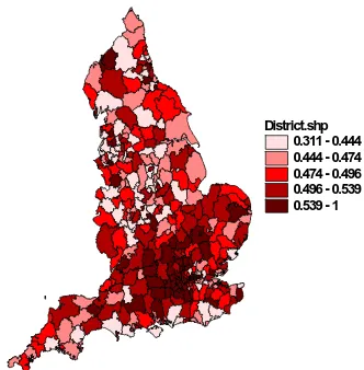
These κ values are illustrated in Figure 1, which suggests that labour is

relatively more efficient in the South East of England, although evidently there are

scattered pockets of ‘high efficiency’ elsewhere.

8

For simplicity, we do not control explicitly for separate covariates representing the causes of labour efficiency variations.

9

= 4.159, = 0.083, correlation observed and fitted values = 0.645

0

ˆ

b bˆ₁

10

District.shp 0.311 - 0.444 0.444 - 0.474 0.474 - 0.496 0.496 - 0.539 0.539 - 1

Figure 1 labour efficiency by UALAD

Iterative solution

Given an assumption of spatial equilibrium, it is assumed that the spatial

distribution of labour efficiency units (

κ λ

also given fixed numerical values for the exogenous terms T_Mir and σ , the solution to

equations (18…22) is obtained iteratively since there is no obvious analytical solution.

Iteration invariably solves the equations in the sense that after a number of iterations the

equations produce endogenous outcomes with steady-state values, at which point they are

terminated. Step 1 of the first round of iteration (t = 1) chooses initial wages per

efficiency unit of labour M_,0 i

w equal to 1 (and likewise ω) thus allowing an initial

estimate of house prices p_{i t,} (see below) hence π_{i t,} via equation (18). These then allow

calculation of (19), namely Yi t, . Step 3 uses these Yi t, values to obtain ,

M i t

w (20), using

also T_Mir and σ and the price index G_iM_,0, which is an initial guess of G = 1 for all

UALADs. The Fourth step of round 1 provides estimates of M_, i t

G (21) using M_, i t

w from

(20). The fifth step calculates ω using w_{i t}M_, and G_{i t}M_, as in (22).

For the second round of iteration11 (t = 2), given w_{i t}M_,−1 and the house price model

coefficients and variables we obtain p_{i t,} and use ω κ_{i t, 1− i} to give π_{i t,} . This then allows

11

(19),(20),(21) and (22) to be recalculated. In subsequent rounds of iteration (t = 3,…,T)

the same steps are applied, using the estimates of the preceding round for (18). The

iterations terminate when the values of the endogenous variables G_{i t}M_, ,w_{i t}M_, , π_{i t,} and

reach steady state. The stopping criterion giving T is when

,

i t Y

2 7

1 1 ( itM itM ) 0

i

G −G ₋ < −

∑

,

2 7

1

( M M )

it it i

w −w₋ < −

∑

1

( _{it it} ) 1

i

π π 7

0−

−

− <

∑

) 1 7

0 1 ( _{it it}

i

Y −Y ₋ < −

∑

Figure 2 Correlation surface

Estimating the elasticity of substitution and trade cost function

In order to carry out the preceding solution leading to equilibrium, we need to

of substitution). In the trade cost function, is the straight line distance measured in

miles/1000. The optimal values of

ir d

τ and σ are also obtained by an iterative search. For

any single combination of σ and τ values, we solve equations (18…22) and then

calculate the Pearson product moment correlation between

κ

wage levels. Figure 2 shows the correlation surface, based on a 10 x 10 matrix of

correlations obtained over a range of values of σ and τ , indicating that, approximately,

3.0

σ = and τ =3.5.

The house price model

a) specification

The specification is a simplified version of the house price model of

Fingleton(2008), taking account also of the work of Cheshire and Sheppard (2004) and

Gibbons and Machin(2003) among others. The model gives house prices12 p_j on the left

hand side via the reduced form from equilibrium housing supply and demand levels .

On the demand side, assume that q depends on income level which equals the sum

of income (observed wage levels times number of workers

j q

j

o j

c j

Y

j

w λ ) within j and income

weighted by commuting distance ( ) between employment in UALAD k and place of

residence j, summing across all R UALAD’s, so that

jk D

xp(

= −

(26) 1

e ,

R

k k

Y D w D

=

∑

c o

, k

δ λ_k 0

j j jk = j=k

Assigning a value δ =0.05 has the effect of giving approximately zero weight

beyond 100 miles. Note that with D_jk =0, j = k, income is not down-weighted by

within-area commuting distances. Assume also that demand for housing in j depends

12

negatively on j’s price level (pj) and is positively related to j’s amenity ( ). Other

unmodeled factors are represented by stochastic disturbances . A

that the relationship between prices and quantities is linear in natural logarithms

j A

2 1~iid(0, 1I

ω σ

1

j

) ssuming

, the

13

demand function is

0 1 2 3

lnq_j =a +a Y_jc+a A_j−a lnp +ω (27)

The supply function

0 1 2

lnq_j = +b b lnp_j+b O_j +ς (28)

j p

assumes that the level of housing supply increases with and with the stock of

properties ( ) and that other unmodeled effects are captured by the disturbance term

. j O 2 2 , I

~iid(0

ς σ )

Normalizing the supply function with respect to p thus

0 2

1 1 1

1

lnp_j lnq_j b b O_j b b b b₁

ς

= − − + (29)

and substituting for lnq_j gives

1[a0 1 2 3 1

ln p_j =c +a Y_jc a A_j a lnp_j ω] c₀ c O_{2 j} +ξ

iid

+ − + − −

j j

Simplifying this equation gives

0 1 2 3

2 ln

~ (0, )

c

j j j

j

p d d Y d A d O

I

ε

ε ϖ

= + + − +

(30)

b) Estimation

The price data14pjare the average 2001 selling prices (all property types) by

UALAD15, data which are provided by the UK’s Land Registry. Income by area (Y_r) is

13

This produces a better fit to the data that a linear relationship, gives a constant elasticity and avoids negative prices.

14

Data provided by the UK’s Land Registry. 15

taken to equal the local wage rate (w_ro) times the local employment level (λ_r). The

observed wages are taken from the results of the Office for National Statistics’ New

Earnings Survey, which is carried out annually by the UK’s Office of National Statistics.

These are workplace-based survey data of gross weekly pay for male and female

full-time workers irrespective of occupation. These and employment levels are available on

the NOMIS website (the Office for National Statistics’ on-line labour market statistics

database). The variable is normalised by dividing by the value for the City of London.

The variable O which is equal to the number of owner-occupier households reported in

the 1991 Census of Population

c r Y

p

16

. The level of amenity Aj is given by three separate

variables, the number of square km per household AS, the square of the distance of the

area from London AL, and the level of educational attainment AE (see Appendix), so that

the estimated model becomes

0 1 2 3 4 5

ln e e e AEj e ASj e ALj e Oj c

j = + Yj + + + − +εj (31)

16

c) Results

Table 1 gives the OLS and 2sls estimates of equation (24).

Table 1. Initial Estimates of house price models

Dependent variable

parameter est. t ratio parameter est. t ratio

OLS 2sls

Constant 5.4175 10.70 5.4343 5.55

C j

Y 0.0005957 13.77 0.0005847 12.97

O -0.000001253 -2.14 -0.000001245 -2.10

AE 1.6025 12.34 1.5993 6.36

AS 5.1859 7.00 5.1570 6.72

AL -0.000004310 -13.39 -0.000004340 -13.07

R2 , 2

R 0.703 0.7070

Standard Error 0.242 0.2403

Log likelihood 2.4471 ---

Residual correlation I = 19.41 Z = 18.42

Degrees of freedom 347 347

Notes : 2

R = Squared Correlation actual and fitted. For the OLS model we use the conventional R2_statistic.

I is the standardised value of Moran’s I statistic for residual spatial autocorrelation.

Z is the standardised value from the Anselin-Kelejian(1997) statistic for residual spatial autocorrelation with an endogenous variable (no spatial lag).

The spatial autocorrelation tests use the matrix W defined in the Appendix.

The instruments used in the 2sls and for the test of 2sls residual spatial autocorrelation comprise the exogenous variables (constant, O, ) and 46 county dummy variables (coded 1 if the UALAD was within a county, zero otherwise, and eliminating Tyne and Wear to avoid the dummy variable trap).

,

Fitting the model by OLS does not take account of the possibly endogenous

variables AS and . The 4th and 5th columns of Table 2 give the two-stage least squares

(2sls) estimates. The indication is that all the explanatory variables are significant and

appropriately signed and that endogeneity is not a significant problem. However there is

significant residual spatial autocorrelation, which may be a consequence of omitted

spatially autocorrelated regressors, in which case the parameter estimates may be biased.

C j

Y

d) Allowing spatial interaction

It is assumed that the significant residual spatial autocorrelation reported in Table

1 is a manifestation of demand and supply being displaced from where they would

otherwise be. If prices ‘nearby’ , at k, are relatively high compared with j prices, this

will push demand out from k into j . We refer to this as a displaced demand effect. We

model this by assuming that j’s demand is positively related to the weighted average of

neighbours’ prices, equal to the j’th cell of the vector , in which is a

weighting matrix based on distance.

1ln

W p W1

0 1 2 3 1

lnqj =a +a Yjc+a Aj−a lnpj+νW ln pj+ω (32)

Likewise, we envisage a displaced supply effect in which relatively high k prices

will pull supply out from j in to k. In other words relatively high neighbours’ prices

causes housing supply that would otherwise locate in j to locate instead in j’s

neighbours, thus giving a negative relationship between j’s housing supply and the

weighted average of neighbouring prices, hence 2ln

W p

j

0 1 2 2

lnq_j = +b b lnp_j+b O_j −ηW lnp +ς (33)

Normalizing the supply function with respect to p gives

0 2

2

1 1 1 1

1

ln p_j lnq_j b b O_j W lnp_j

b b b b b₁

η ς

= − − + − (34)

and substituting the quantity supplied by the quantity demanded q_jgives

3

c

1 0 1 2 3 1 0 2 2

in which Aj is a composite amenity variable. Simplifying by assuming that

, as defined in the Appendix, gives

1 2

W =W =W

0 1 2 3

ln j jkln k jc j j

k j

p ρ W p d d Y d A d O εj

≠

=

∑

j

(36)

Introducing the number of square km per household AS, the square of the distance of the

area from London AL, and the level of educational attainment AE (see Appendix) in place

of Aj gives

0 1 2 3 4 5

ln ln c

j jk k j Ej Sj Lj j

k j

p ρ W p d d Y d A d A d A d O ε

≠

=

∑

Or equivalently in matrix terms we have

1

ln p= −(I ρW) (− Xd+ε) (38)

in which X is an n by k matrix17, I is the n by n identity matrix, d is a k by 1 vector of

parameters, ρis a scalar parameter and the disturbances ε ~iid(0,τ2I) allow for

measurement error in the price variable and for other unmodeled effects with variance

2

τ .

17

Table 2. Estimates of house price models

Dependent variable _lnp

parameter est. t ratio parameter est. t ratio

ML 2sls

Constant -1.9792 -3.75 -2.6976 -1.40

c j

Y 0.0001948 5.20 0.0005752 14.65

O 0.000000071 0.17 -0.000000201 -0.36

AE 1.4102 14.60 1.8457 8.20

AS 3.5599 6.52 4.3583 6.33

AL -0.000001231 -4.20 -0.00000066 -0.79

ρ _{0.6960 18.16 0.6014 4.70}

R2 , 2

R 0.8413 0.8025

Standard Error 0.1769 0.2108

Log likelihood 96.5174 ---

Residual correlation LM = 1.336 Z = 1.371

Degrees of freedom 346 346

2

R = Squared Correlation actual and fitted. For the OLS model we use the conventional R2_statistic.

LM is distributed as chi-squared 1 under the null hypothesis of no residual spatial autocorrelation I is the standardised value of Moran’s I statistic for residual spatial autocorrelation.

Z is the standardised value from the Anselin-Kelejian(1997) statistic for residual spatial autocorrelation with a spatial lag. The spatial autocorrelation tests use the matrix W.

For 2sls, the endogenous variables are , AE and the spatial lag of house prices. The instruments are the exogenous variables, and

46 county dummies, and for the spatial lag we use the exogenous variables and their spatial lags obtained by multiplying by W. c

j

Y

Table 2 gives both ML18 and 2sls estimates for the model, although because ML takes account only of the endogeneity of the spatial lag, attention is focussed on the 2sls

18

estimates. These show that there is a significant spillover effect (ρ≠0), and that the

coefficient signs are as anticipated, with negative values housing supply (O) and distance

from London(AL ), although the 2sls estimates show that these variables are insignificant.

Eliminating these insignificant variables gives

0 1 2 3

ln _{j jk}ln _{k j}c _{Ej Sj}

k j

p ρ W p d d Y d A d A ε_j

≠

=

∑

Table 3. Estimates of house price models

Dependent variable lnp

parameter est. t ratio parameter est. t ratio

ML 2sls

Constant -2.9000 -6.37 -4.0608 -4.52

c j

Y 0.000201 5.21 0.0005769 14.31

AE 1.4429 14.67 1.9029 8.69

AS 2.6990 5.40 4.1849 6.54

ρ _{0.7610 23.79 0.6967 15.47}

R2 , 2

R 0.8353 0.7998

Standard Error 0.1805 0.2185

Log likelihood 85.4999 ---

Residual correlation LM = 1.807 Z = 1.166

Degrees of freedom 346 346

The estimates ρˆ,dˆgiven in Table 3 are used to calculate π_{i t,} (equation 18) via

1 ˆ

ˆ

ln pt (I ρW) (X dt )

−

in which Xt denotes the value of matrix X for the t’th iteration, which changes because

the second column is equal to

, 1

, 1

exp( )

R c

j t jk k k

k

M k t

Y δD

κ λ

= −

=

∑

(40)

Model outcomes

The outcomes for the endogenous variables are presented as maps of the 353

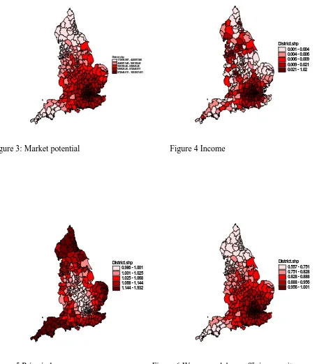
UALADs.Figure 3 shows the distribution of ‘market potential’ (equal19 to

1 1

, ( , )

M

r t r t Mir r

Y G σ−T −σ

∑

units and disposable income. It highlights the concentration in and around London and

the impact of inaccessibility to more peripheral UALADs. Figure 4 shows the income

distribution (equation 19), reflecting the large concentration of workers in cities, wage

levels and disposable income. Figure 5 shows the price index (equation 21), showing that

it costs more to gain the same level of utility in the peripheral areas, because of the ‘love

of variety’ which is more abundant in cities and their surrounds. Figure 6 gives the wage

per efficiency unit, which is a direct function of market potential. Figure 7 is the

observed wage level , which can be compared with the nominal wage level (Figure 8)

which is the endogenous model outcome equal to

o k w

r M r

w

κ

worker and Figure 10 is the house price given by exp(ln p_T)where

1

ˆ

ln p_T = −(I ρW) (− X d_T ˆ). Figure 11 is the observed house price distribution. Figure 12

shows the (model-based) price to wage ratio (π_{i T,} )indicating those areas (mainly in the

South East of England, but also in the rural South West and rural North) where under the

equilibrium assumption, disposable income is evidently greater than indicated by wage

rates. It also highlights those areas, particularly Northern industrial towns and remote

parts of Eastern England, where under the equilibrium assumption there is a paucity of

additional sources of disposable income and presumably high levels of debt.

19

District.shp 172896.881 - 424007.946 424007.946 - 568109.46 568109.46 - 699825.26 699825.26 - 872846.011 872846.011 - 1003037.651

District.shp 0.001 - 0.004 0.004 - 0.006 0.006 - 0.009 0.009 - 0.021 0.021 - 1.02

Figure 3: Market potential Figure 4 Income

District.shp 0.986 - 1.001 1.001 - 1.025 1.025 - 1.068 1.068 - 1.144 1.144 - 1.932

District.shp 0.557 - 0.751 0.751 - 0.828 0.828 - 0.888 0.888 - 0.956 0.956 - 1.001

District.shp 0.361 - 0.488 0.488 - 0.526 0.526 - 0.566 0.566 - 0.626 0.626 - 1.075

District.shp 0.258 - 0.345 0.345 - 0.384 0.384 - 0.428 0.428 - 0.486 0.486 - 1

Figure 7 Observed wages Figure 8 Nominal wage per worker

District.shp 0.147 - 0.315 0.315 - 0.363 0.363 - 0.41 0.41 - 0.476 0.476 - 1

District.shp 38966.174 - 72058.343 72058.343 - 88816.962 88816.962 - 112874.158 112874.158 - 284098.176 284098.176 - 2376715.833

District.shp

40703 - 89013 89013 - 129966 129966 - 176349 176349 - 274395 274395 - 639049

Residential property prices in England, 2001

District.shp 0.046 - 0.087 0.087 - 0.108 0.108 - 0.137 0.137 - 0.271 0.271 - 1.011

Figure 11 House prices Figure 12 House prices relative to real wages per worker

Simulation

To illustrate an application of the model, assume that employment falls by 10%

across all London UALADs, as shown by Figure 13. The model tells us that house prices

fall over a much wider area of the South East of England and by as much as 26% in

London (Figure 14 ) as a consequence of falling demand which is a combination of lower

wages and lower employment (equation 40), and also because of the externalities causing

house price changes to spill over to nearby UALADs. Wages depend on market potential

(equation 20) which is also negatively affected by the negative shock to employment.

Figure 15 shows the change in market potential relative to the City of London, which is

why in relative terms market potential change is positive as one moves away from

London. House prices in relation to real wages also more fall in and near London, giving

the positive differences20 shown by Figure 16.

20

District.shp -10 -10 - 0

District.shp -26.435 - -9.921 -9.921 - -0.44 -0.44 - 0.335 0.335 - 0.717 0.717 - 1.432

Figure 13 Employment change Figure 14 House price change

District.shp 0 - 0.767 0.767 - 2.545 2.545 - 4.605 4.605 - 7.051 7.051 - 9.123

District.shp -0.179 - 15.929 15.929 - 23.871 23.871 - 24.629 24.629 - 24.942 24.942 - 25.831

Figure 15 Market potential (rel. ch.) Figure 16 House price real wage ratio (rel. ch)

Conclusions

New economic geography theory is somewhat difficult to operationalize for

various reasons. One is that there are several exogenous unknowns, such as the elasticity

of substitution and the transport cost function. Another reason is the difficulty of deciding

which sector is under a monopolistic competition market structure and which sector is

competitive. While these operational decisions may be relatively easy in the international

context, when modelling small local urban economies as in this paper, any decision

seems somewhat more arbitrary. Also, at the level of cities, the price of property becomes

a major aspect of economic decision making, and the role of agriculture is minimal, and

while there is some literature which embodies the property sector within an NEG

framework, it does seems lacking in terms of the causal variables that typical have been

used to explain house price variation. Moreover, the basic theory as set out by FKV takes

a very simple view of the causes of wage level differences, and the assumption that

migration will lead to stable equilibria from a short-run equilibrium in which real wage

differences exist does not seem to accord with the reality of the urban economy, which is

for the UK at least essentially fairly static in terms of the long-run and stable patterns of

wage and price inequality, that do not seem to be moving towards a long run equilibrium,

but seem to be, approximately, in an equilibrium state already.

In this paper we endeavour to resolve some of the issues raised in attempting to

operationalize the FVK model in several ways. The paper first of all takes the radical step

of assuming that all firms are under monopolistic competition, with fixed costs and

internal increasing returns to scale. This seems to be a realistic first approximation to the

reality of the urban economy and has the benefit that with just one sector, the number of

exogenous parameters is reduced, and therefore we can proceed to use a simple numerical

technique to search for an optimum combination over a much reduced parameter space.

Secondly, we use a very simple method to adjust for labour efficiency variations across

space. Third, we do not treat the estimates obtained, with real wage differences across

space, as a short run equilibrium, but as a stable equilibrium defined by the equality of

the house price to disposable income ratio. Since house prices to real wages differ across

income differences exist and that these are quantifiable from the house price to real wage

ratios.

The paper illustrates the equilibrium outcomes for the model using data for

English local authority areas, and also gives the results of an small experiment in which

employment in London receives a strong negative shock, falling by 10%. The resulting

impact on house prices is strongly negative, not only in the immediate vicinity of the

shock, but also further afield because of the externalities and spatial interactions

embodied within the model.

.

References

Brakman, S, Garretsen, H, & M Schramm (2004) The Spatial Distribution Of Wages: Estimating The Helpman-Hanson Model For Germany, Journal Of Regional Science, 44 3 437–466

Cheshire P, Sheppard S (2004) Capitalising the Value of Free Schools: The Impact of Supply Constraints and Uncertainty, Economic Journal 114 499 F397-424

Fingleton, B (2008) Housing supply, housing demand, and affordability, Urban Studies 45 1545-1563

Gibbons S, Machin S (2003) Valuing English Primary Schools, Journal of Urban Economics 53 197-219

Glaeser E L (2008) Cities, Agglomeration, and Spatial Equilibrium, Oxford University Press, Oxford

Hanson, G H (2001) Scale Economies and the Geographic Concentration of Industry,

Journal of Economic Geography 1 255–276

Hanson, G H (2005) Market potential, increasing returns and geographic concentration,

Journal of International Economics 67 1 –24

Helpman, E (1998) The Size of Regions, in D. Pines, E. Sadka and I. Zilcha (eds.),

Appendix

A. Constructing the W matrix

The n by n matrix W is a row standardised version of matrix , Hence for cell

(j,k)

*

W

*

*

jk jk

jk k

W W

W

=

∑

with _jk* 1₂

jk

W d

= , in which djk is the straight line distance between locations j and k, and

for djk 50km. It seems reasonable to assume that the spillover does not

extend very far, since often market knowledge is localised and market conditions change

significantly with distance, so we approximate the localised interaction by assuming that

it only involves areas less than 50km apart and falls quite sharply as distance increases. *

0 jk

W = ≥

B. Educational Attainment

This is based on the 1998 key stage 2 tests taken by 11-year-old pupils initially available

for individual schools within smaller administrative areas nested within UALADs (these

are known as wards, of which there are 8413 in England). The mean scores per Ward

were then used to calculate mean scores for each of 353 English UALADs thus giving the