Formation and near-field dynamics of a wing tip vortex

(1)

Dynamics of a Wing Tip Vortex

Thesis by

Lavi R. Zuhal

In Partial Fulfillment of the Requirements for the Degree of Doctor of Philosophy

California Institute of Technology Pasadena, California

2001

(2)

11

(3)

Acknowledgments

At an age when most young men have entered the world to make their fortune, I struggled with mathematics, science and the mysteries of the natural world. Those were difficult days, but days that I will look back upon with fond memories. There are many people, too many to mention in these few paragraphs, who helped me to get to this point and succeed where others have failed. I would like to take this opportunity to thank some of the people who contributed most toward the completion of this thesis.

I would like to thank my advisor Prof. Morteza Gharib for giving me the

opportunity to work on this project. He gave me advice and direction while allowing me the freedom to develop the project according to my own vision. I would like to thank Profs. Hornung, Leonard, Shepherd, and Colonius for graciously agreeing to be members of my thesis committee. Their comments and suggestions were very helpful for making this thesis the "masterpiece" that you are about to read.

The many past and present members of Prof. Gharib's research group have lent their knowledge and experience in giving me many suggestions that saved hours and days of trial and error in perfecting the experimental setup and procedure. In particular, I would like to express my gratitude to Dr. Dana Dabiri, Dr. David Jeon, and Herm Dr. sc. techn. Heinrich Stiier.

I would like to thank the many friends who made my stay at Caltech almost bearable. My experience would not be complete without a well-balanced, daily meal from the Chandler Dining facility and "intellectual" conversations with my lunchtime companions Dr. Eric Burcsu, Dr. Sandeep Sane, Ioannis Chasiotis, and Benjamin Chow. Dr. Burcsu deserves special recognition for his continuous lunch attendance over the past five years.

Few people have had such a great influence on my personal and scientific

(4)

lV

(5)

Abstract

The search for a more efficient method to destroy aircraft trailing vortices requires a good understanding of the early development of the vortices. For that purpose, an experimental investigation has been conducted to study the formation and near-field dynamics of a wing tip vortex.

Two versions of the Digital Particle Image Velocimetry (DPIV) technique were used in the studies. Planar DPIV was used to obtain velocity fields adjacent to the wing surface. Stereoscopic DPIV, which allows instantaneous measurements of all three components of velocity within a planar slice, was used to measure velocity fields behind the wing. The trailing vortex was produced by a rectangular half-wing model with an NACA 0012 profile. All measurements were made at Reynolds number, based on chord length, of 9040.

(6)

VI

(7)

Table of Contents

ACKNOWLEDGMENTS ... III

ABSTRA. CT •.••...•••.••••••••••••••••••••••••••••••••••••••••••••••••••••••••••••••••••••••.•••••••••••••••••••.•..••••.••••••••••• V

TABLE OF CONTENTS ... VII LIST OF FIGURES ... X LIST OF TABLES ... XII LIST OF SYMBOLS ... XIII

INTRODUCTION ... 1

1.1 INTRODUCTION ... 1

1.2 REVIEWS ... 2

1.3 0BJECTfVES AND 0RGA IZATION OF THESIS ... 5

EXPERIMENTAL METHODS ... 8

2.1 INTRODUCTION ... 8

2.2 PLANARDPIV ... 9

2.3 STEREOSCOPIC PIV ... 10

2.4 IMPLEMENTATION ... 11

2.4.1 Planar DPIV ... 11

2.4.2 SPIV ... 11

EXPERIMENTAL SETUP ... 20

3.1 TESTING FACILITY ... 20

3.2 THE WING MODEL ... 20

3.3 SPIV SETUP ... 21

3.3.1 Light Sheet ... 22

3.3.2 Image Recording .............................................................. 23

3.3.3 Seeding ... 23

3.4 PLANAR DPIV SETUP ... 24

3-COMPONENT VELOCITY FIELDS BEHIND THE WING ... 29

4.1 I TRODUCTIO ... 29

4.2 EXPERIME TAL CONDITIO

s

..

.

...

.

..

.

...

.

...

.

...

.

...

..

.

..

.

...

.

...

.

..

.

29

4.3 AVERAGING METHODOLOGY ... 30

4.4 STEREOSCOPIC DPIV RESULTS ... 32

4.4.1 ZIC

=

0 ... 34

4.4.2. ZIC

=

1 ... 35

4.4.3 ZIC = 2 ... 36

4.4.4 Z/C

=

3 ... 36

4.4.5 ZIC = 4 ... 37

4.4.6 ZIC

=

5 ... 37

(8)

Vlll

5.1 INTRODUCTIO ... 56

5.2 CROSSFLOW PLANE PROFILES ... 57

5.2.1 Azimuthal Velocity Profile ........................................... 57

5.2.2 Axial Velocity Profile .................................................................. 58

5.2.3 Out-of-plane Vorticity Profile ... 60

5.3 CIRCULATION ... 61

5.4 CORE SIZE ... 65

5.5 COMPARISO WITH THEORY ... 67

5.6 SUMMARY ... 68

DYNAMICS OF THE WING TIP VORTEX ........... 82

6.1 INTRODUCTIO ... 82

6.2 AVERAGE AXIAL VORTICITY DISTRIBUTIO S ... 83

6.2.1 Vorticity Distributions at the Trailing Edge of the Wing .................. 83

6.2.2 Streamwise Evolution of the Wing Tip Vortex .................................... 84

6.2.3 Vortex Core Trajectory ........................................ 86

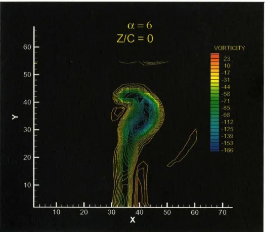
6.3 INSTANTANEOUS VORTICITY DISTRIBUTIONS ... 88

6. 3.1 Instantaneous Core Location ............................................. 91

6.4 SUMMARY ... 93

FORMATION OF THE WING TIP VORTEX ... 113

7.1 INTRODUCTIO ... 113

7.2 EXPERIME TAL CONDITIO

s .

.

...

.

..

.

...

..

...

.

....

..

....

.

..

.

...

..

...

..

113

7.3 VELOCITY AND VORTICITY FIELDS AROUND THE WING TIP ... 114

7.3.1 a=

rf

Case ... 115

7.3.2 a= 4° Case ... 117

7.4 SUMMARY ... 119

EFFECTS OF BOUNDARY LAYER AND TIP GEOMETRY ... 134

8.1 I TRODUCTION ... 134

8.2 EXPERIMENTAL CONDITIONS ... 135

8.2.1 Boundary Layer Modification ......................................... 135

8.2 2 Wing Tip Modifications ................................. 135

8.3 VORTICITY DISTRIBUTIO S ... 136 8.3.1 Boundary Layer Modification ....................... 136

8.3.2 Wing Tip Modification (Rounded Tip Geometry) .................... 138

8.3.3 Comparison Between Different Types of Wing Tip Geometry .................. 139

8.4 STRUCTURE OF THE VORTEX CORE ... 142

8.5 INSTANTANEOUS CORE LOCATION ... 144

8.6 SUMMARY ... ··· ... ··· ... 146

SUMMARY AND CONCLUSIONS ... 166

9.1 VELOCITY FIELD BEHIND THE WING ... 166

9.2 VORTICITY FIELD BEHIND THE WING ... 168

9.3 FLOW ADJACENT TO THE WING TIP ... 168

(9)

(10)

X

List of Figures

Figure 2.1. Photograph of Scheimpflug adaptor ... 16

Figure 2.2. Angular lens configuration ... 16

Figure 2.3. Calibration grid ... 17

Figure 2.4. Schematic for the SPIV 3-component reconstructions ... 1g Figure 3.1. Photograph of the setup ... 26

Figure 3.2. Light sheet optics ... 27

Figure 3.3. Schematic of planar DPIV setup ... 27

Figure 4.1. Schematic of the setup and the coordinate system ... 39

Figure 4.2. Running average vs. number of velocity fields ... 39

Figure 4.3. Average values computed with the two averaging methods ... 40

Figure 4.4. Three-component velocity field close to trailing edge of the wing ... 41

Figure 4.5. Velocity fields, zJc = 0, a= 0° ... 42

Figure 4.6. Velocity fields, zJc = 0, a= 2° ... 43

Figure 4.7. Velocity fields, zJc = 0, a= 10° ... 44

Figure 4.g. Velocity fields, zJc = 1, a= 2° ... 45

Figure 4.9. Velocity fields, zJc = 1, a= 1 0° ... 46

Figure 4.1 0. Velocity fields, z/c = 2, a= 2° ... 47

Figure 4.11. Velocity fields, z/c = 2, a= 1 0° ... 4g Figure 4.12. Velocity fields, z/c = 3, a= 2° ... 49

Figure 4.13. Velocity fields, z/c = 3, a= 10° ... 50

Figure 4.15. Velocity fields, z/c = 4, a= 1 0° ... 52

Figure 5 .1. Azimuthal velocity profile for a= 2° case ... 71

Figure 5.2. Azimuthal velocity profile for a= 4° case ... 71

Figure 5.4. Azimuthal velocity profile for a= go case ... 72

Figure 5.6. Axial velocity profile for a= 2° case ... 73

Figure 5.7. Axial velocity profile for a= 4° case ... 73

Figure 5.g. Axial velocity profile for a= 6° case ... 73

Figure 5.9. Axial velocity profile for a= go case ... 74

Figure 5.1 0. Axial velocity profile for a= 10° case ... 74

Figure 5.11. Out-of-plane vorticity profile for a= 2° case ... 75

Figure 5.14. Out-of-plane vorticity profile for a= go case ... 76

Figure 5.16. Peak vorticity vs. Z/C ... 76

Figure 5.17. Circulation vs. radius for a= 2° case ... 77

(11)

Figure 5.19. Circulation vs. radius for a = 6° case ... 77

Figure 5.22. Mean Ve vs. radius ... 79

Figure 5.23. Core radius vs. 2/C ... 79

Figure 5.24. Maximum Ve vs. 2/C ... 80

Figure 5.25. Minimum w vs. 2/C ... 80

Figure 5.26. Core radius vs. Z/C ... 80

Figure 6.1. Axial vorticity field, a= 0°, ZIC = 0 ... 94

Figure 6.2. Axial vorticity field, a= 2°, Z/C = 0 ... 94

Figure 6.6. Axial vorticity field, a= 10°, 2/C = 0 ... 96

Figure 6. 7. Axial vorticity fields at 2/C

=

0.5 ... 97

Figure 6.8. Axial vorticity fields at 2/C = 1 ... 98

Figure 6.9. Axial vorticity fields at 2/C = 1.5 ... 99

Figure 6.1 0. Axial vorticity fields at 2/C

=

2 ... 100

Figure 6.11. Axial vorticity fields at Z/C = 3 ... 101

Figure 6.12. Axial vorticity fields at Z/C = 4 ... 102

Figure 6.13. Average core trajectories ... 103

Figure 6.14. Instantaneous vorticity fields, a= 4°, Z/C = 0 ... 104

Figure 6.15. Instantaneous vorticity fields, a= 8°, 2/C = 0 ... 105

Figure 6.16. Instantaneous vorticity fields, a= 4°, Z/C = 4 ... 106

Figure 6.1 7. Instantaneous vorticity fields, a= 8°, Z/C = 4 ... 107 Figure 6.18. Instantaneous vorticity fields, a = 2°, Z/C = 3 ... 108 Figure 6.19. Instantaneous vorticity fields, a= 2°, 2/C = 3 ... 109

Figure 6.20. Instantaneous locations of the vortex core ... 11 0 Figure 6.21. Rms vs. Z/C ... 111

Figure 7 .1. Schematic of the experimental setup ... 121

Figure 7.2. Measurement plane locations for a= 0° case ... 121

Figure 7.3. Axial vorticity field, N = 1, a= 0° ... 122

Figure 7.8. Measurement plane locations for a= 4° case ... 127

Figure 8.l.a. Location ofthe trip wire ... 148

(12)

Xll

Figure 8.2. Boundary layer modification, axial vorticity field, a= 4°, Z/C = 0 ... 150

Figure 8.3. Boundary layer modification, axial vorticity field, a = 4°, Z/C = 1 ... 151

Figure 8.4. Boundary layer modification, axial vorticity field, a = 4°, Z/C = 2 ... 152

Figure 8.7. Tip geometry modification, axial vorticity field, a= 4°, Z/C = 0 ... 155

Figure 8.1 0. Tip geometry modification, axial vorticity field, a= 4°, ZIC = 3 ... 158

Figure 8.12. Comparison between different types of wing tip geometry ... 160

Figure 8.13. Generation of the vortices of opposite sign for a= 0° case ... 161

Figure 8.14. Comparison of the axial velocity profiles ... 162

Figure 8.15. Comparison of the circulation profiles ofthe main tip vortex ... 163

Figure 8.16. Instantaneous location of the vortex center for the three different cases .. 164

List of Tables

Table 5.1. Comparison of circulation at the trailing edge and the total circulation at ZJC = 4 .... 65

(13)

List of Symbols

a

AR

a

3-dimensional lift curve slope ( dC1/da)

aspect ratio

angle of attack

a1, a2, p~,

P

2

angles between the cameras and the interrogation plane

b

c

1

DPIV <p

r

v

,

Z/C=Q

N v (I) p Ptot r p

ravg

rrns

wmg span

chord length

lift coefficient

Digital Particle Image Velocirnetry

angle between the lens plane and the camera plane

circulation

wing tip vortex circulation at the trailing edge

lift per unit span

label for the streamwise location for measurement adjacent to the wing

viscosity

vorticity

pressure

total pressure

vortex core radius

density

average location of the vortex center

(14)

R

Re

T

e

u

Ve

w

X

y

z

ZIC

XIV

radial distance from the vortex center

Reynolds number

nondimensional time

angle between the object plane and the lens plane

freestream velocity

azimuthal velocity

out-of-plane velocity

lateral coordinate

vertical coordinate

longitudinal coordinate

(15)

Introduction

1. 1 Introduction

The dynamics of trailing vortices are of great importance in engineering. Trailing

vortices are produced at the tip of lifting surfaces where fluid accelerates from the

high-pressure to the low-pressure region. The interest in understanding the dynamics of

trailing vortices is motivated by the problems associated with their presence. One

problem associated with tip vortices is the noise generation on rotorcraft. Blade vortex

interaction has been identified as the major source of noise generated by a rotor. The

noise is generated when a blade passes over tip vortices produced by other blades.

Another problem is that of trailing vortices generated by aircraft wings. Large transport

aircrafts are known to produce strong and persistence trailing vortices. These vortices

induce rolling moments that can be hazardous to a following aircraft. The safety hazard

presented by the trailing vortices determines the spacing distance between aircrafts

during landing. This results in a limited number of airplanes that can land at an airport

within a certain period of time, which obviously has some economic impact.

For the reasons presented above, wing tip vortices have been the subject of many

investigations in the past. Most of the previous investigators focused their attention on

(16)

Introduction

of trailing vortices in the far field is reasonably well understood and documented. However, the formation and the near field dynamics of wing tip vortices have not been adequately studied.

In this thesis, results from an experimental study of formation and the near field dynamics of wing tip vortices are presented. The wing tip vortices are studied by using two versions of Digital Particle Image Velocirnetry (DPIV), which are non-intrusive global velocity measurements techniques. From the measured velocity fields, the formation, dynamics, and structure of the trailing vortex are examined.

1

.

2 Reviews

There are numerous publications found in the literature on the topics of wing tip vortices. In this section, we only review a few of those that are most relevant to the current study. Extensive reviews on the topics of wing tip vortices can be found in Widnall (197 5) and Spalart ( 1998).

Measurements of velocity profiles have been attempted by many researchers in the past. Logan (1971) measured both azimuthal and axial velocity profiles by using five-hole pressure probes. He found that there is significant retardation of axial velocity within the vortex core over the downstream distance of 10-26 chord lengths behind the wing. Logan also reported that there is axial velocity excess at the edge of the vortex core. Baker et al. (1974) made a series of LDV measurements of the trailing vortex. They considered the effect of vortex meandering in the data analysis. Baker et al. (1974) reported that the vortex meandering reduced the maximum tangential velocity by

approximately 30%. They also found that the measurements are in reasonable agreement

(17)

with the theory of Moore and Saffman. Bippes ( 1977) studied the tip vortex by means of

hydrogen bubble method for flow visualization and photo-grammetric evaluation of

photographs. From the results, Bippes concluded that the direction of the axial flow in the core depends on the Reynolds number. Green and Acosta (1991) performed trailing

vortex measurements by using a double-pulsed holographic of injected micro bubbles.

They found that the core mean axial velocity is consistently higher than the freestream velocity in the region close to the wing. Additionally, they found that the axial flow is

highly unsteady. They also concluded that the axial velocity strongly depends on the Reynolds number (similar to Bippes conclusion). Devenport et al. (1996) examined the

structure of wing tip vortices by using hot wire anemometry. They developed a theory to correct for the effects of vortex meandering. However, as mentioned in Spalart (1998),

their strategy to correct the meandering effect is not definitive.

Almost all measurements mentioned in the above paragraph are performed by using either intrusive or point measurement techniques. However, it is well known that the wing tip vortex is very sensitive to disturbances from intrusive probes and can become subjected to a meandering motion. These problems can be resolved by

employing the particle image velocimetry (PIV) technique. (The measurement technique employed by Green and Acosta is actually a primitive version of this.) A number of PIV

measurements of the wing tip vortex have been conducted in the past. Vogt et al. ( 1996) used planar DPIV to measure wing tip vortex shed by an NACA 0012 wing. From the PIV measurements, they obtained azimuthal velocity profiles across the vortex core and

showed that the profile looks different from LDV measurement results. Jacob et al.

(18)

Introduction

wing) up to a 1400 chord-length downstream by using planar DPIV. Their results

showed that the maximum tangential velocity varies very little near the wing and decays

in the region far from the wing. Recently, Chen et al. (1999) studied the wake of a

flapped wing using planar DPIV. Their results showed that trailing vortices of a flapped

wing exhibit Lamb-Oseen tangential velocity distribution with slow growth.

4

The existence of axial flow within the core of tip vortices was investigated

analytically by several researchers. Batchelor (1964) showed that the axial flow in the

core is a consequence of the low-pressure region within that core, which accelerates

fluids in the core region faster than the freestream velocity (assuming that the flow is

steady and the viscous effect can be neglected). He also gave a similarity solution for the

flow in the far downstream. Moore and Saffrnan (1973) studied the structure of laminar

trailing vortices by including the effect of core viscosity. They showed that the axial

flow within the vortex core could be either higher or lower than the freestream velocity,

depending on the distribution of tip loading on the wing. Both Batchelor's and

Moore-Saffrnan's analyses are based on the assumption that the perturbation of the axial velocity

within the core is very small.

The formation and early development of wing tip vortices have not been studied

sufficiently. Part of the problem is that the flow is highly three-dimensional in the region

near the wing, which makes it difficult to study this problem experimentally. Francis and

Kennedy (1979) provide one of a few experimental studies on the formation of a trailing

vortex. Francis and Kennedy investigated the formation of a wing tip vortex by using hot

wire anemometry. They took velocity measurements close to the wing surface and

(19)

measurements. Green ( 1988) performed a surface flow visualization to study the early stages of the vortex roll up process. Several numerical simulations to model the roll up of wing tip vortices have been performed in the past. The most common procedure is to replace the vorticity in the wake with a vortex sheet and study the evolution of the vortex

sheet. Moore (197 4) studied the roll up of vorticity shed by an elliptically loaded wing.

Krasny (1987) numerically investigated the vortex sheet evolution for an elliptically loaded wing and a configuration that includes flap and fuselage.

1.3 Objectives and Organization of Thesis

The ultimate goal of research on wing tip vortices is to find a method that can accelerate the "destruction" of the trailing vortices. In real situations, trailing vortices

generated by an aircraft normally undergo the so-called Crow instability (Crow 1970).

This sinusoidal instability is caused by the interaction of the two trailing vortices

generated by the wing. By this instability, the two vortices eventually touch each other and break into a series of vortex rings. The destruction of tip vortices by the Crow instability is more rapid than the viscous or turbulent decay of a single vortex (Widnall

1975). However, the destruction process by this instability is not very efficient since the instability grows very slowly. The search for another mechanism, which would lead to a more efficient way of eliminating trailing vortices, requires a good understanding of the early development of the vortices. Unfortunately, the early stages of the development of a wing tip vortex are still not well understood.

(20)

Introduction

measurements using two versions of the Digital Particle Image Velocimetry technique.

From the velocity measurements, the following can be studied and addressed:

1. The structure of the trailing vortex with the correction for the meandering effect.

2. The formation of the trailing vortex starting from its early stages on the wing

surface.

3. The interaction between vortices shed by the wing and its effect on the motion of

the trailing vortex.

4. The effect of wing tip geometry and the boundary layer on the strength and

motion of the wing tip vortex.

6

The thesis is organized into nine chapters. The basic descriptions and implementation

of the two versions of the PIV method used in the experiments are discussed in Chapter

2. The description of the apparatus used during the experimental phase is given in

Chapter 3. The 3-components planar velocity fields, measured using stereoscopic PIV,

are presented in Chapter 4. The structure of the measured wing tip vortex is considered

in Chapter 5. In Chapter 6, the trailing vortex dynamics and vortex interactions behind

the wing are examined. Results from velocity measurements around the wing surface are

presented in Chapter 7. The effects of boundary layer and tip geometry are studied in

(21)

CHAPTER2

Experimental Methods

2.

1 Int

r

od

u

ct

i

on

It has been reported in the literature that there were various problems encountered by the previous researchers in conducting velocity measurements of wing tip vortices. Some of the problems encountered are the following:

1. The vortices are very sensitive to disturbances from intrusive probes. 2. The locations of the vortices are changing with time even in the steady

conditions of the wind/water tunnels (vortex meandering phenomenon). 3. The flow is highly three-dimensional especially in the near field region.

These facts of course affect the choice of experimental methods used in the present study. A measurement technique such as three-component laser-Doppler velocimetry (LDV) can guarantee no disturbance of the flow with high spatial and temporal resolution. However, vortex meandering phenomenon makes it difficult, if not

impossible, to study this problem using pointwise measurement techniques. In addition, single-point diagnostic tools also require measurements at many locations within the vortex. This prevents instantaneous measurements of the whole region of study.

(22)

Experimental Methods

9

techniques that satisfies the requirements mentioned above. Digital particle image

velocimetry (DPIV) is a technique capable of measuring two-component velocity field

within a plane instantaneously. To address the three-dimensionality of the flow,

three-component velocity measurements are preferred. There are several techniques, extended

versions of DPIV, which allow instantaneous measurement of a three-component

"planar" velocity field. One of these techniques is stereoscopic PIV (SPIV). Both DPIV

and SPIV are used in the present study.

In the rest of this chapter, brief descriptions of DPIV and SPIV are given. The

implementations of both methods in the present study are discussed.

2.2 Planar DPIV

In PIV, small and neutrally buoyant particles are added to the flow. The region of

study is illuminated twice with a light sheet, generated by high-powered lasers. It is

assumed that the particles move with the flow velocity between the two illuminations.

The light scattered by the tracer particles during the two illuminations are focused onto

two separate frames of a CCD sensor that is positioned parallel to the light sheet. The

images are then acquired in real time and downloaded to the hard disk of a computer.

The projection of the local displacement vectors of the particles onto the plane of

the light sheet is measured by cross-correlating the two sequential images. The image

interrogation scheme used to obtain the displacement field is described in Willert and

Gharib (1991). The velocity field is obtained by taking into account the time between

(23)

quantities such as circulation, stream functions, and vorticity components normal to the

plane of the light sheet can be numerically computed.

2. 3 Stereoscopic PIV

In stereoscopic PIV, one measures three-component velocity field within a plane

instantaneously. Among several other three-component PIV methods existing in the

literature, SPIV was chosen in the present study because it is a direct extension of planar

DPIV. The image interrogation scheme used in this technique is exactly the same as that

use in planar DPIV.

The planar-three-component velocity field is obtained by comparing the in-plane

displacement field as viewed by two cameras, placed at different locations, which are

focused onto the same region in the flow. The in-plane displacement field as viewed by each camera is obtained by using the same routine as that used in planar DPIV.

Besides being a direct extension of planar DPIV, SPIV also has another advantage

in the present experiment. The fact that SPIV takes into account the out-of-plane motion

(which is ignored in 2D DPIV) can improve the accuracy of the in-plane motion. This is of course an advantage especially in the present experiment where there are large

out-of-plane motions.

The fact that SPIV only provides measurement of all three velocity components

within a plane implies that it has no advantage over 2D DPIV in giving additional

vorticity components. Only in-plane velocity gradients are available from the measured

velocity field. Consequently, the only vorticity component that can be calculated from

(24)

Experimental Met

h

o

d

s

11

vorticity components is certainly desirable, having only one vorticity component is not a drawback since the out-of-plane vorticity is the main vorticity component in the problem currently studied.

2

.

4 Implementation

2.4.1 Planar DPIV

The implementation of planar DPIV in this experiment is very similar to that described in Vogt et al. ( 1996). The light sheet is aligned perpendicular to the free stream direction. The only modification is the placement of the recording camera. Instead of mounting the camera inside the tunnel with the optical axis perpendicular to the light sheet, the camera is placed outside the test section wall of the wind tunnel. The light, scattered by the seeding particles, is directed into the camera by a small 45-degree mirror placed inside the wind tunnel. The mirror is mounted far enough downstream from the measurement plane to reduce the effect of flow disturbance due to its presence. A more detailed description of the planar DPIV setup is given in Chapter 3.

The placement of the small mirror instead of the camera inside the wind tunnel reduces the interference. Also, this arrangement prevents the contamination of the CCD chip by the smoke particles.

2.4.2 SPIV

(25)

described in this subsection. A more detailed description of SPIV can be found in Raffel,

Willert and Kompenhans (1998).

In SPIV, stereoscopic recording is achieved by the use of a second camera, which records images of particles in the region of interest from a different viewing axis. The measurement precision of the out-of-plane component increases as the opening angle between the two cameras reaches 90 degrees (Raffel, Willert and Kompenhans, 1998). There are two basic stereoscopic imaging configurations available: a lens translation method and an angular lens displacement method. The latter was chosen in this experiment since it is more robust than the former.

In the angular lens configuration, the lens principal axis is aligned with the principal viewing direction. However, with this approach, it is impossible to get focused across the entire field of view since the object plane is no longer perpendicular to the axis of the lens. This problem can be overcome by tilting the CCD plane according to the Scheimpflug criterion. The Scheimpflug criterion says essentially that the object, lens,

and image plane of each camera intersect at a common line.

In the present experiment, the Scheimpflug condition is accomplished with the help of Scheimpflug adaptors. Figure 2.1 shows the photograph of one of the

Scheimpflug adaptors used in the experiment. As shown in Figure 2.1, the lens is fixed at some distance from the camera head. The camera is mounted on an aluminum box that can be rotated with respect to the lens. The procedure of focusing the cameras according to the Scheimpflug condition is as follows. First, each adaptor is aligned to the

(26)

Experimental Methods

13

camera is tilted until the whole field of view is focused. After completing the last step,

the viewing direction of each camera has changed slightly. Therefore, it is necessary to

re-align the lens and repeat the whole procedure until both cameras image the same

measurement area with focus across the entire field of view. This iterative process can be

quite time-consuming.

The process of tilting the CCD plane with respect to the lens plane introduces

another problem. By tilting the camera head, the magnification factor is no longer

constant across the entire field of view since, for each camera, one side ofthe object

plane is closer to the principal axis of the lens than the other side of the object plane (see

Figure 2.2). This results in a strong perspective distortion that requires an additional

calibration.

To calibrate the cameras, a square calibration grid is placed inside the light sheet.

The top part of Figure 2.3 shows a typical image of the grid from one of the cameras. As

depicted in the figure, the horizontal lines, especially on the top and bottom part of the

images, are highly distorted. Trapezoids are formed instead of rectangles due to this

perspective distortion. "Dewarping" the original images from each of the camera so that

the magnification factor remains constant over the entire image can solve this problem.

The dewarping process consists of fmding a mapping function for each of the cameras

that maps the trapezoids into rectangles of the same size. The detailed steps are as

follows:

1. Locating the grid intersections by cross-correlating the image with a

+

correlation mask. The peaks of the cross-correlation are identified as the

(27)

2. Selecting an origin that is a common point in images from both cameras.

3. Setting the spacing between the grid lines and reconstructing a rectangular

grid.

4. Finding the mapping function, for each camera, which maps the original image to that of the reconstructed rectangular grid.

5. Applying the mapping to each particle image obtained by the corresponding

cameras.

The bottom part of Figure 2.3 shows the image of the grid after applying the mapping to

the original image (upper part of2.3). It is clearly shown that the "trapezoids" have been transformed into "rectangles". Note that some portions of the image on the upper and lower edges are lost in the transformation process.

Once the original images are dewarped, image pairs from each of the cameras separately undergo standard DPIV image interrogation schemes to obtain two projected, planar displacement fields.

The three-dimensional displacement field is reconstructed from the two planar

displacements fields. Figure 2.4 shows the general geometric description used for the

reconstruction. In a coordinate system center at the origin (point 0), camera 1 and

camera 2 are located at points (x~, y1, z1) and (x2, y2, z2), respectively. Consider point Q,

somewhere in the object plane, where the displacement vector is to be determined. Angle

a

1 is defined to be the angle between the viewing direction of camera 1 and the z

direction in the XZ plane while

P

1 is that in the YZ plane. Similar definitions can be

(28)

Experimental Methods

15

From the schematics shown on the lower part of Figure 2.4, it is easy to see that

the three displacements can be reconstructed by using the following formulas (Willert

1997):

dx = dx₂tan

a

,

-

dx, tan a₂

tan

a,

-tan

a

₂ (2-1)

dy = dy2 tan/31 -dy1 tan/32 tan /31 - tan

/3

2

dz = dx2 -dxl

tan

a, -

tan

a

₂

Using (2-3), the expression for dy can be rewritten:

dy= dy, +dy2

+

dx2 -dx1 (tan/32 -tan/31) . 2 2 tan

a

₁-tan

a

₂

(2-2)

(2-3)

(2-4)

Note that (2-4) can be used, instead of (2-2) in the case where ~1 and ~2 are very small, as

in the present experiment.

The formulas for reconstructing the 3-component displacements from the planar

fields given above assume that the angular difference along the vector dx, the

displacement vector, is negligible. Therefore, these formulas are good as long as the

distance between the light sheet and each of the cameras is large, as is the case in this

(29)

Figure 2.1. Photograph of Scheimpflug adaptor

[image:29.540.124.415.85.321.2] [image:29.540.71.457.457.663.2]

Object

Figure 2.2. Angular lens configuration

...

,,,

... ,

'

' ...

\ _\_\

',/

_'... _.

\ \

(30)

Experimental Methods

17

(31)

To camera 1

...

/ />.,P 0 ·· ... .

dXt

:

>:

I I

A

i

l

dx :~

l

I I :

To camera 2

1

---dy,

~~r{

(32)

(33)

CHAPTE

R

3

Experimental Setup

3

.

1 Testing Facility

The experiments were conducted in the GALCIT 2-foot wind tunnel. The tunnel,

which is a low-turbulence closed-loop wind tunnel, has a test section of two feet wide,

two feet high, and seven feet long. The sidewalls and the ceiling of the tunnel are made

of 1.8 em thick clear Plexiglas. The floor is made of plywood. The tunnel can be

operated up to a maximum speed of 50 m/s.

3.2 The Wing Model

The wing model has an NACA 0012 profile with an effective span of 41.91 em

and a chord length of 9.1 em. The tip of the wing model is rectangular.

The wing is made from composite material. However, the composite material

resulted in unwanted reflections of the light sheet when taking measurements close to or

around the surface of the wing. Painting the wing with ultra flat black color reduced the

unwanted reflections allowing measurements to be made in the region very close to the

wing. However, light still scattered from the tip surface when the light sheet impinged on

(34)

Experimental Setup

problem is finally solved by putting an NACA 00 12-shape mirror on the surface of the

tip. The mirror reflects the light uniformly back up onto the light sheet, ultimately

eliminating the unwanted reflections.

The wing is positioned vertically at 40 em behind the front of the test section. It

is mounted on a force balance that is located underneath the test section. The force

balance is placed on a rotating table. The angle of attack of the wing is adjusted by

turning a wheel on the rotating table. The mounting system is designed such that the

wing would remain near the center of the test section regardless of the angle of attack.

Figure 3.1 shows the photograph of the whole experimental setup.

3.3 SPIV Setup

21

A photograph of the SPIV setup can also be seen in Figure 3 .1. The whole SPIV

system is mounted on a frame which is connected to a railing system that is fixed to the

floor of the room. The frame consists of two legs, one on each side of the tunnel, and two

sets of beams that bridge the two legs. Each of the two cameras is installed on each of

the two legs. As shown in the figure, the laser and the light sheet optics are mounted on

the upper bridge. The light generated is deflected down into the tunnel so that it is

aligned perpendicular to the flow direction.

The frame can be moved parallel to the tunnel to take data at different

downstream stations. Notice that in this arrangement, the distance between the light

sheet and the cameras is always fixed. Therefore, cameras, as described in the last

(35)

re-calibration when the light sheet is moved to a different downstream station since the light

sheet and the cameras move together.

3.3.1 Light Sheet

The light source for the light sheet is provided by a New Wave Research "Gemini

PN" 120 mj/pulse Nd:Yag laser. The laser system consists of two IR laser heads

combined in a single package. Each is operated at 15 Hz with pulse duration of 10 ns,

which matches the framing rate of the cameras.

Figure 3.2 shows the schematic of the light sheet optics. The optics consists of

two spherical and two cylindrical lenses. This combination of lenses allows for the width

and the thickness of the light sheet to be changed independently. The thickness of the

light sheet is approximately constant across the field of view. After passing the light

sheet optics, the light is deflected down perpendicularly using a 45-degree mirror.

In this experiment, the light sheet is aligned perpendicular to the direction of the

free stream. In this arrangement, the out-of-plane particle loss can be significant. One

method to reduce the loss is to reduce the time between the first and the second image

recording. This, however, reduces the dynamic range in the measurement. The method

used in this experiment to reduce the out-of-plane loss is to shift the light sheet slightly,

in the downstream direction, between illumination pulses. Moreover, the light sheet is

slightly thickened to accommodate strong out-of-plane gradients in the vortex core

(36)

Experimental Setup

3.3.2 Image Recording

The flow is imaged using two Pulnix TM-970 1 CCD cameras (768x480 pixels).

105 mm focal-length lenses are mounted in front of the cameras on the Scheimpflug

adaptors. The synchronization of the two cameras is achieved using an external master

triggering device (Sigma Electronics CSG-4500) that sends a synchronization signal to

the two cameras.

23

The output signal from one of the cameras is used to trigger the laser system

through a timing box. The timing box in tum controls the flash lamp signal of the lasers.

For all measurements in this experiment, the time delay between images in a pair is set at

650 !lS.

The output signals from the cameras are recorded on a real-time digital recorder.

The signals are digitized using a color analog-to-digital frame grabber (Coreco RGB-SE),

which acquires images at resolution of 640x480 pixels. The digitized images are then

downloaded to a hard disk and processed by SPIV software.

3.3.3 Seeding

Choosing proper tracer particles for PIV measurements in wind tunnel

applications is a difficult task. Particles that are often used for wind tunnel measurements

are not easy to handle. Liquid droplets tend to evaporate quickly and solid particles are

difficult to disperse (Raffel et al., 1998). There is also concern about whether the

particles scatter enough light.

The first tracer particles used in this experiment are generated by pressurizing

(37)

much denser than air, they have low particle distributions inside the vortex core. The

particle concentration was so low that a hole could be observed by the naked eye in the

low-pressure region (vortex core).

The final choice for particle seeding was smoke generated by the CORONA

COLT 4 smoke generator. The machine produces particles that range in size from O.lp

to 0.5p in diameter. This type of tracer particle is able to scatter enough light, which

resolves the problem of low particle concentration in the vortex core.

3.4 Planar DPIV Setup

Planar DPIV is used in this experiment to take velocity measurements around the

tip of the wing. Views of the cameras are partly blocked due to the presence of the wing.

Therefore, SPIV, in the present setup, can only be used to take measurements in the

region above the wing tip. (Again, the wing is mounted vertically so that above the wing

tip means farther away from the wing in the spanwise direction.) It is possible to change

the setup by moving the wing model farther downstream and arranging the camera

differently. However, that requires changing the whole experimental setup.

Alternatively, measurement can be made in this region easily by using planar DPIV,

which only requires a slight change in the setup.

The light sheet optics and image recording equipment are exactly those used for

SPIV. Here, only one of the cameras is needed. The camera is mounted outside the

tunnel (mounted on the same frame discussed in 3.3) with the viewing axis perpendicular

to the sidewall of the tunnel. A small mirror is mounted inside the tunnel to direct the

(38)

Experimental Setup

mirror is mounted far enough downstream to reduce the interference effect. The

schematic of the planar DPIV setup is shown in Figure 3.3.

(39)

(40)

Experimental Setup

LASER

u

Spherical F =250mm

Cylindrical F=60mm

•

1----lt--{}---{}{}---~or

t

I

_I

Spherical

F= -150mrn

Cylindrical

F=80mm

Figure 3.2. Light sheet optics (side view)

Side wall of the wind tunnel I

/ Light Sheet

('~ I I I I I I I I

L...-..->

~

...

~---Mirror

I ~ \ : :

'

'w;,,

I

Q----

C•m•"

Figure 3.3. Schematic of planar DPIV setup (top view)

(41)

(42)

CHAPTE

R

4

3-Component Velocity Fields

Behind the Wing

4

.

1 Introduction

In this chapter, we present the majority of PIV data obtained in the experiment.

The experimental conditions are given in Section 4.2. This is followed by discussion

about the methods of averaging used to obtain average velocity data Lastly, the

three-component planar velocity fields, measured by SPIV, are presented in Section 4.4. The

results presented in this chapter will be discussed in detail in Chapters 5 and 6.

4.2 Experimental Conditions

The coordinate system used throughout the rest of this thesis is shown in Figure

4. I. The Z-axis is parallel to the freestream direction. The Y -axis is along the span and

the X-axis forms a right-handed system with the Z andY-axis. With this coordinate

29

system, the measurement plane is in the X-Y plane. The area at which the measurements

are made is also depicted in Figure 4.1.

For all data taken in this experiment, the freestream velocity of the wind tunnel is

set at 1.5 rnls. This corresponds to a Reynolds number, based on the chord length of the

(43)

reduce the out-of-plane particle loss described in Chapter 3. There have been several attempts to increase the freestream velocity. The results are not very encouraging even with the combination of increased light sheet thickness and the light sheet stepping

method described in the last chapter.

For SPIV measurements, data is taken at different angles of attack, ranging from

0° to 10° with 2° increments. For each angle of attack, measurements are made at

different downstream stations, ranging from 0 to 5-chord lengths behind the wing.

For all measurements, 200 pairs of images are taken for a given angle of attack at

a given streamwise location. This corresponds to 200 instantaneous velocity fields for

each case. Figure 4.2 shows the plot of the number of instantaneous velocity fields against the running average of the in-plane velocity components along with their rrns

fluctuations at a given point in the field (somewhere in the vortex core). It is clearly shown in the figure that the running averages of these quantities converge at ''Number of

fields" equals 200.

4.3 Averaging Methodology

Average quantities presented in subsequent chapters are calculated from ensemble

average velocity fields. It is found that, in some cases, the location of the wing tip vortex fluctuates in space, a phenomena referred to as "vortex meandering". Because of the

unsteadiness of the vortex location, the values of the average quantities depend on the

way the averaging is done.

There are two methods used to compute the ensemble average of the velocity

(44)

3-Component Velocity Fields

Behind

the Wing

31

fields and compute the ensemble average. The second one is to identify the center of the

vortex in each instantaneous field, shift the individual field so that the vortex center is

located at a common point, and then compute the average.

Near the trailing edge, the main vortices are approximately steady. In this region,

the average velocity is calculated using the first method. It will be shown in the

subsequent chapter that the wing tip vortex meanders in regions downstream of the wing.

In these cases, the second method is employed to compute the average.

Figure 4.3 shows the profiles of azimuthal velocity, axial velocity, and vorticity

along a cut through the center of the vortex. These profiles are taken from mean velocity

fields calculated by the two methods discussed previously. The figure shows that, while

in most regions the profiles are almost identical, the peak values of the profiles calculated

by the second method are higher than those computed by the first method. The difference

in the values of the peak vorticity, for example, is approximately 5%. Also, the peak

value of the mean out-of-plane velocity computed by the first method is approximately

3% lower than that computed by the second method. This is due to the vortex

unsteadiness that smears out the peak values when averaging is computed using the first

method.

Although the differences in the peak values calculated by the two methods are

relatively small for the example presented above, they are not always the case in general.

The difference in peak values as high as 10% is observed in some of the data. In addition

to the smearing out of the mean peak values, vortex meandering also generates

fluctuations of velocities at a given point fixed in space. These fluctuations are

(45)

of global instantaneous measurement technique in the present studies is clearly an advantage since it allows a definitive correction for the vortex meandering effect.

4

.

4 Stereoscopic DPIV Results

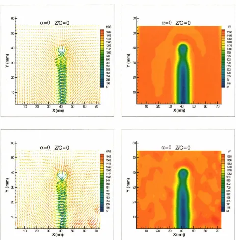
In this section, results from stereoscopic PlY measurements are presented. As a reminder, stereoscopic PlY is used, in the present experiment, to measure velocity fields downstream of the wing (0-5 chord-length behind the wing). Also, the wing is mounted along the Y -axis and the location of the tip, at a 0° angle of attack, is at coordinate point ( 41, 40. 5), in all plots to follow. The unit for distance and velocity is mm and rnrnls, respectively.

Figure 4.4 presents a typical component planar velocity field in three-dimensional space measured at the trailing edge of the wing using stereoscopic PlY. For clarity of the velocity vectors within the vortex and its core, the freestream velocity is subtracted (the out-of-plane component of velocity in the figure is relative to the

freestream). In the figure, both the colorbar legend and the size of the arrows indicate the magnitude of the velocity vectors. Besides the obvious in-plane motion, this figure depicts the presence of axial velocity in the vortex core and wake region. In this frame of reference, the axial velocity vectors are directed toward the wing, indicating that the out-of-plane velocities within the vortex are lower than the freestream velocity.

(46)

3-Component Velocity Fields

Behind

the Wing

differently in the rest of this section. For each case, the in-plane motion is presented in

the vector field format while the out-of-plane component is displayed as a contour plot.

33

For each case (given angle of attack, at a given streamwise location), both the

average and one instantaneous field are presented. Again, the average is computed from

200 instantaneous fields, using methods described in Section 4.3 (the first method for

fields measured at 0 chord length and the second method for fields measured at 1-5 chord

length downstream of the wing).

All velocities are given with respect to a lab-fixed coordinate system. The

colorbar legend for the in-plane vector field is the magnitude of the total velocity (all

three components). This also means that the color bar legend for the vector field is

proportional to the pressure difference (P101-P). The color bar legend for the contour plot,

however, is with respect to the out-of-plane velocity magnitude only.

Note that the light sheet is always normal to the freestream velocity direction, not

normal to the wing tip vortex itself. Therefore, the measured velocity components are the

projections into this plane. This is important to note especially for high angle of attack

data taken in regions close to the wing where the normal direction of the vortex is not

exactly parallel to the Z-axis.

In this section, we present only the results of the measurements for a= 0°, a= 2°,

and a = 10° case. The last two cases represent the low (a = 2° and a = 4 ~ and high (a=

6° to a= 1 0°) angles of attack, respectively. Discussion about the results and possible

(47)

4.4.1 Z/C

=

0

In this subsection, we present velocity measurements taken at the trailing edge of

the wing (Z/C

=

0). The velocity fields, taken at this streamwise station, are shown in

Figure 4.5 to Figure 4.7 (the plots are arranged in order of increasing angle of attack).

Both instantaneous and average in-plane velocity components for a= 0° case

(left-hand side of Figure 4.5) show vectors, in the region near the wing, pointing toward

the root of the wing (inboard). At a= 0°, the flow behind the wing is just the wake flow

behind a slender body, as clearly depicted in the plots. At a very low angle of attack (a=

2~, the initiation of the tip vortex is clearly visible (see Figure 4.6). The directions of

in-plane velocity vectors on the high-pressure side are split. Near the tip, the vectors are

directed outboard circling the tip while vectors slightly inboard are still pointing toward

the root, as in the a

=

0° case. As expected, the tip vortex gets stronger as the angle of

attack is increased to a higher value (Figure 4. 7, for a= 10° case). Here, the pressure

side in-plane motion is directed toward the outboard part of the wing across the entire

field of view. For all a, vectors in the suction side are directed toward the root. The

presence of a shear layer at the trailing edge of the wing is evident in all in-plane vector

fields presented in this subsection.

Contours of average and instantaneous out-of-plane velocity components are

shown on the right-hand side of Figure 4.5 to Figure 4.7. Areas of very low out-of-plane

velocity are apparent in the wake region for a= 0° case (Figure 4.5). The out-of-plane

velocity increases in all directions away from the wake and approaches the freestream

velocity in the region far from the wing. At a= 2° (Figure 4.6), areas of very low axial

(48)

3-Component Velocity Fields Behind the Wing

35

low velocity continues to increase as

a

is increased further (as depicted in Figure 4. 7). However, the magnitude of the out-of-plane velocity is slightly higher (closer to

freestream value) than in the lower angle of attack case. This is understandable since at a higher angle of attack the out-of-plane direction (Z-axis) is no longer parallel to the normal plane of the vortex, especially in a streamwise location that is very close to the wing. The values, shown in the figure, are actually the projection of the "axial" velocity component into the Z-axis.

4.4.2.

ZJC =

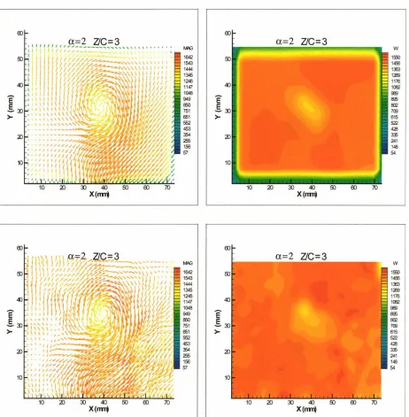
1

Examples of instantaneous and average velocity fields at a streamwise location of 1 chord length behind the wing are presented in Figure 4.8 and Figure 4.9.

The in-plane velocity fields for a= 2° case at this station (Figure 4.8) resemble that taken at ZJC

=

0. Here, the size of the wing tip vortex has clearly increased to a larger size. The wake of the wing is still visible in the a= 2° case. This is a strong indication that the rollup process has not been completed. At a higher angle of attack (Figure 4.9, for a= 10~, the in-plane vector fields in the vortex region look qualitatively

the same as in the lower

a

case. However, in this case, the wake of the wing is no longer noticeable.

(49)

contour for a= 2° case. In the former cases, the out-of-plane velocity fields have lower

magnitude in the regions that resemble an ellipse. However, the corresponding in-plane

vector fields for such cases do not give any indication that the tip vortex is of an elliptical

shape.

4.4.3 Z/C

=

2

The velocity fields for the

a

=

2° case, at a streamwise station of 2-chord length

behind the wing, are shown in Figure 4.1 0. The out-of-plane velocity contours for the

a

=

2° case are now qualitatively similar to the higher angle of attack case (looks like an

ellipse). Also, the out-of-plane velocities in the region near the vortex for all a is now

closer to the freestream velocity compared to that presented in the previous sub-section.

The in-plane and out-of-plane velocity fields for a= 10° case are shown in Figure

4.11. At this downstream station, the in-plane vector plots and out-of-plane contour plots

for a= 10° case are qualitatively the same as those for the corresponding a= I 0° case, at

Z/C

=

1.

4.4.4 Z/C

=

3

Typical average and instantaneous velocity fields measured at a streamwise

station of 3-chord length behind the wing for the low and high angle of attack cases are

shown in Figure 4.12 to Figure 4.13, respectively. These plots are arranged as in

previous sub-sections. The plots, presented here, are qualitatively the same as in Z/C

=

2

(50)

3-Component Velocity Fields Behind the Wing

37

4.4.5 Z/C

=

4

Instantaneous and average velocity fields, for a= 2° and 10° case at streamwise

location of 4-chord length behind the wing, are presented in Figure 4.14 and Figure 4.15,

respectively. Again, with the exception of the magnitude of the velocity components and

the size of the vortex core, there seems to be no qualitative difference between this case

and the case considered in Section 4.4.3.

4.4.6 Z/C

=

5

The streamwise station of 5-chord length behind the model is the final streamwise

station at which measurements are made. Examples of velocity fields obtained from

measurements at this station are shown in Figure 4.16 and Figure 4.17, with the usual

arrangement.

The in-plane velocity vector field for the a= 2° (Figure 4.16) at this station still

resembles that taken at earlier stations. The wake of the wing is still visible, within the

field of view, although it is much shorter than before. (But the tip vortex also has moved

downward, at this station, with respect to the field of view.) The in-plane velocity fields

for a higher angle of attack (a= 1 0~ case still resemble the vector fields presented

previously (see Figure 4.17).

At this downstream station, the shape of the out-of-plane velocity contour in the

(51)

(a=

i).

On the other hand, the shape of the low velocity contour, in the vicinity of the

(52)

3-Component Velocity Fields Behind the Wing

39

Figure 4.1. Schematic of the setup and the coordinate system

Running Averages

200

150 .-.

..!!! ₁₀₀

E • u_avg

.§. ₅₀ • v_avg

Q) _..._{u'_rms}

:I

iii 0 x v' rms

>

-50 50 100 150 200 2 0

-100

Number of fields

(53)

a= 8°, ZJC = 4

X(mm)

a= 8°, ZJC

=

4

1600

1500

-;- 1400

l1300

;: ₁₂₀₀

1100

1000

0 20 40 60

X(mm)

a.

=

8°, ZJC

=

4

10

-40 60

-.Je

:!:.. _-90

~

·c::; -140

:e

₀

> -190

-240

X (mm)

(54)

3-Component Velocity Fields Behind the Wing

41

(55)

a=O ZJC=O

00

a=O ZJC=O

_,, , _ # , . . - - , ,

---- --

.,

ro

,_----

.. ,,

40

e

.§.:ll >-a> 10 MIG 1642 1543 1444 1345 1246 1147 1048 949 BOO 751 ffi1 55:2 453 ~ 2i6 1$ 5/ MIG 1642 1543 1444 1345 1246 1147 1048 949 BOO 751 ffi1 55:2 453 ~ 2i6 1$ 5/

e

.§.

>-e

.§.

>-a=O ZJC=O

X(nm)

a=O ZJC=O

[image:55.540.33.496.114.585.2]

X(nm)

Figure 4.5. Velocity fields, z/c = 0, a= 0° (upper: average, lower: instantaneous)

(56)

3-Component

Velocity

Fields Behind the

Wing

a.=2

ZJC=O

a.=2

ZJC=O

M'G 1642 1543 1444 1345 12<16

«l ₁₁₄₇ «l

1048

e

,.,.

_____

949

e

S:n ...

_

850 751 S:n

> 1:61 >

552 453

2) 354

255 156 57

X(lll'l1 X(lll'l1

ED

,,,_

a.=2

ZJC=O

/ / / , M'G

ro /.., ///.,-_...

__

₁₆₄₂

1543 1444 1345

«l

,

...

-

12«> 1147

e

949 1048

e

S :n 850 751 S:n

> 1:61 >

552

453

354 2)

255

156 57

10

X(lll'l1

Figure 4.6. Velocity fields, z/c = 0, a= 2° (upper: average, lower: instantaneous)

(57)

MOG w

1642 1$)

1543 1<6)

1444 1:El

1:3<6 1a'll

1246 1175

1147 1!112

1048 9tB

e

949

e

!H;

.§. e50 _.§. !(12

751 703

> 651 _> 615

552 522

453 4<13

354 3lj

2S6 241

156 148

fi/ 54

X(rtrri X(rtrri

MOG w

1642 1550

1543 14al

1444 1:El

1345 1a'll

1246 1175

1147 1!112

1048 9tB

949 !H;

e50 !(12

751 703

651 615

552 522

453 4<13

354 3lj

2S6 241

156 148

fi/ 54

X(rtrri

(58)

3-Component Velocity Fields Behind the Wing

00 aJ 10 M'G 1642 1543 1444 1345 1246 1147 1048 949 !5) 751 651 552 453 :fi4 256 156 57 M'G 1642 1543 1444 1345 1246 1147 1048 949 !5) 751 651 552 453 :fi4 256 156 57 40 10

10 20 :ll 40 ro

X(rrn-.

Figure 4.8. Velocity fields, z/c = 1, a= 2° (upper: average, lower: instantaneous)

(59)

M'G w

16<12 ₅₀ 1500

1543 1453

1444 1333

1345 1:a'B

1246

40 1176

1147 1002

1048 SEll

e

949

e

ees

.§. ffiO 751 _.s _~ 002 703

> 651 _> 615

552 522

453 4:B

354 _aJ 3:!i

255 241

156 148

57 54

10

10 aJ ~ 40 50 ro 70

X(llll't X(~

M'G w

1642 1500

1543 1455

1444 1333

1345 1:a'B

40 1246 1147 1176 1002

e

1048 SEll

949

e

ees

.s~ ffiO _.§. 002

751 703

> 651 _> 615

552 522

453 4al

354 3:!i

255 241

156 148

57 54

(60)

3-Component

Velocity

Fields Behind the Wing

47

00

a=2 ZJC=2

M'G w

1642 1~

1543 14ffi

1444 1333

1346 1<Hl

1246

40 1176

1147 1002

1048 !81

949

e

ee;

850

..s~ 002

751 700

661 _> 615

552 522

453 42l

354 _2l 3:!i

256 241

156 146

57 54

10

10 2l ~ 40 00 00 70

X(111'11 X(l11'11

00

M'G w

1642 1~

1543 14$

1444 1333

1345 1<Hl

1246 1176

1147 1002

1048 !81

949 ee;

850 002

751 700

661 615

552 522

453 4al

354 3:!i

256 241

156 146

57 54

(61)

MOG w

1642 1ffi()

1543 1456

1444 1333

1345 1a9

<Kl 1246 ₁₁₄₇ <Kl 1176 1002

e

10<18

e

9ll

949 8ili

S:n 850 751 S:n 002 700

> 661 > 615

562 522

453 4:B

354 _aJ :n;

255 241

156 148

57 54

10

10 aJ 3J <Kl ro 00 70

X(rm1 X(llnl

MOG w

1642 1ffi0

1543 1456

1444 1333

1345 1a9

<Kl 1248 1147 1176 1002

e

10<18 9ll

949

e

8ili

S:n 850 .§. 002

751 700

> 661 _> 615

562 522

453 4al

aJ 354 :n;

255 241

156 148

57 54

10

(62)

3-Component

Velocity

49

ED

a=2 ZJC=3

MOG w

1642 1560

1543 1456

1444 1333

1345 1:<£9

1246 1176

1147 40 1002

1048 !HI

e

949

e

fg;

.5.

850

.5.:~:~ 002

751 700

>- &>1 _>- 615

552 522

453 4al

354 _aJ :n;

255 241

156 146

57 54

10

10 aJ ~ 40 00 ED 70

X(nrrt X(nrrt

ED

MOG w

1642 1560

1543 1456

1444 1333

1345 1:<£9

1246 1176

1147 1002

1048 !HI

949

e

fg;

850

.5.

002

751 700

&>1 _>- 615

552 522

453 4al

354 :n;

255 241

156 146

[image:62.540.36.498.183.654.2]

57 54

(63)

M'G w

1642 151i0

1543 14$

1444 1:El

1346 1:<!!3

1246

40 1116

1147 1(82

10<18 983

949 'E 1m

860

.§.~ 002

751 700

ffi1 > 615

552 522

453 4<B

354 ₂₀ 3:1;

256 241

156 148

57 54

10

10 20 ~ 40 00 00 70

X(ITil'i X(ITil'i

00

M'G w

1642 151i0

1543 14$

1444 1:El

1346 1:<!!3

1246 1116

1147 1<82

10<18 983

949 1m

860 002

751 700

ffi1 615

552 522

453 4<B

354 3:1;

256 241

156 148

57 54

X(ITil'i

(64)

3-Component

Velocity

51

a=2 ZJC=4

M'G w

1642 1500

1543 14ffi

1444 1:El

1345 1239

1246

40 1176

1147 1(132

e