guide prioritization of management actions
CHERYLA. LOHR,1, JIMHONE,2MICHAELBODE,3CHRISTOPHERR. DICKMAN,4AMELIAWENGER,3ANDROBERTL. PRESSEY3
1
Department of Parks and Wildlife, Science and Conservation Division, 37 Wildlife Pl, Woodvale, Western Australia 6026 Australia 2
Institute for Applied Ecology, University of Canberra, Canberra, Australian Capital Territory 2601 Australia 3
Australian Research Council Centre of Excellence for Coral Reef Studies, James Cook University, Townsville, Queensland 4811 Australia 4
School of Life and Environmental Sciences, University of Sydney, Sydney, New South Wales 2006 Australia
Citation:Lohr, C. A., J. Hone, M. Bode, C. R. Dickman, A. Wenger, and R. L. Pressey. 2017. Modeling dynamics of native and invasive species to guide prioritization of management actions. Ecosphere 8(5):e01822. 10.1002/ecs2.1822
Abstract. Action to achieve biodiversity conservation is usually expensive, and resources are limited rel-ative to conservation goals. Prioritizing management investment therefore is essential if important goals are to be achieved. New software, the“Islands DSS,”has been developed to prioritize the mix of manage-ment actions that will optimally mitigate biodiversity loss. Here, we present novel temporally dynamic models of species population growth, interaction, and management efficacy that have been incorporated into the software. We have analyzed the sensitivity of these models to uncertainty in four parameters: max-imum rate of population growth (rmax), coefficient of species interaction (aij), quantity of food resources required to maintain species equilibrium (Ji), and the coefficient of management efficacy (hi). We focused on the projected abundance of species by simulating interactions among one to four species, both invasive and native, on a hypothetical arid-tropical island that is 1000 ha in size and consists offive evenly dis-tributed habitat types. Sensitivity analysis revealed significant variation in species abundance due to uncer-tainty in rmax (coefficient=51.34;P<0.001) and aij (Ni=16.48; P=0.43; Nj=2.332; P=2.0016), a significant but potentially stabilizing effect of modeling multiple species simultaneously (coeffi -cient=65.80;P=2.0016), and mirroring by species response trajectories of threat mitigation trajectories. There are several benefits of using temporally dynamic models of species responses to threat mitigation in systematic conservation planning including increased accuracy in estimates of the cost of management; locally relevant understanding of lag-times between threat establishment and unacceptable impacts on val-ued species; understanding of threat abundance and required intensity of control for biodiversity features to persist; site- and species-specific understanding of time to eradication and threat recovery when man-agement is interrupted; and an improved understanding of the opportunity cost, in terms of threat levels and responses of native species, for islands not selected for management. Our models and associated soft-ware are based on decades of ecological research, potentially useful in a wide range of situations, including islands, the mainland, and marine regions, and we suggest that they provide managers with novel and powerful tools to efficiently prioritize conservation actions via the new systematic conservation planning software,“Islands DSS.”
Key words: conservation planning; invasive species; sensitivity analysis; species response trajectory; threat mitigation.
Received8 December 2016; revised 30 March 2017; accepted 3 April 2017. Corresponding Editor: Lucas N. Joppa.
Copyright:©2017 Lohr et al. This is an open access article under the terms of the Creative Commons Attribution License, which permits use, distribution and reproduction in any medium, provided the original work is properly cited.
INTRODUCTION
Invasive species are one of the primary threats to the persistence and conservation of native spe-cies (Butchart et al. 2010, Ehrenfeld 2010, Duncan et al. 2013). These species can be controlled or eradicated (Veitch and Clout 2002), but effective control is usually costly and resource intensive and may compete with other threats such as per-secution by people or loss of habitat as priorities for mitigation. Prioritization of threat manage-ment is therefore essential because human and material resources are limited relative to the cost of achieving many conservation goals.
While conservation goals are best pursued using a range of management actions, most pri-oritization research has focused on the design of networks of conservation reserves rather than considering the mix of management actions that will optimally mitigate biodiversity loss (Pressey et al. 2004, Wilson et al. 2007, Spring et al. 2010, Visconti et al. 2010). Previous prioritization exer-cises that have considered a range of possible actions (Bottrill et al. 2008, Joseph et al. 2008) have either modeled the effect of management on a threat and the responses of protected species to threat mitigation separately, or assumed that threats are static and eliminated instantaneously (or uniformly over time) when conservation actions are applied (Watts et al. 2009, Klein et al. 2010, Wilson et al. 2010, Januchowski-Hartley et al. 2011).
New systematic conservation planning software, the“Islands DSS,”has been developed to prioritize the mix of management actions that will optimally mitigate biodiversity loss. The optimization algo-rithm within the software is designed to use con-tinuous ecosystem or community models with temporally variable trajectories of species abun-dance, henceforth referred to as“species response trajectories” (Brotankova et al. 2015, Urli et al. 2016). The shape of a species response trajectory may be influenced by the presence of other inter-acting species or threat mitigation activities. Incor-porating continuous species response trajectories into systematic conservation planning models can improve the accuracy of estimates of the cost of management by up to 20% (Cattarino et al. 2016). Ultimately, the software uses a constraint program-ming model built upon robust optimization princi-ples and a large neighborhood search scheme to
select a suite of management actions that will max-imize the total conservation benefit achieved given a limited budget (Urli et al. 2016). It can also help to identify the most cost-effective management actions to implement (Margules and Pressey 2000). Here, we present the novel temporally dynamic and spatially implicit ecological community mod-els with dynamics that are directly and indirectly influenced by management actions that have been embedded in the new software.
Modeling the effects of invasive species on pro-tected native species can be complex and, to be effective, needs to be underpinned by sound eco-logical understanding. This is because, when invasive species become established in ecological communities, they often become involved in webs of direct and indirect interactions with other spe-cies that can generate surprising relationships (Dickman 2007). For example, on Boullanger Island, Western Australia, the removal of invasive mice (Mus musculus) led to a short-term depres-sion in numbers of a threatened native marsupial (the dibbler, Parantechinus apicalis) and concomi-tant increases in litter-dwelling skinks (Ctenotus
fallens andMorethia lineoocellata) (Dickman 2007).
Unexpected interactions may also occur due to hyperpredation or mesopredator release, exempli-fied by rabbits killing birds (Courchamp et al. 2000) and coyotes protecting birds by reducing other predators (Crooks and Soule 1999), or to synergistic interactions between invasive species and other threats (Doherty et al. 2015).
Users of the “Islands DSS” software need a sound understanding of the ecological commu-nity model and associated assumptions embed-ded within the code to assess the quality of the recommendations generated by the optimization algorithm. Therefore, we present the compo-nents of the ecological community model and discuss the data input requirements. We also present the results of sensitivity analysis of uncertainty in four model components: maxi-mum intrinsic rate of population growth (rmax), coefficient of species interaction (aij), quantity of
food resources required to maintain species equi-librium (Ji), and the coefficient of management
effectiveness (hi), by simulating interactions
among one to four species on a hypothetical 1000-ha island.
Inputs for the sensitivity analysis are based on species found on the Pilbara Islands, Western Australia, a hotspot for endemic species that has recently been the focus of intense conservation research. The software and our sensitivity analy-sis use islands as a case study because the num-bers of species present on islands are limited, thus reducing computational demands, and because islands often contain endemic species as well as invasive species that threaten native spe-cies via competition or predation (e.g., Dickman 1992). The modeling approach could, however,
be used for mainland and marine applications. The ecological community models and the asso-ciated software synthesize decades of ecological research to provide conservation practitioners with estimates of site- and species-specific com-munity dynamics.
METHODS
Modeling population dynamics for conservation
planning software
Broadly, the ecological community models are built upon theories of bioenergetics (Ney 1993) and resource availability (McLeod 1997). Many species are limited primarily by food availability and secondarily by density-dependent factors that intensify as carrying capacity is approached. To reduce the data input requirements for the software, we assumed that populations within the community are closed, existing on islands with limited external resources. We usefinite dif-ference equations to describe temporal changes in abundance of speciesi, using a one-year time step. For all species, in the absence of competi-tors, consumers, and management, a population of species i will show logistic growth. Concur-rently, we assume management inputs (Aa) have
[image:3.612.84.530.482.689.2]diminishing returns (Hone et al. 2015). Model parameters are defined in Table 1.
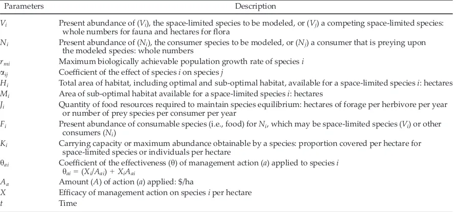
Table 1. Description of parameters within the two models (Eqs. 1 and 2) of population dynamics for island species.
Parameters Description
Vi Present abundance of (Vi), the space-limited species to be modeled, or (Vj) a competing space-limited species: whole numbers for fauna and hectares forflora
Ni Present abundance of (Ni), the consumer species to be modeled, or (Nj) a consumer that is preying upon the modeled species: whole numbers
rmi Maximum biologically achievable population growth rate of speciesi aij Coefficient of the effect of speciesion speciesj
Hi Total area of habitat, including optimal and sub-optimal habitat, available for a space-limited speciesi: hectares Mi Area of sub-optimal habitat available for a space-limited speciesi: hectares
Ji Quantity of food resources required to maintain species equilibrium: hectares of forage per herbivore per year or number of prey species per consumer per year
Fi Present abundance of consumable species (i.e., food) forNi, which may be space-limited species (Vi) or other consumers (Ni)
Ki Carrying capacity or maximum abundance obtainable by a species: proportion covered per hectare for space-limited species or individuals per hectare
hai Coefficient of the effectiveness (h) of management action (a) applied to speciesi hai=(Xi/Aai)+XiAai
Aa Amount (A) of action (a) applied: $/ha
X Efficacy of management action on speciesiper hectare
The ecological community models consist of two equations. The first describes the dynamics of space-limited species under competition from other space-limited species (Eq. 1), which are defined as either primary producers or species that consume resources from outside a given island’s environment (e.g., marine turtles, sea-birds). The abundance of these latter species is limited by the area of suitable habitat for non-consumptive purposes (e.g., nest sites). Access to this habitat and reproductive success may be suppressed by competition with other species.
Two space-limited species (Vi and Vj) with
competition (competitive coexistence or competi-tive exclusion) is shown in below
Viðtþ1Þ
¼Vi;tþrmiVi;t 1
Vi;tþPj2BiaijVj;t
KiHiKiMi
P
j2CiaijVj;t 1þPj2
CiaijVj;t
0 B B B @ 1 C C C A X
j2Di
aijVi;tNj;t
X
a
Vi;t haiAaðtÞ 1þhaiAaðtÞ
(1) Two outcomes of interspecific competition are included within Eq. 1: competitive coexistence and exclusion. The form of competition (resource or interference) is not defined to accommodate a wide variety of potential species interactions, but we assume linear effects of competition (Table 3) to reduce data input requirements. If two species can coexist despite interspecific competition (Bengtsson et al. 1994), they may occupy the same habitat type simultaneously but the carry-ing capacity for each species is suppressed by the coefficient of the species interaction (Table 1:aij).
The identity of a species that competes with (but does not exclude) speciesi is contained in setBi
(Eq. 1: j 2Bi). Under competitive exclusion, by
contrast, two competing species may not coexist within a given habitat type and instead will retreat from any sub-optimal habitat types to their respective optimal habitat types where they retain competitive dominance. The identity of species that exclude species iis contained in set
Ci(Eq. 1:j 2Ci).
The second equation describes the dynamics of consumers whose resources are contained within the boundary of a given island (Eq. 2). The
abundance of a consumer is limited primarily by the amount of energy it requires to reproduce (Ji)
and the abundance of its food resources (Ni/ΣFi)
(Table 1), and secondarily by other density-dependent factors (Ki), such as space. It is
assumed in Eq. 1 that consumers have a linear (type 1) functional response (Holling 1965). The numerical response of consumers to their food includes a ratio term. Empirical evidence for such a ratio response has been reported for wolves (Canis lupus) eating moose (Alces alces) in North America (Eberhardt and Petersen 1999), ferrets (Mustela furo) eating rabbits (Oryctolagus
cuniculus) in New Zealand (Barlow and Norbury
2001), least weasels (Mustela nivalis) eating voles
(Microtus agrestis) in Scandinavia (Hanski et al.
2001), and lynx (Lepus canadensis) eating snow-shoe hare (Lepus americanus) in Canada (Hone et al. 2007).
Consumers (Ni) that consume food (Fi) and
may in turn be consumed (Nj) is shown in below
Niðtþ1Þ
¼Ni;tþrmiNi;t 1Ji
Ni;t
RFi
1Ni;t
Ki
X
j2Di
aijNi;tNj;t
X
a
Ni;t haiAaðtÞ
1þhaiAaðtÞ
ð2Þ
Parameterizing the models
A limitation of some models is that their input requirements can appear to be complex or daunt-ing. Here, we describe the ideal sources of data that should be used in our models, and also indicate alternative data sources that are more likely to be available in real-world situations (Table 2) such as those available for islands in the Pilbara.
Present abundance of a species (
N
ior
V
i)
temporally or geographically limited survey data and species attributes (Potts and Elith 2006), eli-cited from experts (Anadon et al. 2009, Martin et al. 2012), or replaced with presence-only data (Table 2). The use of presence-only data requires some assumptions: (1) For pest species that have
been present for a long time or for native unthreatened species, we assume species abun-dance is at carrying capacity (Ki); (2) for newly
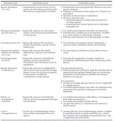
[image:5.612.81.534.94.576.2]arrived pest species, we assume that current abundance is at or just above the minimum propagule size for population establishment Table 2. Ideal and actual sources of data on population parameters for island species.
Parameter type Ideal data source Actual data source
Species abundance (ViorNi)
Comprehensive recent census of each species on each island, quantifying the fluctuations in populations over time
•
Extrapolation from geographically limited surveys and species attributes•
Estimates of abundance from experts for all species on each island•
Sporadic or old measures of abundance•
Presence-only data and:◦
assuming long-term resident species present at carrying capacity◦
assuming newly arrived species are at minimum propagule sizeMaximum population growth rate (rmi)
Empirically measure on each island using a small and growing population of each species
•
Usefield-based estimates from other environments•
Estimate from complete set of demographic variables (e.g., Leslie matrix or Lotka-Euler equation)•
Estimate using minimal set of demographic variablesCarrying capacity (Ki) Empirically measure the maximum density obtained by a species in each habitat type
•
Use estimates of maximum density obtained by a species in other, preferably similar environmentsOptimal/sub-optimal habitat classification (HiorMi)
Empirically measure the density obtained by a species in each habitat type
•
Use descriptions of habitat use from other environ-mentsFood requirement (JiandFi)
Empirically measure in thefield the quantity of food consumed by individuals when the species exists in equilibrium
•
Calculate the megajoules of energy required or provided by individuals given the average mass of the speciesSpecies interaction coefficient (aij)
Empirically measure in multiplefield sites to derive species-specific damage– density curves for each pair of species, in the presence of different
combinations of other species
For space-limited species:
•
Estimate pairwise coefficients using the identification of optimal and sub-optimal habitat types to calculate the proportion of total habitat availability that must be shared by two speciesFor consumers:
•
Assume an existing damage–density curve is applicable to multiple species•
Usefield-based estimates from other environments and assume that the quantity of damage is not density dependentEfficacy of management action (hi)
Empirically measure in thefield the efficacy of each management technique on each threat
•
Usefield-based estimates of the efficacy of management from other environments•
Use expert knowledge to define efficacy•
Assume that efficacy is consistent across related or similar speciesCost of
management (Aa)
Use the cost of implementing actions from similar environments for each species
•
Assume that the cost of implementing actions is related to quantified island or species attributes (e.g., island size, distance from mainland, transportation costs, rate of application per individual)(Forsyth and Duncan 2001); and (3) for native spe-cies that have been in the presence of a threat for a moderate to long period of time, we assume that their abundance has been suppressed to half of carrying capacity (Ki/2).
Intrinsic rate of population growth (
r
mi)
The instantaneous rate of population growth (rmi) is a critical parameter for modeling changes
in abundance in species over time. Actual rate of population growth may vary greatly across the landscape, with optimal habitats allowing popu-lations to grow more rapidly than sub-optimal habitats (Pulliam and Danielson 1991). Species in equilibrium should have a realized growth rate of approximately zero as the population fluctu-ates around carrying capacity. The maximum annual population growth rate, rmax, is the increase in numbers that occurs when resources are not limiting and there are no predators, para-sites, or competitors (Sibly and Hone 2002). Our models calculate the realized growth rate by combining rmax with data on the number of predators, competitors, or resources available on a given island at a given time.
In an ideal situation, values ofrmax would be estimated empirically for each species of interest on each island (Table 2). Unsurprisingly,rmaxhas not been estimated in thefield for the vast major-ity of species (Duncan et al. 2007), typically because long-term field studies are logistically
and financially difficult. However, rmax may be
estimated from minimal demographic data, namely age at first reproduction, given demo-graphic data on related species (Hone et al. 2010). While there is considerable uncertainty around predicted values ofrmax, they confer the advantage of consistent assumptions and level of uncertainty across species and islands when used in conservation planning software.
Estimating rmax for plants is less reliable. Plants have a wider variety of reproductive strategies and may produce hundreds or thou-sands of diaspores per parent per year. However, many of these will never contribute to the next generation. Where possible, estimates of rmax should be derived fromfield studies of small but rapidly growing plant populations (Gimeno and Vila 2002). Alternatively, knowledge of a plant’s reproductive strategy and a patch expansion rate (Dixon et al. 2002), or relative growth rate
(Traveset et al. 2008), could be used to calculate a rate of population growth.
Carrying capacity (
K
i)
Carrying capacity generally refers to the maxi-mum sustainable number of individuals that can be achieved in a given habitat (McLeod 1997). Quantifying carrying capacity is necessary for defining the upper bounds on species abundance and subsequently for modeling increases and decreases in interacting species. It is a particularly pertinent variable for species that are naturally rare vs. those that are rare due to threatening processes (Partel et al. 2005) because conservation actions are unlikely to generate the desired outcome if a spe-cies is subject to natural causes of rarity.
Where ideal data are not available (Table 2), carrying capacity for space-limited species may be based on the maximum density a species has achieved in similar environments multiplied by the amount of suitable habitat present. In the equations above, the increase in consumers (Eq. 2) is limited by two carrying capacity terms. First, carrying capacity is defined by food avail-ability (seeFood required(Jiand Fi)) as the point at
which resource consumption by a species is equal to population growth rates of its prey (McLeod 1997). Second, in the event that food resources are exceedingly abundant, consumer population growth may be limited by other density-depen-dent factors (Ki; e.g., shelter, space, water).
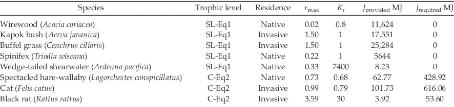
Separating food from other density-dependent factors is particularly relevant in tropical arid environments where food resources may be spo-radically abundant and interspersed with harsh, dry periods. For example, the carrying capacity for black rats (Rattus rattus) in dry forests and grassland is approximately 30 rats/ha, whereas the maximum observed on wet tropical islands is 119 rats/ha (Harper and Bunbury 2015). Two terms for carrying capacity are useful when pri-oritizing conservation actions because it allows the effective carrying capacity (food requirement) to differ among islands despite a consistent coef-ficient of carrying capacity for each species.
theory is the idea that organisms will enlarge an activity as long as the resulting gain in time spent per unit food exceeds the loss (MacArthur and Pianka 1966). The most productive habitat types will be optimal until density-dependent factors reduce the amount of resources available per indi-vidual within patches of that habitat, at which point individuals will disperse into other, less optimal habitat patches. Current application of this theory is frequently seen in habitat suitability models where regressions link species occupancy data with landscape-scale habitat maps and iden-tify sub-optimal and optimal habitat types (e.g., Carvalho and Gomes 2003) or patches of high spe-cies density (Guthlin et al. 2014).
The continuum of variable habitats across a landscape will usually have to be grouped into a limited number of classes (Table 2). Depending on the available literature, allocation of optimal or sub-optimal habitat types to each species should then be biased toward sub-optimal habi-tats to limit the invasive potential of generalist species within the models (e.g., Appendix S1: Table S1).
Food required (
J
iand
F
i)
The primary limit to population growth is built on bioenergetics theory (Ney 1993) and relies on Ji, the estimated amount of food per
head of species irequired to maintain a popula-tion at equilibrium. Unfortunately, many bioen-ergetics models require large quantities of species-specific data to calculate multiple param-eters, and hence have potential for inaccuracy (Ney 1993). Encouraging land managers to use a systematic conservation planning tool requires that we minimize data requirements. We used estimates of species basal metabolic rate (BMR) to derive the amount of food required by each species. Despite debate regarding modeling tech-niques and variation among species (see Roberts et al. 2010, Seymour and White 2011), current models for BMR in animals weighing less than 2.5 kg do not deviate dramatically from Brody’s equation (Eq. 3), in which daily BMR is mea-sured in megajoules MJ andWis weight in kilo-grams (Brody 1945). Given advances in island conservation and eradication, it is now rare that managers would be required to prioritize the management of invasive species that are consid-erably larger than 2.5 kg (Clout and Veitch 2002).
BMRðMJÞ ¼ 0:27W0:75 (3)
Basal metabolic rate alone will underestimate the energy requirements of wild animals, because foraging, movement, and reproduction consume energy. Efficiency of digestion and metabolism varies, with efficiencies of 70–80% being typical (Case 1973, McDonald et al. 2002). To account for the energy requirements of forag-ing and reproduction in the wild, we multiplied BMR by 150%. Similarly, to account for metabolic efficiency, we divided BMR by 75% for carni-vores and omnicarni-vores and by 50% for herbicarni-vores to estimate the total amount of energy an animal needs to survive (Eq. 4).
Annual consumptionðMJÞ
¼ 365 1:5 0:27W 0:75 0:75
or
365 1:5 0:27W 0:75 0:50
(4)
The gross energy (GE) content of prey items depends on the proportions of carbohydrates, fats, and proteins within the food (McDonald et al. 2002). In lieu of measuring the chemical energy present in all prey items within an ecosystem (Table 2), we used average GE con-tent per weight (Wi) of animal prey and
vegeta-tion class. Since vegetavegeta-tion abundance is measured in hectares, the GE content of vegeta-tion must be multiplied by biomass of each plant species as if it achieved complete coverage of a hectare. If relevant biomass functions are unavailable, biomass functions for similar spe-cies may be used. For example, in lieu of bio-mass functions for tropical arid zone plants on the Pilbara Islands (Table 4), we used a foliage biomass function for sagebrush (Artemesia
tri-dentate; Gholz et al. 1979), which grows in arid
and semi-arid conditions of northwest America. The total number of prey items or hectares of vegetation required by a predator is a function of prey size or vegetation biomass and energy requirements of the consumer (Eq. 5).
JiðNumber of prey required annuallyÞ
¼
365 1:5 0:27W 0:75
j 0:75
!
GE Wi
Species interactions (
a
ij)
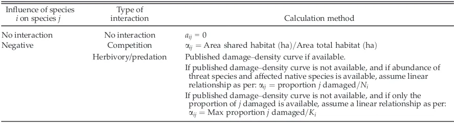
The coefficient of species interaction is based upon the concept of a damage–density curve, which is a linear or curved relationship between the amount of damage done by a pest and the abundance of the pest (Hone 2007). Within the systematic conservation planning software, a coef-ficient must be defined for every pair of interact-ing organisms. For space-limited species, the coefficient is calculated as the proportion of habi-tat that two species share (Eq. 1; Table 3). For con-sumers, the coefficient is derived from the proportion of a population of a prey species taken by each individual predator per annum (Table 3).
Due to the number and complexity of species interactions that may occur in a community (Polis and Strong 1996), estimates of species interaction coefficients are made pairwise. They hence assume a linear functional response (Hol-ling 1965) and that interaction coefficients may be conveyed among similar species (Table 3; Appendix S1: Table S2). We assumed that all rela-tionships have an intercept of zero and that there is no variation in predator search effort or cap-ture success across similar prey items. For exam-ple, given similarities in size, habitat use, and reproductive strategy, the herbivorous marsupial
Lagorchestes conspicillatuswould be similarly
sus-ceptible to predation by feral cats (Felis catus) as
Bettongia penicillata(Dickman 1996). Similarly, we
assume that rooting of soil by pigs (Hone 2007) will have an equivalent negative influence on all plant species that are not disturbance specialists.
Efficacy of management actions (
h
aiand
A
a)
The purpose of these equations is to create a temporally dynamic model of island species
abundance that may be modified directly or indi-rectly by management actions. The term for man-agement efficacy describes the portion of a threat population that is removed by a given manage-ment action. The estimated efficacy of an action may vary depending on the measurement tech-nique, management site, time of year, and the extent and magnitude of application (Table 1), but may be derived from the literature (e.g., Wil-liams and Moore 1995, Johnston et al. 2010, Van-derWerf et al. 2011, Coddou et al. 2014) or from expert knowledge of how the techniques have worked in different environments (Table 2).
Sensitivity analysis of model components
The above equations were recreated in RStudio (2015) using R version 3.2.5 for a hypothetical island of 1000 ha that contains five evenly dis-tributed habitat types and a community of one to four interacting species, both native and invasive (Table 4; Appendix S1: Tables S1, S2). Both the habitat types and species were chosen to repre-sent those that occur in the Pilbara case study region, with the native and invasive species among those that are most commonly targeted by managers for conservation and control, respectively. The modeling time frame was lim-ited to 20 yr; few management agencies are likely to forecast species declines or recoveries more than 20 yr in advance.
The sensitivity of model results to variation in four key components (rmax, aij, Ji, and hai) was
assessed by independently randomizing the input value of each component over 100 simula-tions. We varied the values for rmax, aij, and Ji
[image:8.612.84.528.97.218.2]using a normal distribution (mean, Table 4). We used a uniform distribution between 0 and 1 to Table 3. Actual methods of calculating species interaction coefficients.
Influence of species ion speciesj
Type of
interaction Calculation method
No interaction No interaction aij=0
Negative Competition aij¼Area shared habitatðhaÞ=Area total habitatðhaÞ Herbivory/predation Published damage–density curve if available.
If published damage–density curve is not available, and if abundance of threat species and affected native species is available, assume linear relationship as per:aij¼proportionjdamaged=Ni
vary the values for hai. We then analyzed the
variation in species abundance in year 20 in rela-tion to variarela-tion in the model component using linear regression models with fixed and random effects (Pinheiro et al. 2017). Data were not trans-formed prior to analysis. With combinations of one to four species, two models for competition, and 100 simulations, up to 16,000 results for year-20 abundance were analyzed. The input val-ues in Table 4 and Appendix S1: Tables S1, S2 were derived from an extensive literature review (C. Lohr,unpublished data).
R
ESULTSSensitivity analysis of species population growth
rate
r
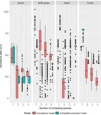
maxAs would be expected, variation in the input value of rmax significantly affects the 20-yr abun-dance of species (coefficient= 51.34; P< 0.001; Appendix S1: Table S3). Increasing the number of species included in the modeled ecosystem signifi-cantly reduces the median and variation in 20-yr abundance of the modeled species due to compe-tition for resources (P< 1.005; Fig. 1; App-endix S1: Table S3). Similarly, within a given number of species, the choice between defining a competitive exclusion relationship or a competitive coexistence relationship between two space-lim-ited species makes a difference in the average abundance of species i in year 20 (P< 1.005, Fig. 1; Appendix S1: Table S3). The influence of the variation inrmaxis more constrained in species interactions that involve competitive exclusion because species are pushed out of sub-optimal habitats and effectively confined to optimal habitat
types, or parts thereof, whereas competitive coex-istence allows two or more species to occupy the same habitat type. With fewer habitats to effec-tively occupy under competitive exclusion, there is less room for variation in species abundance. A mixed-effects model with rmax, competition type, and number of species included as variables explains 79% of the variation in the data (Appendix S1: Table S3).
Sensitivity analysis of species interaction
coefficients
a
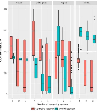
ijVariation in the species interaction coefficient does not have a significant influence on the varia-tion in the year-20 abundance for modeled species
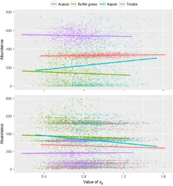
iwhen it is involved in a competitive relationship (paij = 0.43; competitive coexistence linear regres-sion for species i; F12, 7764= 1807, P <2.0016, r2= 0.73). The total number of species included in the ecosystem, however, does have a significant indirect effect on the year-20 abundance for mod-eled species i (P= 2.0016, Fig. 2; Appendix S1: Table S4). In contrast, variation in both the species interaction coefficient and the number of species included in the ecosystem has a significant indirect effect on the year-20 abundance of competing species j (paij = 2.0016; pno. of species =2.0016; F12, 15627= 414.3, P <2.2016, r2=0.24, Fig. 3; Appendix S1: Table S5). It is also evident in Fig. 3 that the identity of the species involved in interac-tions also significantly influences the year-20 abundance of species (Appendix S1: Tables S4, S5).
Sensitivity analysis of prey consumed
J
iJi is a component of the food resource-based
[image:9.612.84.527.111.216.2]carrying capacity term in Eq. 2. Increasing Ji
Table 4. Input values for simulations of species trajectories on an island that is 1000 ha in size and hasfive habi-tat types (Appendix S1: Table S1).
Species Trophic level Residence rmax Ki JprovidedMJ JrequiredMJ
Wirewood (Acacia coriacea) SL-Eq1 Native 0.02 0.8 11,624 0 Kapok bush (Aerva javanica) SL-Eq1 Invasive 1.50 1 17,551 0 Buffel grass (Cenchrus ciliaris) SL-Eq1 Invasive 1.50 1 25,284 0 Spinifex (Triodia wiseana) SL-Eq1 Native 0.22 1 5644 0 Wedge-tailed shearwater (Ardenna pacifica) SL-Eq1 Native 0.33 7400 8.23 0 Spectacled hare-wallaby (Lagorchestes conspicillatus) C-Eq2 Native 0.73 0.68 62.77 428.92 Cat (Felis catus) C-Eq2 Invasive 0.99 0.79 101.73 616.06 Black rat (Rattus rattus) C-Eq2 Invasive 3.59 30 3.92 53.60
reduces the margin between current species abundance and the food-based carrying capacity of the ecosystem, alters the magnitude of fluctua-tions around the food-based carrying capacity, and acts as a linear brake on the growth of the modeled species (i) population. Depending on the food resources available on an island,Ji,and
the corresponding Fi (food resources available)
can prevent population growth before species i
reaches its ultimate carrying capacity (Ki).Jihad
an insignificant effect on the abundance of
speciesi(P= 1.00) when compared to the
signifi-cant influence of the number of species (P =8.004) included in the modeled ecosystem and the trophic level of species i (linear mixed-effects model r2= 0.73; Appendix S1: Table S6). The abundance of food items (e.g., plants) is indi-rectly related to the Jiof herbivores (e.g., rats or
wallabies). The abundance of consumers is indi-rectly related to their assigned values of Ji. The
interaction between Ji and the plant or predator
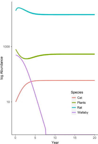
[image:10.612.138.476.83.468.2]different roles in the ecosystem. Plants were pushed to a minimal abundance that maintained the rat population at equilibrium, whereas cats were not food limited and were maintained at maximum density (Kcat) regardless of Ji
(Appendix S1: Table S6). When all four species were included in the ecosystem, wallabies became extinct within 7 yr due to hyperpredation by cats, whereas rats became food limited (20-yr abun-dance~0.5 9Krat), following a reduction in plant resources when two herbivores were present (Fig. 4).
Sensitivity analysis of the effectiveness of
management (
h
i)
[image:11.612.137.475.83.469.2]F1, 298 =2.34; adjr2=0.87) and the year-20 abun-dance of wallabies increased (coefficient= 1164.36; P< 2.0016; Model F1, 298 =69.96; adj r2=0.86; Appendix S1: Table S7). The proportion of cats removed per year explained approximately 87% of the variation in the year-20 abundance of cats and wallabies. Fitting a three-parameter logistic equation to the efficacy of management against the proportional reduction in year-20 cat abundance (r2=0.99), we calculated an inflection
point of 0.40 (95% CI 0.36–0.50), which coincided with the difference between cat populations that stabilized within 20 yr vs. populations that were continuing to decline after 20 yr (Fig. 5). Cat
extinction occurred within 20 yr if hcatwas more than 0.54.
Two carrying capacity terms (K and prey availability) induced compensatory population growth of cats in response to the removal of cats from the population. When these two terms were included as factors in the analysis of the variation in the year-20 abundance of cats, the model adjustedr2value increased to 0.99 (Appendix S1: Table S8). In these modeling scenarios,Kwas the more stringent limiting factor, and hence, prey availability was not a significant explanatory variable for cat abundance (coefficient= 0.02;
[image:12.612.137.477.84.450.2]of the effect of the coefficient of management effi-cacy on the abundance of the protected feature was indirectly determined by the coefficient of species interaction (aij). The year-20 abundance
for species j (i.e., the feature) significantly
decreased as aij increased, meaning when aij is
high an individual predator has greater impact on a population of a feature than whenaijis low.
Therefore, threat mitigation activities will yield greater returns when aijis high than when aijis
low.
DISCUSSION
Conservation goals can be achieved using a variety of management actions, with optimal actions being identified and prioritized most often
for single species (Wilson et al. 2007, Bottrill et al. 2008, Joseph et al. 2008, Januchowski-Hartley et al. 2011). Our equations of community dynam-ics and management extend these approaches using spatially and temporally dynamic threat mitigation and species response trajectories that we incorporate into new systematic conservation planning software. While the use of dynamic spe-cies response trajectories can reduce total budget costs by up to 20% compared with traditional static methods (Cattarino et al. 2016) and hence significantly alter recommended management actions, a prioritization algorithm that could incor-porate dynamic species models is a recent devel-opment (Brotankova et al. 2015, Urli et al. 2016).
Unfortunately, most ecosystems include some poorly studied species that are a priority for management agencies. The input values for these species will necessarily involve uncertainty that may not be reduced in the near future. The novel purpose of our sensitivity analysis was to reveal, in the context of uncertain population parame-ters, the behavior of the threat mitigation and species response trajectories and facilitate under-standing of model components for users of the conservation planning software. Other research has demonstrated that halving the variance on parameters with the largest correlation coeffi-cients produces the greatest refinement to model predictions (Gardner et al. 1981). For many spe-cies, those parameters are going to be the initial species abundance and environmental carrying capacity (Appendix S1: Table S8), given that the influence of all other parameters is constrained by this ceiling.
The three key model behaviors revealed by our sensitivity analysis are significant variation in 20-yr species abundance due to parameter uncertainty, a significant and potentially stabiliz-ing effect of modelstabiliz-ing multiple species simulta-neously (Fig. 1), and response curves of native species mirroring threat mitigation trajectories, albeit with species-specific lag-times (Fig. 5).
Increasing the number of species included in the ecosystem model reduced the influence of uncertainty in the species growth rate (Fig. 2). The number of species included in the ecosystem was also a significant covariate when there was uncertainty in the coefficient of species interaction (aij) or food required to maintain species
[image:13.612.87.295.82.386.2]equilib-rium (Ji), but it influenced the value of species
year-20 abundance rather than variation in abun-dance by altering the amount of resources (i.e., habitat or food) available. While ecosystem stabil-ity can be measured by many metrics, our results are consistent with the consensus view that greater species diversity within an ecosystem increases ecosystem stability in the face of pertur-bations (Ives and Carpenter 2007). Similarly, the construction of food webs with plausible interac-tion strengths (species interacinterac-tion matrix; aij;
Appendix S1: Table S2) also improves stability of the modeled ecosystem (McCann 2000). More importantly, it suggests that the results of the
prioritization process will be less subject to uncer-tainty if multiple species are included.
[image:14.612.139.481.81.454.2]two species (aij) and generates dampening
oscilla-tions around equilibrium levels of predator and prey abundance. Increasing the value of aij
increases the magnitude of the oscillations. Lag-times generated by the latter case provide crucial information for managers to visualize, because the return (i.e., increase in species targeted for conser-vation) on management investment may take years or decades (e.g., protecting marine turtle nests when turtles take 30–50 yr to reach repro-ductive maturity).
The linear (type 1) functional response between predators and prey (Holling 1965) is responsible for the species response trajectories mirroring threat mitigation. As mentioned, the decision-sup-port software that will use these equations may be applied to poorly studied areas with many under-studied species. A linear functional response pro-vides the simplest relationship between predators and prey and hence reduces the effort to define input values. However, when compared with type II or III functional response curves, which are both asymptotic, a linear functional response will over-estimate the effects of an invasive species when prey is at high densities, and potentially underes-timate the number of prey taken when predators are at low density but engage in targeted or sur-plus killing (Zimmerman et al. 2015). Sursur-plus kill-ing has been linked to low prey densities and sporadic food supply (e.g., breeding seabird pop-ulations; Oksanen et al. 1985, Major and Jones 2005), both of which are common occurrences on islands. In a biosecurity context, surplus killing has also been linked to the reinvasion/invasion of an ecosystem by an invasive species that is not currently established (Short et al. 2002). A type III sigmoidal functional response is the more appro-priate curve for describing the impact of predators that engage in prey switching or surplus killing, but would be more complicated to define for les-ser-studied species.
With regard to threat mitigation, one of the most important outputs for managers to be able to access is the extinction threshold, which is also known as the sustainable harvest threshold (Slade et al. 1998, Hone et al. 2010), and the asso-ciated time to extinction. Removing the threshold amount of a population annually will stop popu-lation growth and stabilize species abundance, whereas removing more of a population than is defined by the threshold will eventually drive it
to extinction. The extinction threshold is directly related to a species’ maximum annual rate of population growth (rmax). For cats, with rmax of 0.99 (Table 4), Hone et al. (2010) predicted that the extinction threshold will be 0.57. In our simu-lations, which started with 20 cats, at least one cat was still present after 20 yr if the proportion of cats removed annually was less than or equal to 0.54. If 57% of the population was removed annually, cats were extinct within 15 yr.
Other software has been designed to calculate species interactions for the purposes of managing an environment, including Ecosim/Ecopath (Chris-tensen and Walters 2004). Ecosim/Ecopath uses a similar bioenergetics framework to model species interactions. However, Ecosim/Ecopath, which is designed for use in managed fisheries, requires many variables, including biomass accumulation rate, diet composition, and migration rate, that could not be defined for poorly studied terrestrial ecosystems or species. Our equations have a reduced data requirement through the use of sev-eral assumptions: (1) Islands are closed ecosystems with no net migration; (2) species abundance is limited by the amount of habitat and food avail-able; (3) the quantity of habitat shared by two spe-cies is a suitable proxy for competition, which may occur via many different interactions; and (4) species interact with their habitat, other species, and management, which occurs in a consistent manner across the landscape.
The limitations associated with our assump-tions are (1) difficulties in defining the carrying capacity or management targets (Didier et al. 2009) for migratory species (e.g., shorebirds) or species with low sitefidelity (e.g., fairy tern,
Ster-nula nereis); (2) difficulties including information
rattus in the Kimberley Island group; Conserva-tion Commission of Western Australia 2010). Another advantage of the bioenergetics frame-work is that it allows for some aspects of the hyperpredation process (Courchamp et al. 2000), in that a population of a consumer can increase in abundance despite declining abundance of their primary prey species because the model uses a web of species interactions.
The advantages of temporally dynamic threat mitigation and species response trajectories, especially when they are embedded as visual graphics in decision-support software, include giving managers access to (1) locally relevant lag-times between the establishment of a threat and unacceptable adverse impacts on valued fea-tures (native species, habitats, or processes); (2) visual estimates of levels of control that suppress threats sufficiently to allow conservation targets to persist; (3) an estimate of the time required to eradicate threats when the efficacy of control is less than 100%; (4) an understanding of how quickly a threat may rebound when manage-ment actions are interrupted or terminated; and (5) an understanding of what threats and conser-vation targets will do on islands not selected for management actions (the missed opportunity cost of actions taking place only on selected islands). This latter advantage is highly relevant to common situations in which conservation budgets are insufficient to deal with all invasive species on all sites of concern.
While many of these concepts have been dis-cussed in detail in the ecological literature and are understood by managers, they are difficult to quantify and use in decision-making because it is rare for an agency to have access to high-resolu-tion, locally relevant studies that cover their suite of threats and conservation targets. Our software and associated models pull decades of ecological and threat mitigation research together and make it accessible to those who implement con-servation. Regardless of (reasonable) parameter uncertainty, the use of temporally dynamic threat mitigation and species response trajecto-ries in systematic conservation planning soft-ware will increase the decision-making power of island managers by giving them access to site-and species-specific models of the ecological community.
ACKNOWLEDGMENTS
This project was funded by the Gorgon Barrow Island Net Conservation Benefits Fund. RLP and CRD acknowledge the support of the Australian Research Council. Appendix S1 contains detailed statistical results associated with our sensitivity analysis.
L
ITERATUREC
ITEDAnadon, J., A. Gimenes, R. Ballestar, and I. Perez. 2009. Evaluation of local ecological knowledge as a method for collecting extensive data on animal abundance. Conservation Biology 23:617–625. Barlow, N., and G. Norbury. 2001. A simple model for
ferret population dynamics and control in semi-arid New Zealand habitats. Wildlife Research 28:87–94. Batzli, G. 1992. Dynamics of small mammal
popula-tions: a review. Pages 831–850inD. R. McCullough and R. H. Barrett, editors. Wildlife 2001: populations. Elsevier Science Publishers LTD, Essex, England. Bengtsson, J., T. Fagerstrom, and H. Rydin. 1994.
Com-petition and coexistence in plant communities. TREE 9:246–250.
Bottrill, M. C., et al. 2008. Is conservation triage just smart decision making? Trends in Ecology and Evolution 23:649–654.
Brody, S. 1945. Bioenergetics and growth. Reinhold, New York, New York, USA.
Brotankova, J., M. Randall, A. Lewis, R. L. Pressey, and A. Wenger. 2015. A genetic algorithm solver for pest management control in island systems. Pages 273–285 in S. Chalup, A. Blair, and M. Randall, editors. Proceedings of the First Austra-lasian Artificial Life and Computational Intelligence Conference (8955). ACALCI 2015. Newcastle, New South Wales, Australia, 5–7 February 2015. Springer International Publishing, Cham, Switzerland. Butchart, S. H., M. Walpole, B. Collen, A. Van Strien,
J. P. Scharlemann, R. E. Almond, J. E. Baillie, B. Bomhard, C. Brown, and J. Bruno. 2010. Global biodiversity: indicators of recent declines. Science 328:1164–1168.
Carvalho, J., and P. Gomes. 2003. Habitat suitability model for European wild rabbit (Oryctolagus
cuniculus) with implication for restocking. Game
and Wildlife Science 20:287–301.
Case, R. 1973. Energetic requirements for egg-laying bobwhites. Pages 205–212 in J. A. Morrison and J. C. Lewis, editors. Proceedings of the 1st National Bobwhite Quail Symposium. Oklahoma State University, Stillwater, Oklahoma, USA.
2016. Accounting for continuous species’response to management effort enhances cost-effectiveness of conservation decisions. Biological Conservation 197:116–123.
Christensen, V., and C. Walters. 2004. Ecopath with Ecosim: methods, capabilities and limitations. Eco-logical Modelling 172:109–139.
Clout, M. and C. Veitch. 2002. Turning the tide of biological invasion: the potential for eradicating invasive species. Pages 1–3 in C. R. Veitch and M. N. Clout, editors. Turning the tide: the eradica-tion of invasive species. Occasional Paper of the IUCN Species Survival Commission No. 27. Inter-national Union for Conservation of Nature and Natural Resources, Gland, Switzerland.
Coddou, A., H. Mills, N. Hamilton, and D. Algar. 2014. Baiting effectiveness for introduced rats
(Rattussp.) on Christmas Island. Raffles Bulletin of
Zoology Supplement 30:54–59.
Conservation Commission of Western Australia. 2010. Status Performance Assessment: Biodiversity Conservation on Western Australian Islands, Phase 2 - Kimberley Islands, Final Report. The Govern-ment of Western Australia, Perth, Western Aus-tralia, Australia.
Courchamp, F., M. Langlais, and G. Sugihara. 2000. Rab-bits killing birds: modelling the hyperpredation process. Journal of Animal Ecology 69:154–164. Crooks, K., and M. Soule. 1999. Mesopredator release
and avifaunal extinctions in a fragmented system. Nature 400:563–566.
Dickman, C. 1992. Conservation of mammals in the Australasian region: the importance of islands. Pages 175–214 in J. Coles and J. Drew, editors. Australia and the global environmental crisis. Academy Press, Canberra, Australian Capital Territory, Australia.
Dickman, C. R. 1996. Overview of the impacts of feral cats on Australian native fauna. Australian Nature Conservation Agency, Canberra, Australian Capi-tal Territory, Australia.
Dickman, C. 2007. The complex pest: interaction webs between pests and native species. Pages 208–215in
D. Lunney, P. Eby, P. Hutchings, and S. Burgin, edi-tors. Pest or guest: the zoology of overabundance. Royal Zoological Society of New South Wales, Mosman, New South Wales, Australia.
Didier, K. A., M. J. Glennon, A. Novaro, E. W. Sander-son, S. Strindberg, S. Walker, and S. DiMartino. 2009. The landscape species approach: spatially-explicit conservation planning applied in the Adirondacks, USA, and San Guillermo-Laguna Brava, Argentina, landscapes. Oryx 43:476–487. Dixon, I., K. Dixon, and M. Barrett. 2002. Eradication
of buffel grass (Cenchrus ciliaris) on Airlie Island,
Pilbara coast, Western Australia. Pages 92–101 in
M. Clout and C. Veitch, editors. Turning the tide: the eradication of invasive species. IUCN SSC Inva-sive Species Specialist Group, Gland, Switzerland and Cambridge, UK.
Doherty, T., C. Dickman, D. Nimmo, and E. Ritchie. 2015. Multiple threats, or multiplying the threats? Interactions between invasive predators and other ecological disturbances. Biological Conservation 190:60–68.
Duncan, R., A. Boyer, and T. Blackburn. 2013. Magni-tude and variation of prehistoric bird extinctions in the Pacific. Proceedings of the National Academy of Science USA 110:6436–6441.
Duncan, R., D. Forsyth, and J. Hone. 2007. Testing the metabolic theory of ecology: allometric scaling exponents in mammals. Ecology 88:324–333. Eberhardt, L., and R. Petersen. 1999. Predicting the
wolf-prey equilibrium point. Canadian Journal of Zoology 77:494–498.
Ehrenfeld, J. 2010. Ecosystem consequences of biologi-cal invasions. Annual Review of Ecology, Evolution and Systematics 41:59–80.
Emlen, J. 1966. The role of time and energy in food preference. American Naturalist 100:611–617. Forsyth, D., and R. Duncan. 2001. Propagule size and
the relative success of exotic ungulate and bird introductions to New Zealand. American Natural-ist 157:583–595.
Gardner, R., R. O’Neill, J. Mankin, and J. Carney. 1981. A comparison of sensitivity analysis and error analysis based on a stream ecosystem model. Eco-logical Modelling 12:173–190.
Gholz, H., C. Grier, A. Campbell, and A. Brown. 1979. Equations for estimating biomass and leaf area of plants in the Pacific northwest. Research Paper 41, Oregon State University, Corvallis, Oregon, USA. Gimeno, I., and M. Vila. 2002. Recruitment of two
Opuntiaspecies invading abandoned olive groves.
Acta Oecologica 23:239–246.
Guthlin, D., I. Storch, and H. Kuchenhoff. 2014. Toward reliable estimates of abundance: compar-ing index methods to assess the abundance of a mammalian predator. PLoS ONE 9:e94537. Hanski, I., H. Henttonen, E. Korpimaki, L. Oksanen,
and P. Turchin. 2001. Small-rodent dynamics and predation. Ecology 82:1505–1520.
Harper, G., and N. Bunbury. 2015. Invasive rats on tropical islands: their population biology and impacts on native species. Global Ecology and Conservation 3:607–627.
Holling, C. 1965. The functional response of predators to prey density and its role in mimicry and popula-tion regulapopula-tion. Memoirs if the Entomological Society of Canada 97:5–60.
Hone, J. 2007. Wildlife damage control. CSIRO Pub-lishing, Collingwood, Victoria, Australia.
Hone, J., V. Drake, and C. Krebs. 2015. Prescriptive and empirical principles of applied ecology. Envi-ronmental Reviews 23:170–176.
Hone, J., R. Duncan, and D. Forsyth. 2010. Estimates of maximum annual population growth rates (rm) of mammals and their application in wildlife manage-ment. Journal of Applied Ecology 47:507–514. Hone, J., C. Krebs, M. O’Donoghue, and S. Boutin.
2007. Evaluation of predator numerical responses. Wildlife Research 34:335–341.
Ives, A., and S. Carpenter. 2007. Stability and diversity of ecosystems. Science 317. https://doi.org/10.1126/ science.1133258
Januchowski-Hartley, S. R., P. Visconti, and R. L. Pressey. 2011. A systematic approach for prioritiz-ing multiple management actions for invasive species. Biological Invasions 13:1241–1253.
Johnston, M., D. Algar, N. Hamilton and M. Lindeman. 2010. A Bait Efficacy Trial for the Management of Feral Cats on Christmas Island. Technical Report Series No. 200. Arthur Rylah Institutefor Environ-mental Research, Department of Sustainability and Environment, Government of Australia, Heidel-berg, Victoria, Australia.
Joseph, L. N., R. F. Maloney, and H. P. Possingham. 2008. Optimal allocation of resources among threatened species: a project prioritization protocol. Conservation Biology 23:328–338.
Klein, C. J., J. C. Steinbeck, M. Watts, A. J. Scholz, and H. P. Possingham. 2010. Spatial marine zoning for
fisheries and conservation. Frontiers in Ecology and Environment 8:349–353.
MacArthur, R., and E. Pianka. 1966. On optimal use of a patchy environment. American Naturalist 100: 603–609.
MacDougall, A., K. McCann, G. Gellner, and R. Turk-ington. 2013. Diversity loss with persistent human disturbance increases vulnerability to ecosystem collapse. Nature 494:86–89.
Major, H., and I. Jones. 2005. Distribution, biology and prey selection of the introduced Norway ratRattus
norvegicus at Kiska Island, Aleutian Islands,
Alaska. Pacific Conservation Biology 11:105–113. Margules, C., and R. Pressey. 2000. Systematic
conser-vation planning. Nature 405:243–253.
Martin, T. G., M. A. Burgman, F. Fidler, P. M. Kuhnert, S. Low-Choy, M. McBride, and K. Mengersen. 2012. Eliciting expert knowledge in conservation science. Conservation Biology 26:29–38.
McCann, K. 2000. The diversity-stability debate. Nature 405:228–233.
McDonald, P., R. Edwards, J. Greenhalgh, and C. Morgan. 2002. Animal nutrition. Sixth edition. Pearson Education Limited, Essex, UK.
McLeod, S. 1997. Is the concept of carrying capacity useful in variable environments? Oikos 79:529–542. Ney, J. 1993. Bioenergetics modeling today: growing pains on the cutting edge. Transactions of the American Fisheries Society 122:736–748.
O’Dowd, D., P. Green, and P. Lake. 2003. Invasional
‘meltdown’on an oceanic island. Ecology Letters 6:812–817.
Oksanen, T., L. Oksanen, and S. D. Fretwell. 1985. Surplus killing in the hunting strategy of small predators. American Naturalist 126:328–346. Partel, M., R. Kalamees, U. Reier, E. L. Tuvi, E.
Roos-aluste, A. Vellak, and M. Zobel. 2005. Grouping and prioritization of vascular plant species for con-servation: combining natural rarity and manage-ment need. Biological Conservation 123:271–278. Pinheiro, J., D. Bates, S. DebRoy, S. Sarkar, EISPACK
authors, S. Heisterkamp, B. Van Willigen, and R-core. 2017. Linear and nonlinear mixed effects models: package ‘nlme’. The R Foundation for Statistical Computing, Vienna, Austria.
Polis, G., and D. Strong. 1996. Food web complexity and community dynamics. American Naturalist 147:813–846.
Potts, J., and J. Elith. 2006. Comparing species abun-dance models. Ecological Modelling 199:153–163. Pressey, R. L., M. E. Watts, and T. W. Barrett. 2004. Is
maximising protection the same as minimizing loss? Efficiency and retention as alternative mea-sures of the effectiveness of proposed reserves. Ecology Letters 7:1035–1046.
Pulliam, H., and B. Danielson. 1991. Sources, sinks, and habitat selection: a landscape perspective on population dynamics. American Naturalist 137 (Supplement):S50–S66.
Roberts, M., E. Lightfoot, and W. Porter. 2010. A new model for the body-size-metabolism relationship. Physiological and Biochemical Zoology 83:395–405. Rodriguez, L. 2006. Can invasive species facilitate
native species? Evidence of how, when, and why these impacts occur. Biological Invasions 8:927–939. RStudio Team. 2015. RStudio: integrated development
for R. RStudio Inc, Boston, Massachusetts, USA. Seymour, R., and C. White. 2011. Can the basal
meta-bolic rate of endotherms be explained by biophysi-cal modeling? Response to “A new model for the body size-metabolism relationship”. Physiological and Biochemical Zoology 84:107–110.
for ineffective anti-predator adaptations in native prey species? Biological Conservation 103:283–301. Sibly, R., and J. Hone. 2002. Population growth rate and its determinants: an overview. Philosophical Transactions of the Royal Society, London B 357: 1153–1170.
Slade, N., R. Gomulkiewicz, and H. Alexander. 1998. Alternatives to Robinsons and Redford’s method of assessing overharvest from incomplete demo-graphic data. Conservation Biology 12:148–155. Spring, D., J. Baum, R. MacNally, M. MacKenzie,
A. Sanchez-Azofeifa, and J. R. Thomson. 2010. Building a regionally connected reserve network in a changing and uncertain world. Conservation Biology 24:691–700.
Traveset, A., E. Moragues, and F. Valladares. 2008. Spreading of the invasive Carpobrotus aff.
acinaci-formisin Mediterranean ecosystems: the advantage
of performing in different light environments. Applied Vegetation Science 11:45–54.
Urli, T., J. Brotankova, P. Kilby, and P. Van Hentenryck. 2016. Intelligent habitat restoration under uncer-tainty. Proceedings of the Thirtieth AAAI Confer-ence on Artificial Intelligence 3908–3914.
VanderWerf, E. A., S. M. Mosher, M. D. Burt, P. E. Taylor, and D. Sailer. 2011. Variable efficacy of rat control in conserving Oahu elepaio populations. Pages 124–130 in C. Veitch, M. Clout and D. Towns, editors. Island invasives: eradication and management. IUCN, Gland, Switzerland.
Veitch, C. and M. Clout. 2002. Turning the tide: the eradication of invasive species. Occasional Paper of the IUCN Species Survival Commission No. 27. International Union for Conservation of Nature and Natural Resources, Gland, Switzerland. Visconti, P., R. L. Pressey, D. B. Segan, and B. A. Wintle.
2010. Conservation planning with dynamic threats: the role of spatial design and priority setting for spe-cies’persistence. Biological Conservation 143:756–767. Watts, M. E., I. R. Ball, R. S. Stewart, C. J. Klein, K. Wilson, C. Steinbeck, R. Lourival, L. Kircher, and H. P. Possingham. 2009. Marxan with zones: software for optimal conservation based land- and sea-use zoning. Environmental Modelling and Software 24:1513–1521.
Williams, C., and R. Moore. 1995. Effectiveness and cost-efficiency of control of the wild rabbit,
Orycto-lagus cuniculus(L.), by combinations of poisoning,
ripping, fumigation and maintenance fumigation. Wildlife Research 22:253–269.
Wilson, K. A., et al. 2007. Conserving biodiversity efficiently: what to do, where, and when. PLoS Biology 5:e223.
Wilson, K. A., et al. 2010. Conserving biodiversity in production landscapes. Ecological Applications 20:1721–1732.
Zimmerman, B., H. Sand, P. Wabakken, O. Liberg, and H. P. Andreassen. 2015. Predator-dependent func-tional response in wolves: from food limitation to sur-plus killing. Journal of Animal Ecology 84:102–112.
S
UPPORTINGI
NFORMATION