Receive Buffer Dynamics and OS Scheduling

Receive Buffer Dynamics and OS Scheduling

Thesis by

Jerome White

In Partial Fulfillment of the Requirements

for the Degree of

Master of Science

California Institute of Technology

Pasadena, California

2008

c

2008

Jerome White

Acknowledgements

There are several people who were both directly and indirectly responsible for this work. I would

first like to thank my advisor, Jason Hickey, who allowed me the freedom to pursue this topic. He

instilled in me not only a knowledge of the Linux kernel, but an appreciation for the fundamentals

of research.

I would also like to thank David Hollinger, who introduced me to the area of network

program-ming as an undergrad. I remember his lectures on the various socket calls; little did I realize they

would have such lasting effects.

I was fortunate enough to be placed in the same office as fellow graduate student Xiolang (David)

Wei. Sporadic conversations with him not only inspired this work, but in many ways helped guide

it. His vast of knowledge of TCP and trends in the networking community proved invaluable.

Finally, this work was conducted on hardware within the WAN-in-Lab, made available by Steven

Low, Lachlan Andrew, and the entire Netlab. I am very appreciative for their allocation of such an

Abstract

We perform an empirical study of the effects receive-side resource sharing has on a TCP transaction.

Our variable of focus is the buffer used to deliver packets to the application. Specifically, our interest

Contents

Acknowledgements iv

Abstract v

1 Introduction 1

1.1 Motivation . . . 2

2 Methodology 3 2.1 Implementation . . . 3

2.2 Experimental Setup . . . 4

2.2.1 Hardware setup. . . 4

2.2.2 Traffic Generation . . . 4

2.2.3 Background Load. . . 5

2.3 TCP Parameters . . . 5

3 Results 7 3.1 Working Receiver . . . 7

3.2 Resource Sharing . . . 8

3.2.1 Memory . . . 8

3.2.2 CPU . . . 9

3.2.3 Priority . . . 10

4 Conclusion 11 4.1 Future Work . . . 11

4.1.1 Networking disconnect . . . 11

4.1.2 Logarithmic throughput . . . 12

List of Figures

2.1 Network setup. . . 4

3.1 Receiver delay bandwidth and buffer utilization. . . 8

3.2 Background load effect. . . 9

Chapter 1

Introduction

TCP provides robust and reliable stream-based communication between pairs of clients. TCP not

only maintains ordering amongst packets, but has the ability to dynamically control the rate at

which those packets are exchanged. One of the ways in which flow is controlled is by grouping

sequences of packets into windows. Within TCP, a window is the maximum amount of data a

sender is allowed to transmit before receiving an acknowledgment for that data. The maximum size

of the window is negotiated between endpoints during the connection establishment phase. Once

a connection is established, a sender will transmit no more than the agreed upon amount of data

during one transaction. It follows that during the lifetime of a connection, the amount of data

outstanding, or unacknowledged, will never be more than the size of this window.

Senders do not necessarily have to wait for all data to be acknowledged before sending more.

When a receiver sends acknowledgment of data received, it includes the amount of remaining buffer

space it has available—this is commonly referred to as the advertised window. Upon receiving the

acknowledgment, if the sender has more data to send, it will send no more than this advertised

amount. Thus, one of the limiting factors in data transmission is the amount of data the receiver

can handle: the receive buffer.

The proper size of the receive buffer is not necessarily a straightforward calculation. As a general

rule, the bandwidth-delay product (BDP) is commonly used to determine its minimum size. BDP

is the product of bandwidth and round-trip time (RTT) between two end points. It can vary

dramatically depending on network topologies and traffic dynamics. In our test network BDP was

an underestimate of proper receive buffer size.

In the past, the interaction between TCP operation and process scheduling put a physical upper

limit on the size of the data structure [2]. In modern operating systems, however, this is not the

case: the maximum size of the receive buffer is limited only by system resources. As such, it is

not uncommon for network operators to use an arbitrarily large receive buffer size in their network

configuration. In our testing, large receive buffer sizes did not hinder transmission, but they did put

a network tool, but as a system resource, motivates our work.

1.1

Motivation

Packet buffering is an essential part of TCP network transmission. It can be found at the sender,

receiver, and all points in between. For intermediary nodes, buffering facilitates packet transmission

amidst bursty traffic and parallel flows. At the endpoints, buffering enforces the reliable, in-order,

delivery guarantees that TCP specifies.

It is our hypothesis that buffering at the endpoints also shelters a connection from shared system

resources. In much the same way that router buffers can minimize the negative effects of cross

traffic, receive side buffering should be able to reduce the impact of resources, such as memory and

CPU, that are shared amongst other applications. To test our hypothesis, we look at receive buffer

dynamics from the vantage point of the scheduler. We study the manner in which the buffer operates

while sharing resources and draw conclusions as to how its size not only affects throughput, but the

Chapter 2

Methodology

Performing a study of this nature required operating system modifications to monitor the networking

subsystem and a very low-latency network. We monitored OS networking on a process,

per-cycle basis to identify how the buffer affected bandwidth. Often, when monitoring system behavior,

samples are taken at periodic time intervals; however, this method was insufficient for the type of

analysis we were trying to perform. For this, fine granularity and an emphasis on process scheduling

were paramount. To properly test our hypothesis we needed to find out whether or not the work

being performed to receive data on behalf of the application was sufficient for the amount of data

TCP was trying to transmit. Looking at processing from the standpoint of the scheduler was the

best way to achieve that.

Aside from OS customizations, we also required a specialized, low-latency network. Our goal was

to isolate the operating system as the only bottleneck within the connection, requiring a network

fast enough that packet transmission was not a concern. The specifics of this, as well as our OS

changes, are described here.

2.1

Implementation

Socket monitoring works on a per-socket basis. When a socket is created, monitoring of that socket

is turned off by default, allowing existing network applications to operate normally. Monitoring is

turned on and off by sending anso monitoroption to thesetsockoptsystem call. Once enabled,

that socket had its snapshot taken prior to the owning process beginning execution, and again once

execution was finished; that is, on process activation and deactivation. We often refer to this period

as a “timeslice” or a “cycle.”1 To acquire very specific TCP related statistics, some metrics were

tracked while an owning process was not executing. Often the case in Linux, data can enter or leave

1_{These terms are meant to describe the time that a process is executing, not necessarily when it is running. In}

Sender

Internet

Router

Receiver

Internet

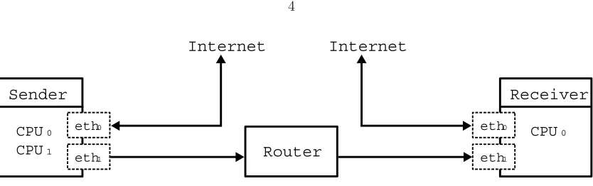
Figure 2.1: Our experimental network setup, consisting of a sender and receiver connected via an intermediary router. Link speed across our network was 10 Gigabits per second with an average round trip time of 0.057 milliseconds. Separate NICs with public IPs connecting each machine to the Internet.

a socket even while the owning process is not active. Out of context monitoring was helpful, for

example, to gain TCP window statistics. We implemented these socket and scheduler changes within

the Linux 2.6.19.2 kernel. When set, socket monitoring decreased bandwidth by approximately 3%.

To maintain accuracy, the option was set immediately prior to any calls that transmitted data, and

always by the same thread that handled I/O on the socket. It was disabled once the TCP connection

was terminated.

2.2

Experimental Setup

2.2.1

Hardware setup

Our test bed consisted of a sender and receiver connected via a Cisco 7609 Router (Figure 2.1).

Our sender and receiver had equivalent 2.4GHz 64-bit AMD processors, however, our sender had

two cores enabled, while our receiver had only one. Each machine had two Ethernet interfaces: one

connecting them to the Internet, the other connecting them to the private, experimental, network.

Their private network interface cards were Neterion Xframe II’s operating at 10Gb per second on

a 64-bit 133MHz PCI-X I/O bus. When the connection was otherwise idle, we achieved an average

ping-based round trip time of approximately 0.053 milliseconds. We used maximum transfer unit of

9000 bytes for our testing. Each machine also had 1 MB of L2 cache, and 4GB of main memory.

2.2.2

Traffic Generation

Traffic for our tests was generated using iperf.2 We altered the standard 2.0.2 version as described

inSection 2.1so that socket measurements could be made. An experiment consisted of several data

transmission sessions. For a given session, data was transferred from the sender to the receiver for

2_{iperf is a tool specifically designed “for measuring TCP and UDP bandwidth performance.” It is distributed and}

2.2.3

Background Load

To generate background load on our receiver, we used a custom application that stressed a tunable

combination of CPU and memory. In a tight loop, the application read from and wrote to random

places in a given memory area, sleeping for a given amount of time (at microsecond granularity)

between iterations. Both memory and sleep time were controlled via command line parameters.

Our application was able to allocate anywhere from 0 bytes to 200% of the system RAM amount

(going beyond 100% invoked the system pager). The sleep parameter served as a sort of CPU usage

throttle.

To simulate load within the receiving application itself, we forced the receiver to sleep between

network read calls. As with our CPU/memory application, this was controlled at microsecond

granularity.

2.3

TCP Parameters

Buffer size was controlled via the /proc file system. Among other things, the /proc file system

allows users to access kernel-level variables, including several pertaining to TCP operation. Many of

the variables within/procallow not only read access, but write access as well without interrupting

OS operation. Only a small subset of /procvariables were altered for our testing:

tcp *mem There are three TCP memory variables that affect memory usage: tcp rmem, tcp wmem,

and tcp mem. Respectively, they control memory management of TCP receive socket buffers,

send socket buffers, and the overall TCP stack size. Each variable consists of three values

the kernel interprets as minimum, maximum, and default memory levels (referred to herein as vmin,vdef, andvmax, respectively). These values act as memory bounds for dynamic allocation

of TCP related objects.

tcp rmem During each testv_min=v_def =v_maxon the receiver. This ensured internal dynamic

memory management was disabled. On the sender, v_def was larger than the maximum

receive value, and thatvmaxwas twice the value ofvdef.

3_{The application buffer should not be confused with the socket buffer. The application buffer is a concept that}

tcp wmem On both the sender and the receiver, we set v_def to be larger than the maximum

receiver buffer size andv_max= 2∗v_def. This ensured that we were not congestion window

limited.

tcp mem vmax of this variable was more than thevmax variables of tcp rmem and tcp wmem

combined.

tcp moderate rcvbuf This Boolean value is used by the kernel to turn TCP socket buffer

auto-tuning on or off. On the receiver, this was always set to “false” in order to ensure that our

requested buffer sizes were respected.

tcp no metrics save A Boolean value that controls TCP caching within the kernel. To get

consis-tent results between tests, this value was set to false on both the sender and receiver.

Chapter 3

Results

Using the methods described in the previous chapter, our goal was to determine the effects the

receive buffer has on throughput. Specifically, whether or not increased buffering at the receiver can

minimize the effects of actions adverse to receiving. We considered two cases:

1. The receiver itself was the bottleneck. In this case the receiver emulated a typical server, doing

performing work over the incoming packets.

2. The system as a whole was the bottleneck. Although the receiver was able to operate

un-hindered, the system was not entirely devoted to receiving. Instead, other applications were

running in parallel that consumed shared resources.

Our primary metric of comparison was the amount of bandwidth the TCP connection was able to

achieve at various receive buffer sizes. We also, however, look at various scheduling-based metrics

to help explain our bandwidth curves.

3.1

Working Receiver

In our working receiver tests, the receiving application was working while it received packets. To

simulate work, the receiver delayed consecutive calls to readby a given number of microseconds.1

We studied delay values ranging from 0 to 50 microseconds. The zero microsecond case represented

a non-working, uninterrupted, receiver. While a somewhat unrealistic scenario, it provided a good

baseline for comparison. Under these ideal conditions, we were able to achieve a maximum

through-put of approximately 6.66Gbps.2 From Figure 3.1(a), throughput increased with increased buffer

size. However, after a certain point (≈1 MB) this one-to-one correspondence stopped—no matter

how much larger the receive buffer size became, the number of bits transferred per second remained

constant.

1_{This was implemented using a tight loop; the application did not sleep.}

2_{Although we had 10Gb of total bandwidth available, our I/O bus limited us to 7.93Gbps. Thus, our maximum}

1 2 3 4 5 6 7

0 0.2 0.4 0.6 0.8 1 1.2 1.4 1.6

Throughput (Gbit/s)

Buffer Size (Megabytes) 0 μs

10 μs 30 μs 50 μs

(a) Throughput with receiver delay. Curves represent delay values between consecutive read calls at the receiver, in microseconds.

0 0.1 0.2 0.3 0.4 0.5 0.6 0.7 0.8 0.9 1

0 0.2 0.4 0.6 0.8 1 1.2 1.4 1.6

Fraction

Buffer Size (Megabytes) 0 μs 10 μs 30 μs 50 μs

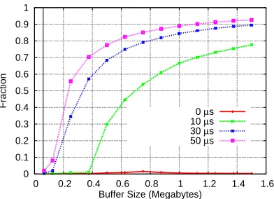
(b) Receive buffer utilization. Curves represent the percentage of buffer used with respect to the amount of buffer available.

Figure 3.1: Bandwidth and buffer utilization at increasing receive buffer sizes. The vertical line near they-axis represents the BDP based buffer size.

The amount of time spent between read calls had a dramatic affect on throughput, as seen

in Figure 3.1(a): increasing receiver delay decreased overall bandwidth. Figure 3.1(b) shows the

percentage of buffer space used at the end of the receivers active time. As the amount of time spent

by the receiver increases, so to does the amount of buffer space used. In line with our hypothesis,

TCP is trying to shield the connection from a slow receiver via buffering.

3.2

Resource Sharing

We sought to ascertain the effect of receive buffer size in the midst of background CPU and memory

load. One of the benefits of the receive buffer is that it prevents a TCP connection from collapsing

during periods of bursty traffic; we want to know whether the same can be said for periods of high

system load. As mentioned inSubsection 2.2.3, we used a custom application to generate CPU and

memory load. In these tests, the receiver did no processing of incoming packets.

3.2.1

Memory

First, we considered the affect memory allocation had on bandwidth. For our experiments, we

con-sidered between 1 and 150 percent system memory allocations; roughly 41MB and 6GB, respectively.

From Figure 3.2(a), while memory allocation did have an affect on perceived throughput, receive

buffer size did not help. If our initial hypothesis was correct, the correspondence between buffer

1 2 3 4

0 0.2 0.4 0.6 0.8 1 1.2 1.4 1.6

Throughput (Gbit/s)

Buffer Size (Megabytes) 1% 99% 150%

(a) Throughput at various memory utilization. Lines represents the percentage of system memory (4GB) used.

1 2 3 4

0 0.2 0.4 0.6 0.8 1 1.2 1.4 1.6

Throughput (Gbit/s)

Buffer Size (Megabytes) 0 μs 10 μs 100 μs

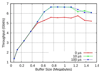
(b) Throughput at various background CPU utiliza-tion. Each line is the amount of time our background load application slept between successive operations.

Figure 3.2: Bandwidth observed by our receiving application as it shared different system memory and CPU. In neither case did the size of the receive buffer play a role in shielding the receiver from the effects on the background load.

memory allocated. That is, if ri represents the optimal buffer size3 with i% of system memory

consumed, then the following relation should have held: r₁ < r₉₉ < r₁₅₀. In reality, when 99% of

the system memory was utilized, a receive buffer of approximately 768KB was optimal—the same

buffer that was optimal in the 1 and 150% memory utilization cases.

As an aside, we consistently observed that the relationship between memory usage and

through-put was not completely linear: bandwidth at 150% memory utilization is better than bandwidth

experienced when 99% of the memory was used—a counter intuitive observation. Our memory

ap-plication was independently verified, so we assume the effect to be an artifact of the Linux paging

system.

3.2.2

CPU

Our hypothesis was also tested against CPU sharing. To conduct the experiments, our memory

ap-plication slept between successive memory accesses. Sleeping for zero seconds caused the apap-plication

to become not only memory bound, but CPU bound as well, as it had to calculate the array offsets.

This effect was minimized by sleeping for longer periods of time between loop iterations. We studied

sleep values between 0 and 100 microseconds. Results from these tests can be seen inFigure 3.2(b).

As was the case in our memory testing (Subsection 3.2.1), the receive buffer was unable to shield

the receiver from the effects of processor sharing. In this case, the optimal buffer size was the same,

irrespective of background load.

0

1

2

3

4

5

6

7

0

0.2

0.4

0.6

0.8

1

1.2

1.4

1.6

Throughput (Gbit/s)

Buffer Size (Megabytes)

-20

0

12

15

19

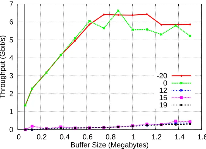
Figure 3.3: Bandwidth of priority sharing.

3.2.3

Priority

Finally we studied how a processes priority affected bandwidth and resource sharing. Tests were run

in the same fashion as described inSubsection 3.2.2, however, the priority of the receiving application

was varied. More specifically, we ran our receiving application in conjunction with the background

load generator, which used 99% of the system memory and did not sleep between memory accesses.

Linux assigns priorities to processes with what is known as anice value—the “nicer” a process, the

more willing it is to share the CPU. Thus, high priority processes have negative nice values, while

low priority processes have higher nice values. By default, processes have a nice value of 0. In the

case of our experiments, the priority of our background application remained constant at its default

value. The priority of our receiving application varied, however, between minimum and maximum

Linux nice values of -20 and +19.

Overall, and in line with theory [3], scheduling priority had the most notable effect on throughput

in all of our background load tests; results can be seen inFigure 3.3. The default priority allowed

our receiving application to be hampered somewhat. At the highest priority however, maximum

bandwidth was achieved irrespective of the background load.

In line with our hypothesis, buffering did have an effect on throughput, albeit slight. When the

receiving application was assigned a low priority there was a linear relation between buffer size and

Chapter 4

Conclusion

Linux does a very good job, overall, of getting data from the network card to the receiver. Under

ideal conditions, data was transferred from internal buffers to the application within the application

context. We found that usage of the receive buffer only became noticeable when the receiving

application was internally hindered; when it had to both receive and do work. External factors, such

as resource sharing amongst other applications, had an adverse affect on throughput; contrary to

our hypothesis, however, receive buffer size did nothing to improve this perceived throughput.

4.1

Future Work

4.1.1

Networking disconnect

As mentioned inSection 3.1if the receiver had more than a few microseconds worth of work on the

received data, the relationship between buffer allocation and buffer used became linear. That is, the

more space available to TCP, the more space it used. Unfortunately, this relation did not carry over

to throughput—TCP was able to get the same amount of throughput using much less buffer space.

We think of this as a disconnect between TCP and the receive buffer. The operating system should

not use all available resources just because it can.

This problem could probably be solved by increasing the amount of feedback between TCP and

the application. The current Linux kernel is able to do receive aware auto-tuning, which is a step in

this direction. Currently, the kernel keeps track of the amount of time a packet is in the TCP receive

state—the time difference between a packet being put in the receive queue and that same packet

being delivered to the application. The shortcoming we notice, however, is more so in the length

of time between packet delivery and subsequent packet transmission. We are not out to improve

4.1.2

Logarithmic throughput

During the course of testing, several interesting, but somewhat tangential observations were made.

One such observation that warrants further investigation is the effect of the maximum transfer unit

(MTU) on bandwidth at varying receive buffer sizes. It is well known, and confirmed with our own

testing, that MTU plays a large role in the maximum achievable throughput between two points.

We also observe that the buffer size required to achieve that maximum throughput is logarithmically

dependent on the MTU. Some have speculated that this phenomenon is a result of Linux memory

management [1]; however, that has not been definitively proven, nor formally modeled. Having an

Bibliography

[1] Wu chun Feng, Justin (Gus) Hurwitz, Harvey Newman, Sylvain Ravot, R. Les Cottrell, Olivier

Martin, Fabrizio Coccetti, Cheng Jin, Xiaoliang (David) Wei, and Steven Low. Optimizing

10-gigabit Ethernet for networks of workstations, clusters, and grids: A case study. In 2003

ACM/IEEE conference on Supercomputing, page 50, Washington, DC, USA, 2003. IEEE

Com-puter Society. 4.1.2

[2] Eric Weigle and Wu-chun Feng. A comparison of TCP automatic tuning techniques for

dis-tributed computing. In 11th IEEE International Symposium on High Performance Distributed

Computing HPDC-11 2002 (HPDC’02), page 265, Washington, DC, USA, 2002. IEEE Computer

Society. 1

[3] Wenji Wu and Matt Crawford. Performance analysis of Linux networking packet receiving. In