Assessing the effect of stellar companions from high-resolution imaging of Kepler objects of interest

Assessing the Effect of Stellar Companions from High-resolution Imaging of

Kepler

Objects of Interest

Lea A. Hirsch1, David R. Ciardi2, Andrew W. Howard3, Mark E. Everett4, Elise Furlan5, Mindy Saylors2,9, Elliott P. Horch7, Steve B. Howell8, Johanna Teske6, and Geoffrey W. Marcy1

1

University of California, Berkeley, 510 Campbell Hall, Astronomy Department, Berkeley, CA 94720, USA;[email protected]

2

NASA Exoplanet Science Institute Caltech-IPAC, Pasadena, CA 91125, USA

3

California Institute of Technology, Department of Astronomy; MC 249-17, Caltech, Pasadena, CA 91125, USA

4

National Optical Astronomy Observatory, 950 N. Cherry Avenue, Tucson, AZ 85719, USA

5

Caltech-IPAC, Mail Code 100-22, Caltech, 1200 E. California Boulevard, Pasadena, CA 91125, USA

6

Carnegie DTM, 5241 Broad Branch Road, NW, Washington, DC 20015, USA

7

Southern Connecticut State University, Dept of Physics, 501 Crescent Street, New Haven, CT 06515, USA

8

NASA Ames Research Center, Moffett Field, CA 94035, USA

9

College of the Canyons, 26455 Rockwell Canyon Road, Santa Clarita, CA 91355, USA

Received 2016 July 5; revised 2016 November 29; accepted 2017 January 13; published 2017 February 20

Abstract

We report on 176 close(<2″)stellar companions detected with high-resolution imaging near 170 hosts ofKepler Objects of Interest (KOIs). TheseKeplertargets were prioritized for imaging follow-up based on the presence of small planets, so most of the KOIs in these systems(176 out of 204)have nominal radii<6RÅ. Each KOI in our

sample was observed in at least twofilters with adaptive optics, speckle imaging, lucky imaging, or theHubble Space Telescope. Multi-filter photometry provides color information on the companions, allowing us to constrain their stellar properties and assess the probability that the companions are physically bound. We find that 60%–80% of companions within 1″are bound, and the bound fraction is>90% for companions within 0 5; the bound fraction decreases with increasing angular separation. This picture is consistent with simulations of the binary and background stellar populations in the Keplerfield. We also reassess the planet radii in these systems, converting the observed differential magnitudes to a contamination in theKeplerbandpass and calculating the planet radius correction factor, XR=Rp(true)/Rp(single). Under the assumption that planets in bound binaries are equally likely to orbit the primary

or secondary, we find a mean radius correction factor for planets in stellar multiples of XR = 1.65. If stellar

multiplicity in theKeplerfield is similar to the solar neighborhood, then nearly half of allKeplerplanets may have radii underestimated by an average of 65%, unless vetted using high-resolution imaging or spectroscopy.

Key words:binaries: visual –planets and satellites: detection–planets and satellites: fundamental parameters– techniques: high angular resolution– techniques: photometric

Supporting material:machine-readable tables

1. Introduction

During the four year tenure of theKeplermission, over 4000 planet candidates (PCs) were identified and their radii estimated. The size of the Kepler sample allows for detailed population statistics to determine the occurrence rates of planets of various sizes and orbital distances. Of primary interest is a determination of the occurrence rate of small planets, especially those with radii smaller than 1.6RÅ, which

could potentially be rocky (Lopez & Fortney 2014; Marcy et al.2014; Rogers2015). The transition from“non-rocky”to

“rocky” planets appears to be extremely sharp, making the detection of accurate planet radii critical for occurrence rate analyses(e.g., Ciardi et al.2015; Rogers2015)

Planet radius estimates fromKeplerlight curves rely on the inferred properties of the planet host star. Due to the fairly low resolution and large pixel scale of the Keplerdetector, stellar companions are difficult to detect without ground-based follow-up observations. Higher-resolution imaging provides the most efficient method for detecting line-of-sight and bound companions within 1″. These companions, if present, can dilute the Kepler light curves, preventing an accurate assessment of the planet radius.

In the solar neighborhood, at least 46% of Sun-like stars have bound stellar companions(Raghavan et al.2010), with the

orbital separation distribution peaking at50 au. Assuming the Keplerfield has similar multiplicity statistics, nearly half of the Keplertarget stars could have bound stellar companions falling within the sameKeplerpixel.

Unknown close stellar companions will cause planetary radii to be underestimated, depending on the relative brightness of the binary components, and which star the planet is orbiting. For faint companions to planet hosts, the contamination from the secondary component may be limited to only a few percent; however, if the planet is determined to be orbiting the fainter secondary component, the planet radius estimate could be off by an order of magnitude(Ciardi et al. 2015). Unfortunately, determining which star in a binary pair hosts the observed transiting planet is not straightforward, and requires extensive individualized statis-tical modeling(e.g., Barclay et al. 2015).

Neglecting to account for stellar multiplicity can have ramifications for the accuracy of occurrence studies of small planets. Since unknown stellar companions can cause larger planets to masquerade as “small”planets, stellar companions can artificially boost estimates of small planet occurrence by as much as 15%–20% (Ciardi et al. 2015). High-resolution imaging follow-up is therefore extremely important for obtaining accurate measurements of planet radii.

Binary companions may also affect the formation and evolution of planets in a stellar system, and planets in binary systems are therefore an interesting sub-sample of the wider Kepler sample. The full implications of stellar multiplicity on planet formation and evolution are still being explored. Previous studies (e.g., Wang et al.2014b; Kraus et al. 2016) indicate that stellar multiplicity may be suppressed in planet-hosting Kepler systems, compared to field stars in the solar neighborhood (Raghavan et al.2010). This may indicate that planet formation is rarer in close binary systems than in single-star systems. If this is the case, the problem of transit dilution from unknown stellar companions may impact fewer systems than expected based onfield star multiplicity statistics.

On the other hand, stellar multiple systems contain more than one star to host potentially discoverable planets, so their number may be enhanced in the Kepler Object of Interest (KOI) sample. Additionally, the augmented brightness of unresolved binaries relative to single stars of the same spectral type allows the flux-limited Kepler survey to include stellar multiples at larger distances than corresponding single-star systems. This might also augment the expected number of Kepler systems in which flux dilution plays a role. The combined result of these various effects is complex, and more detailed statistical work on Kepler binary statistics is still needed.

TRILEGAL galactic models with assumed multiplicity statistics were applied to theKeplerfield in order to determine the likelihood of chance alignments with background stars. These models indicate that companions observed within 1″of a KOI are highly likely to be bound companions, and therefore potentially play a dynamical role in the formation and evolution of the stellar system (Horch et al. 2014). More specifically, companions within 0 4 have a less than 10% likelihood of being chance background alignments, and companions within 0 2 have a nearly zero percent chance, based on the TRILEGAL galaxy models.

We study KOI host stars with detected close (<2″) companions on a case-by-case basis, in comparison to the statistical study performed by Horch et al.(2014). In Section2, we discuss the stellar sample of KOI hosts chosen for this study. In Section 3, we describe the Dartmouth isochrone models used to determine whether a companion is physically associated based on color information, and the TRILEGAL models used to assess the background stellar population. In Section 4, we isolate a population of KOI hosts with bound companions and compare the bound fraction as a function of separation to the simulation results of Horch et al. (2014). Finally, in Section5, we calculate radius correction factors for all of the PCs and many of the confirmed planets in our sample for use in future occurrence studies.

2. Sample

2.1. KOI Host Stars

Our sample consists of 170 stellar hosts of KOIs observed with various high-resolution imaging campaigns. This sample was drawn from the overall sample of KOI stars observed with high-resolution imaging, described in the imaging compilation paper by Furlan et al. (2017, hereafterF17).

We choose targets for this study by requiring that at least one companion was detected within 2″, and that the companion was detected in two or morefilters, providing color information. We

choose the 2″separation limit to include all companions falling on the sameKepler pixel as the primary KOI host star. For a complete list of detected companions, see F17. Because imaging campaigns typically targeted the hosts of small planets, our sample contains a high fraction of small planet hosts.

Figure1is a histogram of the apparentKeplermagnitudes of our sample KOI hosts in comparison with the full ensemble of KOI stars followed up with high-resolution imaging, described inF17. Although some efforts were made to image very faint Kepler targets, none of our sample stars have Kepler magnitudes fainter than 16. The majority of small Kepler planets orbit faint host stars; however, this difficulty is currently remedied by theK2and upcomingTESSmissions.

For each stellar primary, the parameters Teff, logg, and

[Fe/H] are taken from Huber et al.(2014). For many of the stars in our sample (71), these parameters come from spectroscopic or asteroseismic analysis performed by Huber et al.(2014,2013), Chaplin et al.(2014), Ballard et al.(2013), Mann et al. (2013), Batalha et al. (2013), Buchhave et al. (2012), and Muirhead et al. (2012). The spectroscopic and asteroseismic analyses provide stellar parameters largely unaffected by interstellar extinction toward the Kepler field. These techniques are also largely unaffected by undetected close stellar companions, unless the companions’spectral lines contaminate the primary stellar spectrum to a significant degree.

The remaining sample stars have stellar parameters calcu-lated from photometry, reported in Huber et al. (2014). Of these, all but 13 have properties revised by Pinsonneault et al. (2012), Gaidos (2013), or Dressing & Charbonneau (2013), using new models and data to improve on the originalKepler Input Catalog(KIC)stellar parameters. For the purposes of our study, we do not re-analyze the stellar properties of any stars in

our sample. Rather, we take the primary stellar properties from Huber et al. (2014) as given, and assess the characteristics of the companions detected around these stars.

For the 13 stars with KIC stellar parameters, the latter are expected to be more uncertain than for stars with parameters derived from seismology, spectroscopy or improved photo-metric relationships. Additionally, in the case of systems with nearby companions, the photometry might be contaminated by the blended companion. The photometrically derived stellar properties may therefore be biased. While we recognize this possible effect, it is beyond the scope of this paper to fully re-derive the stellar parameters for the primary stars, especially in light of the fact that many of the stars have parameters derived from spectroscopic and seismological observations.

Figure 2 shows the distribution of stellar Teff, logg, and

[Fe/H]of our sample stars. The stars in this work are primarily G and K dwarfs, but the sample also includes 13 stars with

Teff<4000 K, and six hot stars withTeff>8000 K. We also

include four evolved stars withlogg<3.5(see Figure3). Our sample contains 110 confirmed planets in 72 systems. Of these, 15 planets are confirmed including analysis of high-resolution imaging observations, allowing the authors to correct for the multiplicity of the host stars. These, we continue to treat as confirmed, and we do not reanalyze the planetary parameters. However, the remaining 57 systems were con-firmed without the input of observations sensitive to stellar companions, so we do include these systems in our planet radius reanalysis. Eight of these systems were confirmed by nature of multiplicity by Rowe et al. (2014), since transiting multi-planet systems have very low statistical probability of displaying false positive(FP)signals in addition to true planets. Morton et al. (2016) confirm 45 systems using statistical arguments where the possibility of the planets orbiting a secondary star within a stellar binary system was explicitly neglected. Finally, two systems were confirmed by Van Eylen & Albrecht (2015) and three were confirmed by Xie (2013, 2014) using Transit Timing Variation (TTV) analysis to confirm multi-planet systems. For these 57 systems, the high-resolution imaging follow-up data available to the public on the ExoFOP10 were not employed prior to confirmation, nor was the possibility of planets orbiting a stellar companion

addressed. We therefore include these systems in our radius update analysis, while excluding confirmed systems with extensive analysis of high-resolution imaging data carried out by other groups.

Of the target systems, 76 have one or more PC, including many of the systems which also host confirmed planets. There are a total of 94 PCs in the sample. There are also 36 systems which host 38 FP signals, including a few which also have PCs or confirmed planets. These systems were followed up with high-resolution imaging prior to receiving a FP disposition. We assess whether the stellar companions of these systems are bound, but we do not include these transits in our analysis of planet radius updates in Section5. Thirty nine KOI stars in our sample host multi-planet systems, with 105 total planets or PCs among these systems.

It is important to note that the official Kepler project used none of the ExoFOP10data(e.g., images)to assess candidates

Figure 2.Histograms of stellar parametersTeff,logg, and[Fe/H]from Huber et al.(2014)for stars in our sample. The majority of our sample stars haveTeff<7000 K

andlogg>4.0. We includefive stars that may be subgiants based on their reportedloggvalues(logg<3.5), as well asfive hotter stars(Teff>8000 K).

Figure 3.HR diagram of target KOI primary stars based on their stellar properties from Huber et al.(2014). Dartmouth isochrones are displayed for context, spanning ranges in metallicity from−2.4 to+0.5(in steps of 0.1 dex) and age from 1.0 to 15.0 Gyr(in steps of 1 Gyr).

10

or FPs in the published PC catalogs(e.g., Batalha et al.2013; Burke et al. 2014; Rowe et al.2015; Mullally et al.2015).

2.2. Stellar Companions

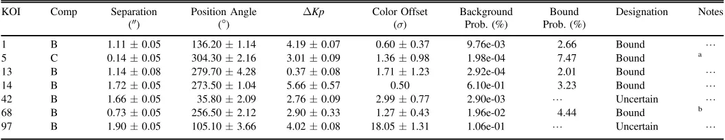
Table 1 documents the observations of companions to our KOI host star sample, compiled from the imaging compilation paper ofF17. Columns(1)and(2)provide the KOI number and component of the companion. Columns(3)and(4)describe the companion’s position relative to the KOI primary star, and column (5) describes the differential magnitude between the primary star and companion in theKepler bandpass,ΔKp, all taken from F17. Columns (6)–(8) provide data leading to a determination of bound, uncertain, or unbound for each companion(9), which is explained in Section 3.

F17 details the observations and measured differential magnitudes (Δm=m2-m1) for stars with high-resolution

imaging, including our target systems. Each companion within 2″must have at least two measuredΔmvalues from the full set of filters used for follow-up observations, in order to be included in our sample. These filters include J-band, H-band, and K-band from adaptive optics imaging from the Keck/ NIRC2, Palomar/PHARO, Lick/IRCAL, and MMT/Aries instruments; 562, 692 and 880 nmfilters from the Differential Speckle Survey Instrument (DSSI) at the Gemini North and WIYN telescopes; i and z bands from the AstraLux lucky imaging campaign at the Calar Alto 2.2 m telescope(Lillo-Box et al. 2014); and LP600 and ibands from Palomar/RoboAO (Law et al.2014). We also include seeing-limited observations in the U-, B-, and V-bands from the UBV survey (Everett et al.2012)and “secure”detections(noise probability<10%) in theJ-band from the UKIRTKeplerfield survey.

In several of our higher-order multiple systems, only one component has detections in multiplefilters, often due tofi eld-of-view cutoffs or non-detections of very faint companions. We describe these additional companions in the notes section of the Appendix, and include them in the planet radius correction, but cannot include them in our physical association analysis.

Figure 4 displays the separation versus Δm measured for each companion detected within 2″of our sample KOI stars in the DSSI, Astralux, RoboAO,UBV, and AOfilters(seeF17).

It is important to note that the term“companion”is used here to describe any star detected angularly nearby a KOI host star. It is not used to imply physical association. Instead, we will refer to physical binary or multiple systems as “bound” companions, and unphysical, line-of-sight alignments as

“unbound”or“background”companions.

3. Determining Physical Association of Companion Stars

Detection of a stellar companion near a KOI host star does not necessarily imply that the system is a physical binary. An assessment of the companion’s stellar properties must be made to determine if the detected companion is physically bound, or simply a line-of-sight alignment of a background or foreground star. If the system is found to be a bound binary, then the companion may have played a dynamical role in the evolution of the planetary system; additionally, the planets may orbit either of the two stars in the system. If an unbound companion, only theflux dilution from the background source can be taken into account.

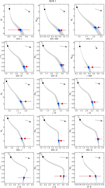
We use the Dartmouth Stellar Evolution models (Dotter et al. 2008) to assess whether each detected companion is consistent with the isochrone of its respective primary star, by comparing the measured color to that predicted for a model bound companion. This technique has been employed in previous works by Everett et al.(2015), Teske et al.(2015), and Wittrock et al.(2016). We provide samplefigures to elucidate this process in Figures5 and6, choosing one unambiguously bound companion(KOI 1 B), and one unambiguously unbound companion (KOI 3444 F) to clarify the technique. Note that KOI 3444 F, at a separation of 3 5, is not included in our 2″ sample, and was predicted to be unbound prior to analysis due to its larger angular separation from its primary KOI star. Not all companions have data available in as many colors as these two stars; many have only a single plot panel(onefilter pair). A description of our technique and cutoffs follows.

1. We use the Dartmouth models to produce a set of isochrones spanning ranges in metallicity from −2.5 to

+0.5(in steps of 0.02 dex)and age from 1 to 15 Gyr(in

Table 1

Observed Companions of the KOI Host Sample

KOI Comp Separation Position Angle ΔKp Color Offset Background Bound Designation Notes

(″) (°) (σ) Prob.(%) Prob.(%)

1 B 1.11±0.05 136.20±1.14 4.19±0.07 0.60±0.37 9.76e-03 2.66 Bound L

5 C 0.14±0.05 304.30±2.16 3.01±0.09 1.36±0.98 1.98e-04 7.47 Bound a

13 B 1.14±0.08 279.70±4.28 0.37±0.08 1.71±1.23 2.92e-04 2.01 Bound L

14 B 1.72±0.05 273.50±1.04 5.66±0.57 0.50 6.10e-01 3.23 Bound L

42 B 1.66±0.05 35.80±2.09 2.76±0.09 2.99±0.77 2.90e-03 L Uncertain L

68 B 0.73±0.05 256.50±2.12 2.90±0.33 1.27±0.43 1.96e-02 4.44 Bound b

97 B 1.90±0.05 105.10±3.66 4.02±0.08 18.05±1.31 1.06e-01 L Uncertain L

Note.Tabular summary of companions to KOI host stars in our sample. Columns(1)–(4)describe the positions of the companions, taken fromF17. Column(5) describes theΔmin theKeplerbandpass between the primary and companion, taken fromF17for uncertain and unbound companions, and from our isochrone models for the bound companions. Columns(6)–(9)describe the physical association assessment, described in Section3. In brief, the color offset(6)indicates the difference, in units of the model and measurement uncertaintyσ, between the modeled and observed colors of the companion. Better agreement means the companion is more likely to be physically bound. The error quoted for color offset is its standard deviation, which describes the variation in the color offset among several differentfilter pairs. Systems with only a single color measurement have no reported standard deviation. Systems with poor agreement have higher color offset standard deviation, and are likely to be reclassified as uncertain. Background probability(7)and bound probability(8)refer to the analysis using TRILEGAL galaxy models(Girardi et al. 2005)and solar neighborhood stellar multiplicity statistics(Raghavan et al.2010)respectively, in Section3.2. Notes on additional companions to individual systems, marked with letters in Column(10), can be found in theAppendix.

steps of 0.5 Gyr). We further interpolate these isochrones to achieve sampling in stellar mass between 0.1 and 4M, with intervals no larger than 0.02M. We also

incorporatefilter transmission curves for the DSSIfilters, allowing absolute magnitudes to be predicted in these filters from the isochrone models.

2. We use the primary stellar parameters Teff, logg, and

[Fe/H]from Huber et al.(2014)to place the primary KOI host star on the isochrones and calculate a probability distribution for the primary star absolute magnitude in each of thefilters in which that star was observed. Note that these distributions are subject to inaccuracy for the 13 stars with original KIC photometrically derived stellar properties which, if bright, are likely to be more evolved than predicted by the original KIC.

3. To compute the observed colors of the detected companions, we add the measured Δm values to the modeled absolute magnitudes of the primary stars, and subtract in pairs. This is particularly important for the stars detected with speckle imaging, since the DSSIfilters are non-standard, and are not calibrated against more commonly used filters. We therefore have no measured apparent magnitudes for the primary stars in thesefilters, from which we could deblend the component stars. Thus we use the isochrone magnitude of the primary to derive a magnitude of the companion from the observedΔm, then derive colors from the pairs offilters. For uniformity, we use this technique for all colors, even those including standard filters only (e.g., J−K), where observed apparent magnitudes could be used.

4. We compute isochrone models for a bound stellar companion using each measured Δm. We propagate the primary star’s probability distribution down the set of applicable isochrones by the measured Δm value. This provides an estimate of the stellar parameters of a bound stellar companion with the measuredΔm. Each companion hasn“isochrone-shifted”models, wherenis the number of filters in which it is detected (at least two for each companion). We average these n models to obtain a weighted-average bound companion probability distribution. 5. For each pair of applicable filters, we calculate the probable color of a hypothetical bound companion. We then compare this model color with the observed color of the companion to assess whether the companion is consistent with being bound. For a companion with Δm measurements innfilters, we can calculate n n( -1)

2 colors.

We use the weighted average companion model (which takes into account each measured Δm) to predict the model colors for every possible color pairing. We calculate the offset between model and observed color for each color pair, in units of the uncertainties in the measurements and models.

For a set of observations for a given star, the measured colors are not necessarily independent of each other(e.g.,

( ) ( )

- = - +

-J K J H H K ). However, to help miti-gate the effects of using any one specific filter over the others, we have generated all possible colors for thefilters available to assess the agreement between the observed and isochrone-model colors for each companion.

6. We take the average color offset between the models and observed colors, weighting by the measurement and model uncertainty in the two relevant filters for each

color. This average color offset(as well as the weighted standard deviation of color offset)is provided in column (6)of Table1. If the average color offset is less than 3σ, we designate the companion as bound. If it is greater than 3σ, we designate the companion as unbound.

7. We isolate and reclassify systems where the designation is uncertain. First, we look for companions whose bound/ unbound designation is reliant on a single, very significantΔmmeasurement. We re-calculate the average color offset, removing the most significant observed color. If this procedure changes the conclusion, we reclassify the system as uncertain. Additional refinement of theΔmmeasurements is needed to determine whether the companion is bound or not.

8. Next, we look for systems with large color offset standard deviations, indicating that the conclusions from each color pair are mutually inconsistent for a single companion. If the conclusion can be changed by more than 0.5σby adding or subtracting the standard deviation from the average color offset(i.e., a seemingly unbound companion witháoffsetñ - soffset<2.5s or a seemingly

bound companion with áoffsetñ +soffset>3.5s), we

reclassify the system as uncertain.

In Figures5and6, we plot a representative set of isochrones, with[Fe/H]within±1σof the primary star’s input metallicity. In black, we plot the probability distribution of the primary star in color–magnitude space, based on the isochrone models for the primary star. Error bars indicate the ±1σ uncertainty contours.

Figure 4.Separation vs.Δmfor each companion detected within 2″of our sample KOI stars. Color denotes thefilter in which observations were made:U,

The n “isochrone-shifted” companion probability distribu-tions are plotted in light blue, with the weighted average companion model in dark blue. Finally, we plot the measured companion color in red. The horizontal error bars on the observed color represent the measurement uncertainty in the

Δmvalues used to calculate these colors. Fornfilters, we have ( - )

n n 1

2 panels in our plot, representing the number of color

combinations possible with the set of filters available. Our analysis determines that KOI 1 B is consistent with being a bound companion, while KOI 3444 F is clearly unbound.

The reader should note that this analysis makes the implicit assumption that the companion detected by each method is not itself an unresolved multiple. If a companion is itself an unresolved pair (i.e., a hierarchical multiple system), the observed Δmvalues would refer to the composite light from the companions, and the analysis may fail to accurately assess either companion star individually.

3.1. Interstellar Extinction

Our approach makes the implicit assumption that the companion is subject to the same interstellar extinction as the primary star. We check for consistency between the model and observed companion colors under this assumption.

Differential extinction between the primary and companion may cause the measured color to differ significantly from the color expected under the model assumptions, causing our analysis to produce a designation of unbound. Since the most likely scenario for producing this differential extinction is that the companion is more distant than the primary KOI star, and is therefore only a line-of-sight optical double, we would correctly conclude that the companion is unbound.

One potential source for a false negative—a bound companion that fails to satisfy our bound criteria—is a bound companion with a significant dusty envelope or disk, causing distance-independent differential extinction of the companion. However, this scenario is highly unlikely, as the target stars are not expected to be young, so should not retain their natal dusty disks.

Likewise, a plausible source for FPs would be a background object that is attenuated and reddened until consistent with the isochrone of the primary star. To provide an indication of the direction and magnitude of the effect of extinction on background companions, we have plotted an extinction vector on each panel of Figures 5 and6. These vectors have lengths corresponding to one magnitude of extinction in the V-band. Typical models of interstellar extinction toward theKeplerfield assume 1 mag of extinction inVfor every kpc of distance in the galactic plane, with extinction diminishing as a function of galactic latitude with an e-folding scale-height of 150 pc (Huber et al.2014).

While these possibilities exist, we do not have enough data to make the assessment of whether the scenarios described apply to any of our systems. Spectroscopic data would provide more information about the intrinsic properties of the companion stars, and would allow a more conclusive assessment of whether the companions are indeed bound. However, spectroscopy is not available (and is largely precluded by magnitude limits and the closeness of the stellar primary) for the vast majority of the companions included in this sample. Instead, we look at the predicted population of background stars to determine the probability that each candidate bound companion is a line-of-sight alignment. We

compare this to the probability of a solar-type primary hosting a bound stellar companion at the predicted mass ratio and separation.

3.2. Comparison with Stellar Population Models

For the companions in our sample with colors consistent with the same isochrone as the primary (candidate bound companions), we additionally check the relative probabilities of the companions being bound versus background alignment, before applying the designation of bound. Specifically, we use the known multiplicity statistics of the solar neighborhood from Raghavan et al.(2010)to determine the probability of a solar-type star having a companion within±3σ of the model mass ratio from the isochrone models, and at a separation greater than the derived projected separation.

Based on the Raghavan et al.(2010) multiplicity statistics, we utilize a log-normal distribution for the probability distribution in orbital period, which we calculate based on the observed angular separation, the predicted stellar distances from the ExoFOP website,10and the modeled stellar masses of both the primary and stellar companion. The distance estimates to each KOI star found on the ExoFOP website10derive from models calculated by Huber et al.(2014). The uncertainties on these distance estimates are typically of order 15%, and are uncorrected based on the discovery of a stellar companion. For KOIs with a bright stellar companion increasing the inferred brightness of the primary star, the true distance may be larger than the distance reported by the Huber et al.(2014)models. Greater distances would imply larger projected separations, and would therefore decrease the probability that the companion is bound.

To determine the probability of a companion within±3σof the modeled mass ratio, we assume aflat distribution in mass ratioqfrom values of zero to unity(Raghavan et al.2010). We integrate under the curve from the lower to upper bound, and apply this fraction to the overall fraction of Sun-like stars with one or more stellar companions, 46%. We then apply the fraction from integrating under the log-normal curve in orbital period, from the calculated period to infinity. We choose this upper bound to account for projection effects, allowing long orbital periods to appear as smaller separations due to orbital orientation and phase.

We note that choosing the multiplicity statistics from Raghavan et al. (2010) may not be accurate for this sample, as previous work on the Kepler field planet host stars has shown that stellar multiplicity may be affected by the presence of planets (Wang et al. 2014a, 2014b; Kraus et al. 2016). However, the specifics of this multiplicity effect are not yet well understood, so we default to using the known multiplicity statistics of the solar neighborhood.

the stellar companion, since only stars with similar brightnesses and colors to the observed stellar companions would have been consistent with our initial check against the primary star’s isochrone. We then calculate the stellar density of the field surrounding the KOI, and multiply by the area within the observed angular separation of the companion to determine the probability of a background interloper with the required brightness falling within the required area around the KOI.

We use only the Keplerbandpass tofilter the results of the galactic models, and still find background probabilities of

<12% in all cases, and<2% in all but three cases. These very low background probabilities are expected, due to the very small angular region in which all of our observed companions reside. We find similar background probabilities for stellar companions designated as uncertain and unbound based on isochrone models, with no distinct difference among the three samples. These probabilities would be further reduced if we filtered the galactic models for consistency with all measured magnitudes or colors, instead of only looking at the Kepler apparent magnitude.

Figure 7.Top: stellar properties derived from isochrone models for the bound companions to KOI stars in our target sample are plotted in the diagonally hatched red histograms. The dark blue hatched histograms show the stellar properties of the primary KOI stars in each of these bound systems for reference. As expected, companion temperatures are skewed cool, with most companions having Teff<6000 K. These companions all appear to be main sequence stars, with

 g

We calculate the ratio of bound probability to background probability for the candidate bound companions. In all but two cases, these ratios exceed unity, typically by one or more orders of magnitude. The median value of the probability ratio for stars in the bound category is 367.5. Only 11 stars have probability ratios less than 10, and only two(KOI 703 B and and KOI 6425 B)have ratios less than unity. We move these two companions to the uncertain category, and do not include them in any further analysis of bound systems. In Table1, we provide the background probabilities, based on the TRILEGAL models, for all companions. We also provide the bound probabilities based on multiplicity statistics of the solar neighborhood (Raghavan et al. 2010) for the companions consistent with being bound.

4. Bound Companions toKeplerPlanet Hosts

Based on the isochrone analysis and comparison to background stellar population models, we highlight a popula-tion of KOI hosts with likely bound companions, listed in Table1. This group of planet-hosting stellar multiple systems is a valuable comparison sample for the widerKeplerplanet host population.

We plot the distributions of stellar properties for the bound companions to our sample targets in Figure7. We also plot for reference the stellar parameters of the primary stars in these bound binary systems. The companion population has a lower averageTeff and a higher averageloggthan their primary stars,

as expected for a coeval pair. The bottom panels of Figure 7 show the radius and mass ratios of the bound stellar companions. This information feeds directly into the planet radius correction factors, described in Section5. Note that this distribution is subject to detection limits on much fainter companions, so the lower number of stellar companions at small radius and mass ratio likely reflects the difficulty in detecting high-contrast systems. Malmquist bias may also play a role, since systems with mass and radius ratios close to unity would be brighter, and therefore overrepresented in both the Keplersample and the subsample of stars with high-resolution imaging follow-up.

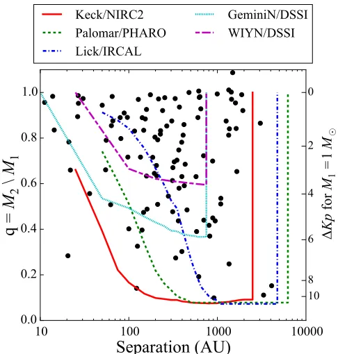
In Figure 8, we plot the projected physical separations and mass ratios of each bound multiple system, in order to demonstrate the sensitivity of high-resolution imaging cam-paigns to companions in physical space. We calculate projected separation using the distance estimates to each KOI star found on the ExoFOP website.10The uncertainties on these distance estimates are typically 15%–20%. Since the stellar companions to all of these KOI stars may increase the apparent brightness, stars with companions may be more distant than the models indicate, and the true projected separations may therefore be correspondingly larger. Mass ratios are calculated based on the isochrone models for each component of the system.

For reference, we provide characteristic detection limits for each of several techniques used tofind the stellar companions here. We include AO observations from Keck/NIRC2, Palomar/PHARO, and Lick/IRCAL, as well as DSSI speckle observations from the Gemini North and WIYN telescopes, taken fromF17. We convert these detection limits from angular separation and Δm to projected separation and mass ratio by assuming the primary star is a solar-mass star at a distance of 500 pc. These are typical values for the primary stars in our sample, which have a median temperature of 5780 K and a median distance of 420 pc. Note that the exact detection limits

will differ for each KOI system based on its primary star mass and distance.

In the future, the distribution of stellar systems in this diagram could be compared to a theoretical distribution, based on known properties of solar neighborhood binaries (e.g., Raghavan et al.2010), typical stellar properties and distances to stars in theKeplerfield, and the detection limits of each of the techniques used here. This comparison would allow us to test whether the multiplicity ofKeplerplanet hosts is qualitatively similar to typical field binaries. However, this analysis is outside the scope of this paper, which is primarily focused on determining whether the companions discovered by high-resolution imaging are bound or not. For an ideal statistical study of stellar multiplicity as it relates to planet occurrence, a more careful selection of a target stellar sample, as well as a control sample, is required.

Horch et al. (2014) simulate the binary and background stellar populations for the Kepler field, and conclude that within the detection limits of the DSSI instrument at either the WIYN 3.5 m or Gemini North telescopes, the vast majority of sub-arcsecond companions detected with high-resolution imaging should be bound, rather than line-of-sight companions. The bound fraction versus separation curve depends on the

Figure 8.Scatter plot of projected physical separation in au vs. mass fraction

=

q M_M2

1for bound companions. Each companion represents one data point on

this plot. Projected separation is calculated from angular separation measured from imaging data and the distance estimate taken from the ExoFOP website. Each system’s mass ratio is determined based on the isochrone models for the primary and secondary star. For context, we also plot the detection limits for several of the observational techniques used for this project, under the assumption that the primary star is Sun-like(M1=1.0M)and at a distance of

500 pc. These values represent a typical primary star for our sample, with a median primary star temperature of 5780 K and median distance of 420 pc. Regions of detectability lie above the colored lines, and will vary for primary stars of different masses, at different distances. We also plot the corresponding

ΔKpvalues for systems withM1=1.0Mon the right axis for reference. The

sensitivity curve for each instrument is plotted against the mass ratio, notΔKp, as each technique is carried out in a differentfilter, none of which includes the

sensitivity of the instrument to high-contrast companions, and therefore can differ for each instrument and telescope.

We use our bound and unbound/uncertain populations to assess the fraction of bound companions as a function of angular separation. In Figure 9, we plot the separation in arcseconds against ΔKp, the Δm in theKepler bandpass, for each companion in our sample, indicating with symbols which companions are bound, uncertain, and unbound. ΔKp values are taken fromF17for unbound and uncertain stars, and from the isochrone models for bound stars. Visually, it is clear that companions within 1″are most likely to be bound rather than either unbound or uncertain, while companions at 2″ are approximately equally likely to be bound or unbound. We list the fraction of companions found to be bound, in bins of 0 2, in Figure 9. For the reported fractions, we exclude uncertain companions.

We choose bins of this size in direct comparison with similar plots from Horch et al.(2014). The goal of this comparison is to assess the theoretical results with observational data. Our observational results confirm the model results from that study, which indicate that companions within 1″ are likely to be bound companions.

We do find three anomalous unbound companions at very close separations: KOI 270 B, KOI 4986 B, and KOI 5971 B. Only thefirst two of these appear in our plot, since KOI 5971 has insufficient data to calculate the ΔKp value for the companion. We suspect that these might be anomalous false

negatives, since a very bright, very close companion may skew the initial predicted stellar parameters of the primary KOI stars, which are used as the basis for our analysis. If the assumed stellar parameters of the primary star are incorrect, then the analysis may produce incorrect results.

Indeed, two of these very close but apparently unbound companions (KOI 4986 B and KOI 5971 B) have stellar parameters estimated using KIC photometry by Pinsonneault et al.(2012). Without knowledge of a very close, fairly bright stellar companion, the KIC photometry is blended and may produce inaccurate stellar properties. KOI 270, on the other hand, has stellar parameters from asteroseismology (Huber et al.2013). Additional data are needed to resolve the anomaly of three such close, bright, but apparently unbound companions. For example, spectroscopic analysis might revise the stellar parameters calculated for the primary KOI host star, and repeating our analysis might then produce different results. Between 0 2 and 1 2, our bound fraction results agree with those predicted by Horch et al. (2014), falling in between the prediction for the Gemini North and WIYN 3.5 m telescopes. At 0 0–0 2, our bound fraction is lower than predicted, mainly due to the three very close, unbound companions described above. If these three companions are removed, the bound fraction is 100%, in agreement with the expected bound fraction in this separation region. Outside of 1 2, Horch et al. (2014)cannot provide a prediction for the fraction of detected companions that should be bound, since thefield of view of the

DSSI camera excludes this region. We find that the bound fraction between 1 2 and 2 0 levels off, approaching approximately 55% of companions. At some separation, we expect this fraction to begin to decline; however, this occurs beyond our sample range.

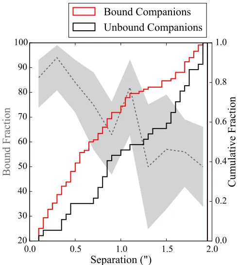
In Figure 10, we plot the bound fraction with confidence intervals, listed in Figure 9, in gray. We determine the 1σ confidence intervals for the bound fractions using the Clopper–Pearson binomial distribution confidence interval. This method is based on the full binomial distribution.

We also plot the cumulative distributions of the separations of bound and unbound stellar companions on the right axis(in red and black, respectively), showing distinctly different distributions in separation for these two populations. Approxi-mately 40% of close bound companions are located within 0 5 of their stellar primaries, and half of the detected bound companions are located interior to 0 7. On the other hand, the cumulative distribution places less than 50% of unbound companions interior to 1 2.

We perform a two-sample Kolmogorov–Smirnov test to determine whether the observed distributions of separations among the bound and unbound samples are consistent with being drawn from the same parent distribution. The null hypothesis that the two samples are drawn from the same parent distribution has a p-value of 0.002, indicating that the separation distribution for the bound companions is distinct from the distribution for unbound companions.

5. Planet Radius Corrections

Planetary radii for Kepler PCs are calculated assuming the planet resides in a single stellar system (e.g., Batalha et al. 2013; Burke et al. 2014; Mullally et al. 2015; Rowe et al.2015). For KOI hosts with stellar companions unresolved in Kepler photometry, however, the light from the stellar companion will dilute the transit signal, causing the planet to appear smaller than it actually is.

For the purposes of the planet radius correction analysis, we whittle our KOI host sample down to a relevant subset. Wefirst remove all KOIs with a disposition of FP, since these transit signals do not represent the presence of planets. We also remove several KOI systems with dispositions of PC, but planetary radii larger than 2RJ.

For confirmed planetary systems, we include only those systems without extensive and individual follow-up, including high-resolution imaging, available in the literature. For many of the confirmed systems in our sample, other research groups have discovered and accounted for the presence of a stellar companion in determining updated planet parameters. We do not repeat this analysis for these systems, since stellar multiplicity has already been addressed.

This subsample does not exclude all confirmed planetary systems, since 57 of 72 systems in our sample were confirmed without an explicit analysis of the effects of the stellar companion. Of these, eight achieved confirmed status by nature of their inclusion in multi-planet systems (Rowe et al. 2014). Five achieved confirmed status based on TTV analysis (Xie 2013, 2014; Van Eylen & Albrecht 2015). Morton et al. (2016) confirmed 45 systems statistically, but explicitly neglected the possibility that the planets might orbit a stellar companion. Since the planets in these 57 systems did not receive re-analysis including the full effects of the stellar companion, we must still account for the radius correction due

to the stellar companion. For these confirmed systems, and for the PC systems in our sample, we re-analyze the planetary radii to correct for the contamination of the transit signal by another star on the sameKepler pixel.

For stellar multiple systems, the ratio of the true planet radius to the assumed single radius can be estimated as

( )

( ) ( )

= =⎛

⎝

⎜ ⎞

⎠ ⎟

X R

R

R R

F F true

single 1

R p

p

t

t

1 tot

where Rt and Ft are the radius and the Kepler bandpass flux

from the transited star,Ftotis theKeplerbandpassflux from all

stars within the Kepler aperture, and R1 is the radius of the

assumed-single primary KOI star (Ciardi et al. 2015). This planet radius correction factor includes a component to correct for the dilution of the light from the stellar companion, as well as a component to correct for the assumption that the planet orbits the primary star, and thusR1is the relevant radius with

which to calculateRp. For any planets orbiting the KOI primary

star,

( )

= R

R 1 2

t

1

since the primary star is also the planet host(Ciardi et al.2015). Note that Equation (1) only provides an estimate of the radius correction factor for a given system. In order to more accurately assess the true planetary radii in a system with a close stellar companion, the original transit signal would need to be re-fit, in order to take limb-darkening and a potentially updated impact parameter into account. In addition, knowledge

of a stellar companion may change the interpretation of the primary star’s stellar properties, particularly for those stars with photometrically derived properties. These updates to stellar radius andTeff would also need to be addressed, on a

case-by-case basis, in order to fully correct the planetary properties. Without significant observational follow-up, we cannot fully assess which star in a stellar multiple system is the planet host. While an analysis of the position of the Kepler raw image centroids has been used in some cases to assess the location of the transit host star(e.g., Barclay et al.2015), for the majority of the systems in our sample, the stellar companion is too close and the centroid position too poorly constrained to rule out either the primary or the companion as the planet host. Additional modeling may make this technique for determining the planet host possible for the widest stellar companions and the largest planets in the sample, but it is beyond the scope of this work.

We therefore calculate XRn, the planet correction factor

assuming the planet host star is the nth component of the system, for each of our bound systems. In all cases but one, n=1 or 2, where the planets may orbit either the primary or bound companion. We report these values in Table 2. In the KOI 652 system, we detect two bound stellar companions, so we report XR3in the table comments.

For unbound or uncertain systems, we are unable to perform the same analysis, since we do not have a good estimate of the stellar parameters of the line-of-sight companions. Due to unknown interstellar extinction, we cannot assume that the colors we measure are representative of the intrinsic colors of these stars, and we therefore cannot rely on color–Teffrelations

to estimate these stars’radii. We only calculateXR1, based on

flux dilution, for these systems. However, it is still possible that the planets orbit the unrelated companion, rather than the KOI primary star. In this case, the planet radius correction factor may be significantly higher than theXR1value we provide. We

denote these systems in Table 2 with triple dots in the XR2

column.

Converting from units of flux to magnitudes, we write the ratio of true to assumed single planet radius as

( )

( ) ( )

( )

å

= =

=

- D -D

⎛ ⎝ ⎜ ⎞_⎠⎟⎛

⎝

⎜ ⎞

⎠ ⎟

X R

R

R R true

single 10 3

R p

p

t

n N

m m

1 1

2.5 1 2

n t

where Δmn is the ΔKp of the nth component and N is the

number of components in the system which fall on theKepler pixel, including the KOI primary star.Δmt is theΔKp of the

transited star, and Δmt=0.0 if the primary star is the

planet host.

Using the observedΔmvalues and colors of the companion stars, we calculate the degree of contamination due to the companion in the Kepler bandpass, ΔKp. For bound companions, we use the isochrone models to provide estimates of theΔmvalues in theKepler bandpass, using the weighted average of the absolute Kepler magnitude from each of the

“isochrone-shifted”models for the companion, as well as the absolute Kepler magnitude of the primary provided by the initial isochrone models.

For uncertain and unbound companions, we cannot use the isochrone models to accurately represent the stellar properties of the companion. Instead, we follow the conversions from the various measuredΔmvalues toΔKp described inF17. They take a weighted average among all available methods for each target, excluding the Kp−J and Kp−K color–magnitude estimates for targets with both J and K measurements. This provides an estimate of theΔKpfor each companion. We use this estimate for unbound and uncertain companions, whose isochrone models do not represent the background or fore-ground star observed.

We list the resultingΔKpvalues used for our analysis of the planet radius correction in columns(3)and (4) (if more than one companion lies within 2″of the primary star)of Table2. Three stars in our sample(KOI 975, KOI 3214, and KOI 5971) do not have the correctΔmmeasurements to calculateΔKpas described. These stars were measured withfilters for which we

Table 2

Radius Correction Factors

KOI Companions ΔKp21 ΔKp31 KOI Rp(Assumed RpReference XR1 XR2

within 2″ (mag) (mag) (Planet) Single) (Confirmed Planets)

5 2 0.29 3.01 5.01 7.07 1.352 2.239

5.02 0.66 1.352 2.239

105 1 3.75 105.01 3.05±0.43 Morton et al.(2016) 1.016 K

112 1 1.04 112.01 2.85±0.22 Morton et al.(2016) 1.176 K

112.02 1.25±0.1 Morton et al.(2016) 1.176 K

118 1 4.73 118.01 2.25±0.3 Morton et al.(2016) 1.006 K

119 1 0.29 119.01 8.65±0.48 Rowe et al.(2014) 1.330 1.347

119.02 8.18±0.51 Rowe et al.(2014) 1.330 1.347

120 1 2.96 120.01 31.09 1.032 K

Note.Radius corrections for planets and planet candidates in the stellar KOI sample. Column(1)indicates the KOI system. Column(2)gives the number of companions detected within 2″. Columns(3)and(4)provide theΔKpvalues for the secondary(ΔKp21)and tertiary companion(ΔKp31). Column(5)indicates the planetary candidate or confirmed planet. Column(6)gives the previous best estimate of the planet radius, either from theKeplerpipeline for planet candidates, or from the Exoplanet Archive(http://exoplanetarchive.ipac.caltech.edu/index.html) (with literature source in Column(7))for the confirmed planets. Columns(8)and(9) provide our calculated radius correction factors, assuming the planets orbit the primary(XR1)or secondary(XR2)star. In these columns, an indeterminate value

indicates a system in which we have too little information to calculate the radius correction factor because the system is uncertain or unbound, and we have no accurate estimate of the companion’s stellar radius.

Three target KOI hosts have more than two companions within 2″, which we include in the dilution correction analysis. These are KOI 387(ΔKp41=7.58 mag), KOI

2032(ΔKp41=0.32 mag), and KOI 3049(ΔKp41=7.48 mag,ΔKp51=4.92 mag).

Only one target, KOI 652, has two bound companions within 2″, allowing calculation ofXR3in this system. KOI 652 hasXR3=2.657.

do not have relationships that would convert the measuredΔm values toΔKp. KOI 975(Kepler-21)is analyzed in-depth and confirmed by Howell et al. (2012), who include analysis of high-resolution imaging data, so we do not re-analyze the planet radii in this system. For the other two systems without calculated ΔKp values, we cannot include a planet radius correction.

With knownΔKpvalues, we calculate the radius correction factors assuming the planet orbits the KOI primary star, XR1.

For bound companions we also calculate XR2, the radius

correction factors assuming the closest bound stellar compa-nion hosts the planets. The radius correction factors are listed in Table2.

Figure 11 shows the distributions of XR for the bound

systems, under four scenarios: in panel (a), we show the distribution of XR1, the dilution correction required to correct

planet radii if all planets orbit the primary KOI stars.

In panel (b), we use the relative occurrence rates of planets of various sizes to assess the relative likelihood that the larger or smaller stellar component hosts the planets (making the planets smaller or larger, respectively). We use the binned occurrence rates as a function of planet radius, marginalized over planet orbital period, from Howard et al. (2012). For a given planet, we calculate the radius assuming the planet orbits the primary star, and the larger radius assuming the planet orbits the secondary. We then compare the relative occurrence rates at these two planet radii, and weight our XR average by

these occurrence values.

The relative occurrence rates used for this analysis are marginalized across orbital period and stellar mass. This process is further complicated by a lack of understanding of the occurrence rates of planets in binary star systems, which may be very different from planets in single-star systems. However, this simple analysis allows us to leverage previously measured planet occurrence statistics and improve our estimate of the possible planet radius corrections.

In panel(c), we assume the planets are equally likely to orbit the primary and secondary star, and take a simple average of theXR1andXR2values. In panel(d), we show the distribution of

XR2, the radius correction factors needed if all planets orbit the

smaller secondary stars.

For KOI 652, which has two bound stellar companions within 2″, we only include XR2 in the plot. However, we

provide an estimate ofXR3in the comments of Table 2.

Under the assumption that planets in bound stellar multiple systems are equally likely to orbit either the primary or secondary star, a mean radius correction factor ofXR =1.65is

found, indicating that planets in binary systems may have radii underestimated, on average, by 65%. The weighted average scenario may be more realistic, and provides a mean radius correction factor ofXR=1.44.

Ciardi et al.(2015) predict that the average radius correction factor for the Kepler field should beá ñ =XR 1.6 for G dwarfs

without radial velocity and high-resolution imaging vetting of KOI host stars. They assume the multiplicity of theKeplerfield is comparable to the solar neighborhood(Raghavan et al.2010), and that planets are equally likely to orbit any component of a stellar multiple system. Comparable multiplicity to the solar neighbor-hood was shown to be a reasonable assumption by Horch et al. (2014)based on high-resolution imaging, which is most sensitive to stellar companions at fairly large physical separations. However, there are indications that multiplicity may be suppressed at smaller separations (e.g., Wang et al. 2014a, 2014b; Kraus et al.2016), and other effects such as Malmquist bias may also play a role in determining what fraction ofKepler planet hosts have unknown stellar companions.

We would expect that our average measured XRfor bound

systems in our sample should be greater than the predictedá ñXR for the full Kepler field, since we do not include any single stars (XR=1.0) in our analysis. If we make the simple

approximation that our detected bound binary systems are representative of all binary systems in theKeplerfield(i.e., all Kepler field binaries have a mean radius correction factor of

=

XR 1.65, like our sample binaries), and assume that 46% of

allKeplerstars are binaries(as the multiplicity statistics of the solar neighborhood indicate), then we would expect a mean radius correction factor for the full Kepler field of XR =1.3,

smaller, but roughly consistent with the predictions of Ciardi et al. (2015). Note that this simplistic analysis neglects unassociated background stars entirely, and a more complete analysis would also account for the variation in typical binary mass ratio(orΔm)as a function of separation.

Figure 11.Distribution of planet correction factors,XR, for the bound systems in our sample. These include the dilution factor as well as correcting for the radius of the

transited star. Panel(a): all planets assumed to orbit the primary KOI;XR=XR1. Panel(b):XRcalculated by weighted average, based on the relative occurrence rates

of planets of various sizes. Panel(c): planets equally likely to orbit primary or secondary star;XR= á ñ =XR 0.5(XR1+XR2). Panel(d): all planets assumed to orbit

In Figure12, we plot the distribution of planet radii for KOIs in our sample, divided into specific, uneven bins corresponding to planet type: <1.25RÅ for Earth-sized planets; 1.25–2.0RÅ

for Super-Earth-sized planets; 2.0–6.0 RÅ for Neptune-sized

planets; 6.0–15.0RÅ for Jupiter-sized planets; and >15.0RÅ

for planets larger than Jupiter. In gray, we plot the number of planets in our sample in each of these bins, prior to radius correction. In color, we plot the distribution of corrected radii under the same four scenarios as in Figure 11, but including unbound and uncertain stellar systems as well as bound systems. In all cases, we only apply the dilution correction,XR1,

to unbound and uncertain systems.

Figure12clearly shows that dividing planets into bins based on uncorrected planet radii can cause significant overestimates of the occurrence of small planets; in all four scenarios, the population of Earth-sized and Super-Earth-sized planets in our sample decreases significantly when radii are corrected for the presence of stellar companions, while the number of Neptune-sized and Jupiter-Neptune-sized planets increases. The amount by which the population sizes change depends upon assumptions about which star hosts the planets. This type of analysis, performed by Ciardi et al. (2015) on a synthetic Kepler population, predicts that the occurrence of small planets(<1.6RÅ)may be

overestimated by 16% unless stellar multiplicity is accounted for.

It is important to note that there is a corresponding effect acting in the opposite direction, potentially causing the occurrence of small planets to be underestimated. Specifically, the increased difficulty offinding small planets in systems with stellar companions means our sensitivity to small planets may have been overestimated. In truth, we are likely missing many small planets whose transits are heavily diluted by a stellar companion.

The relative scale of these two effects is difficult to quantify and is beyond the scope of this paper to calculate. However, we provide an estimate of the minimum detectable planet size for a

typical binary system in our sample. KOI-1830 has an apparently bound stellar companion separated by 0 46 from the primary KOI star, with a ΔKp=2.65±0.08 mag, the median value of ΔKp in our sample. KOI-1830 hosts two planets which were statistically validated by Morton et al. (2016), although the validation did not fully account for the stellar multiplicity. Prior to the discovery of the stellar companions, the best estimates of the planetary radii were 2.35±0.1 and 3.65±0.15RÅ, with transit depths of 823 ppm and 2060 ppm. The orbital periods of the two planets are 13.2 and 198.7 days. Based upon our work, wefind that the planets are underestimated by a factor ofXR1=1.042(planets orbit the

primary)or XR2=2.409(planets orbit the secondary).

Based on the reported transit depths and S/N values, we estimate how small each of these planets could be before it became undetectable around each of the stellar components. S/N depends linearly on transit depth as:

( )

d s

= n t

S N

3 hr 4

CDPP tr dur

/

(Howard et al.2012).

We define a minimum transit detection threshold(δthreshold)

such that the minimal signal-to-noise of a detected transit must be …7.1 (as is the case for the Kepler pipeline). For the two transiting planets (at their respective orbital periods), the minimum detectable transit depths areδthreshold=119 ppm and

346 ppm, respectively. Assuming no dilution by a stellar companion, these depths correspond to planetary radii of 0.89RÅand 1.5RÅ. However, taking into account the presence

of the stellar companion, the minimum detectable planet sizes are 0.93RÅ and 1.56RÅ, if the prospective planets orbit the

primary star, and 2.15RÅand 3.6RÅ, if the prospective planets

orbit the secondary star.

Thus, while we might assume the data are sensitive to all planets in KOI-1830 that are larger than 1.5RÅwith an orbital period of 198.7 days, planets as large as 3.6RÅmight actually

Figure 12.Distributions of originalKeplerpipeline and updated planet radii for all planet candidates and confirmed planets without high-resolution imaging analysis in our sample. We divide the KOIs in our sample into bins representing planets of different types: Earth-sized planets (<1.25RÅ), Super-Earth-sized planets

be present without being detected. Likewise, planets with sizes of 0.89–2.15RÅ might be undetectable at orbital periods of 13.2 days.

The true frequency rates, and associated uncertainties, of planets as a function of planetary size must take into account the probabilities that the stellar systems contain more than one star. Future efforts in this direction might allow us to assess the combined impacts of stellar multiplicity on planet occurrence statistics.

6. Conclusions

High-resolution imaging follow-up is essential for accurate estimation of transiting planet radii. It will prove especially useful for planets discovered by theK2andTESSmissions, due to their inclusion of closer, brighter stars than theKeplerprime mission. If stellar companions (both bound companions and chance line-of-sight background stars)cause significant underestima-tion of the Keplerplanet radii, this will certainly compromise calculations of planet occurrence, which divide the ensemble planet population into bins in planet size. Additionally, studies of the boundary between rocky and gas giant planets rely on comparing planet densities in bins of planet size. If both the densities and radii of planets are inaccurate due to a stellar companion, conclusions about the nature of small planets may beflawed.

We find that Kepler planets in binary systems have radii underestimated by a mean radius correction factor of

á ñ =XR 1.65, meaning their radii are underestimated, on

average, by more than 50%, assuming an equal likelihood of orbiting either component (á ñ =XR 1.44if weighted by planet

occurrence rates at different planet sizes). Expanding this to the full Kepler sample, including single stars, we predict that the average radius correction factor for the fullKeplerfield should be 1.3, roughly consistent with the simulation results from Ciardi et al.(2015).

We confirm that very close stellar companions are highly likely to be bound, as predicted by Horch et al. (2014). We show that if a companion is detected within 2″, the star is likely bound (50%), and if detected within 1″, the star is almost certainly bound(80%).

Finally, we provide a demonstration of how uncorrected planet radii might bias a radius-based study of planet occurrence. For our sample, wefind that correcting for stellar multiplicity or line-of-sight stellar companions significantly decreases the number of Earth-sized and Super-Earth-sized planets, while increasing the number of Neptune- and Jupiter-sized planets in the sample. We also demonstrate the effect of stellar dilution making small planets that might otherwise be counted among Earth- and Super-Earth-sized bins effectively undetectable, thus biasing small planet occurrence in the other direction.

The specific amount by which multiplicity biases the sample sizes of different types of planets depends heavily on assumptions about the multiplicity of the stars in the sample, as well as assumptions about which stars in a stellar multiple system host the planets. The best way to account for this problem is by using high-resolution imaging follow-up to rule out stellar companions whenever possible. This technique will be even more effective for the upcomingTESSandK2samples, which have much smaller average stellar distances than the Kepler sample.

Although we do not perform a full statistical analysis of the multiplicity of the Kepler planet hosts to assess how multi-plicity affects planet formation and evolution in this work, we do provide a new sample of Kepler planets in bound stellar multiple systems for this type of work in the future. A full analysis of the bias inherent in the selection of our sample would be required in order to make any statements about this subject.

We thank the anonymous referee for a thorough and detailed report and many helpful suggestions and comments. This project was begun during and partially funded by the Infrared Processing and Analysis Center’s Visiting Graduate Student Fellowship at the California Institute of Technology. The authors would like to thank James Graham for useful discussions while working on this project. This research has made use of the NASA Exoplanet Archive and ExoFOP, which are operated by the California Institute of Technology, under contract with the National Aeronautics and Space Administra-tion under the Exoplanet ExploraAdministra-tion Program.

Software: Dartmouth Stellar Evolution models (Dotter et al.2008), TRILEGAL (Girardi et al. 2005).

Appendix

Notes from Table1

(a)Additional companion to KOI 5 detected in the K-band by Kraus et al. (2016) at 0 03, but no color information is available to perform physical association assessment.

(b) Two additional companions detected around KOI 68; both are separated by more than 2″, so are not included in the sample. KOI 68 C is located at 2 74 and appears to be unbound. KOI 68 D is located at 3 41 and appears to be bound.

(c)Additional companion to KOI 105 detected at 3 88 has uncertain designation.

(d)Three additional companions are detected near KOI 113. KOI 113 C was detected in theK-band at 1 32 by Kraus et al. (2016), but no color information is available. Two additional companions at 3 21 and 3 63 are outside the separation limit of our sample. KOI 113 D appears bound, while KOI 113 E appears unbound.

(e)Two additional companions are detected near KOI 177, at 2 29 and 2 87 respectively. Neither of these companions has available color information.

(f)Additional companion to KOI 227 detected at 3 35 in K-band, but no color information available.

(g) Additional companion to KOI 268 detected at 2 51 appears to be unbound.

(h) Additional companion to KOI 285 detected at 2 33 appears to be bound.

(i)Additional companion to KOI 298 detected at 2 01 in i-band by AstraLux, but no color information is available.

(j) Additional companion to KOI 378 detected at 2 91 appears to be bound.