I. Numerical solution of exact pair equations. II. Numerical solution of first-order pair equations

I.

NUMERICAL SOLUTION 0 F EXACT PAIR EQUATIONS

II. NUMERICAL,

SOLUTION OF FffiST-ORDER PAIR EQUATIONS

Thesis by

Nicholas Wilhelm Winter

In Partial Fulfillirent of the

Requirements

For the

Degree of

Doctor of

Philosophy

California Institute of Technology

Pasadena, California

1970

ii

ACKNOWLED GMEN'TS

I would like to thank my research advisor, Dr. Vincent Mc Koy,

for his encouragement during my graduate study. I am also indebted

to Dr. William A. Goddard for many discussions and helpful advice.

The first three years at Caltech were enriched by

rrrf

interactions with

Dr. Russell M.

Pitzer.

Perhaps I learned the most from my contacts with other graduate

students. I am particularly grateful to Dr. Thomas H. Dunning for

the many projects on which we collaborated. I am also thankful for

the many discussions with Donald Truhlar and Luis

Kahn.

Finally, the most important contribution to my graduate study

has been from my wife, Barbara Jo. Her patience and understanding

iii

APSTRACT

Part I

Numerical solutions

to the

S-limit equations for

the

helium ground

state and excited

triplet

state

and the

hydride

ion ground

state are

ob-tained with the second

and fourth

difference approximations. The

results for the ground states

are

superior to previously reported

The coupled equations resulting from the partial wave expansion of

the

exact helium atom wavefunction were solved giving accurate S-, P-, D-, F -,

and G-limits. The G-limit is -2. 90351 a. u. compared

to

the exact

value of the energy of -2

.

90372

a. u.

Part

II

The

pair

functions

which

determine the exact first-order

wave-function for

the

ground state of

the three-electron atom

are found

with

the matrix finite

difference method.

The second-

and third-order

energies for the (lsls)

S,

(ls2s)

S, and (ls2s)

S

states of

the

two-electron atom

are presented

along with contour and perspective

plots

of the

pair functions

.

The

total

energy

for the

three-electron atom

with a nuclear charge Z is found

to

be

iv

TABLE OF CONTENTS

PART

TITLE

PAGE

I

NUMERICAL SOLUTION OF EXACT PAffi

EQUATIONS

A. Introduction

1

B. Partial Wave Reduction of the Two-Electron

Equations

5

c.

Review of the Finite Difference Method

7

D. Solution of the S-Limit Equation

10

E

.

Solution of the Coupled Partial Wave Equations

for the Helium Atom

16

F

.

Discussion

19

REFERENCES

20

TABLES

22

F1GURES

35

II

NUMERICAL SOLUTION OF FIRST-ORDER PAffi

EQUATIONS

A. Introduction

43

B. Reduction of the First-Order Equation

44

c.

Solution of the First-Or

d

er Pair Equation

49

D. Calculation of the Seco

nd

- and Third-Order

Energies for the Two-Electron States

52

E. Contour and Perspective Plots of the Pair

v

PART

TITLE

PAGE

F

.

Calculation of E

and

for the

Three-Electron Atom

59

G. Discussion

63

·

REFERENCES

64

TABLES

66

F1GURES

78

1

It

is a well established approach to the study of electron

correlation to analyze the many-electron system as a series of

simpler two-electron problems. Sinanoglu

1

has shown how the

first-order equation can be reduced to two-electron pair equations

for the many-electron atom or molecule. He also discusses the

equation for "exact pairs" which describes the pair correlations

beyond first-order. N esbet

2

has been successful in reducing the

total wavefunction and energy for first-row atoms into their

Hartree-Fock and two-body components. The general topic of electron

cor-relation is reviewed

in

Refs. 3 and 4.

We are not concerned here with the derivation_

or validity

of the various pair approximations but with how to accurately and

efficiently solve the resulting equations. There have been tv.;o

stan-dard approaches in the past, both of which are variational. The

first dates back to the early calculations of Hylleraas

5

who used a

trial function containing inter electronic coordinates. The unspecified

parameters are determined so as to minimize the two-electron

energy. This method is capable of high accuracy

if

enough terms

are included, but leads to difficult integrals to evaluate. Indeed

considerable research effort has gone into the study of these integrals

themselves. The most successful approach is to use a configuration

2

in part to its general applicability.

When applied

to

the

pair equations'\

the CI method obtains the pair energies and

properties

without dealing

directly

with

a two-electron equation. Instead

the total N-electron

.

wavefunction is constructed from a set of Slater determinants so

as

to describe the correlation between a specific pair of electrons

while

treating the remaining N-2 electrons in

the

Hartree-Fock

approxima-tion. The energy is found by diagonalizing the total Hamiltonian

in

this basis. This

is

equivalent

to

solving a Schrodinger equation

des-cribing the pair of electrons correlating in the Hartree-Fock field

of the remaining N-2 electrons. The principal disadvantage of

the

CI method is the slow convergence relative to the use of

interelectronic

coordinates. Schwartz

61

7

has pointed out the disadvantages of using

orbital expansions to represent correlated wavefunctions

with

parti-cular attention to the convergence as higher angular configurations

are included.

We have chosen

an alternative to

these approaches by simply

solving the equations numerically. Since it

is

not possible to

treat

a six-dimensional equation,

we

first

eliminate the

angular

variables

by

a partial

wave expansion.

Then

the resulting equations for

the

functional coefficients are solved numerically. The method

is not

variational and does not necessarily

give an upper

bound

to the

two-electron energy. However, once

the

basic

techniques are established'\

3

This allows one to consider a variety of approximations to the pair

·

equations (pseudo-potentials, etc.) without additional complications.

The numerical methods are highly computer oriented,since the

dif-ferential equation is reduced to a set of difference equations which

are solved by standard matrix techniques.

In

two earlier papers

8

'

9

we applied the matrix finite difference

.

(MFD)

method to the solution of the S-limit Schrodinger equation and

the first-order pair equation for the helium atom. The results were

accurate; however, in order to apply the method to excited states

of two-electron atoms and to the valence electron pairs in first-row

atoms,

it

was necessary to reexamine the numerical techniques.

The most obvious problem originates from the diffuse nature of the

wavefunction describing these electron pairs. This requires that

the point at which the solution is required to vanish must be taken

further out and consequently the number of points needed to obtain

an accurate solution becomes unreasonable. Another refinement is

needed when considering the solution of exact pair equations. The

partial wave expansion qf the exact pair function leads to a set of

coupled equations in contrast to the first-order pairs which give

uncoupled equations

.

The exact pair functions are solutions of

eigen-value equations differing from the two-electron atom Schrodinger

equation only in the presence of the potential due to the N-2 "core"

4

have to iterate among the equations determining the functional

co-efficients of the partial wave expansion. To keep the problem within

limits we must be able to obtain accurate solutions with a small

number of points.

I

We have corrected for the possible diffuse nature of the pair

functions by transforming to a new set of variables which are just

the square roots of the original variables.

In

order to guarantee

greater accuracy with fewer points

,

fourth differences have been

in-cluded in the approximation of the derivatives. Combining both of

these modifications with an extrapolation procedure, we have found

the S-limits for the ground states of helium and the hydride ion. The

equations were also solved using both transformed and untransformed

coordinates and second differences only. With the three sets of results

for each atom, we can compare the effectiveness of the modifications

for a tightly bound pair (helium) and a diffuse pair (hydride ion)

.

Finally, we have applied the MFD method to the exact Schrodinger

equation for the helium atom using successively higher partial waves

up to the G-

linit. The results proved superior to any previous CI

calculation of the angular limits. The properties predicted by the

5

B. PARTIAL W

A

VE REDUCTION OF THE TWO-ELECTRON E

The partial wave expansion of the solution of the two-electron

SchrOdinger equation has previously been considered by Luke, Meyerott,

and Clendenin

10

for the

S state of Li+

.

For a spherically symmetric

pair of electrons the exact wavefunction can be expanded in Legendre

polynomials of the cosine of the relative angle between the two

elec-trans,

Cf)

'li'(r1r2812)

=

L

.e

=0

By substituting this into the equation,

(1)

(2)

multiplying both sides by

~

P

1

(cos

8

and integrating over all

angular variables

we obtain the

Q

-th member of an infinite set of

6

[-t

(l/r~

a/ar, (r: a/ar,) +

1/r~

a

/

ar.

(r~

a/ar.))

+

f

(t+ii;2r: +

f(f+l)/2r~

+

V(r

+ V(r

+

MH

J

!Jlf(r

r

where

and

k

C (Qo,

lo)

MQQ'

=

=

../(2Q

+

1)(2Q'+ 1)

2

'

(3)

Up to this

point we

have

not made

any approximations,

although

it

is clearly an impossible task to solve an infinite set of coupled equations.

7

to the desired accuracy. When using the MFD method it is convenient,

but not necessary, to begin by solving the S-limit (

=

0 partial waye

only) and then use this as an initial guess to determine the P-limit

(

Q

=

0, 1

partial waves only) and so forth. After two partial waves

,

the addition of further terms to the expansion has a small effect on

the lmown functional coefficients and the iterative method of solving

the coupled equations converges extremely rapidly. Therefore

,

the

slow convergence of the partial wave expansion pointed out by Schwartz

7

is not a serious drawback.

It

is easy

to

show that a similar reduction of the Schrodinger

equation can be made for pairs that are not spherically symmetric

.

The main difference appears in the angular integrals which couple

the equations together. Also

the non-local potentials which occur in

the Hartree-Fock pair equations offer little complication since the

equations already contain nonhomogeneous term>. The numer

ical

techniques needed to solve these equations are presented in the next

section

.

The second derivative can be expanded in terms of differences

8

where

6~

=

tJ;(r

+

h) - 2tJ;(r

+

tJ;(r

h)

6~

=

tJ;(r

+

2h) - 4tJ;(r

+

h)

+

6tJ;(r

4tJ;(r

h)

+

tJ;(r

2h)

o~

=

tJ;(ro

+

3h) - 6tJ;(ro

+

2h)

+

15tJ;(ro

+

h) - 20tJ;(ro)

+

l 5tJ;(r

h) - 6tJ;(r

2h)

+

tJ;(r

3h)

(5)

and h is the grid size.

11

The first approxi:tra.tion to the second

derivative is just a

tj;/ar

1/

h

6

In

order to find the difference

error we expand the second difference in terms of derivatives

=

( 2

a

VI

I

a

r

2)

2( 4

I

4)

4( 6

I

6)

0

+

12 • h

a

1/J

a

r

+

h

a

VI

a

r

+

•

..

(6)

and as a consequence of choosing central differences, the error

contains only even powers of h. Bolton and Scoins

12

have shown

that the energy found with a grid size h can be expressed as a power

series of the form

E(h)

(7)

where E(O) is the exact energy corresponding to h

=

0. For most

two-dimensional equations it is not possible to use enough points to

9

used to extrapolate the energies found at several grid sizes to the

exact value.

13

Fox

14

has argued that a substantial amount of the difference

·

error can be eliminated by including the next term in the difference

expansion of the derivative in the MFD equations. The difficulty in

using fourth differences is satisfying the boundary conditions. The

usual conditions are to require r

·

t/;(r) to vanish at r

=

0 and r

=

r

max

where r max approximates infinity. The fourth difference of t/;(r)

·

at

r

=

h requires that we know the function at r

=

-h, and therefore

introduces uncertainties into the MFD equations. A similar difficulty

occurs at the other boundary. One solution of this problem is to

extract the asymtotic behavior of t/;(r) at r

=

0 and r

=

from the

differential equation and use this to relate the unknown values of t/;(r)

-outside the defined grid to the values within. This is the approach

we have taken for the fir st-order pair equations; however, for

.

the

eigenvalue equations, it is simpler to replace the fourth difference

approximation at the boundary with the usual second difference

ap-proximation. This does not appreciably affect the accuracy when

combined with the coordinate transformation to be discussed later.

Unfortunately, the fourth difference approximation does not

sufficiently reduce the difference error to be used without

extrapola-tion. The approximation does allow accurate results to be obtained

10

for the S-limit equation in the next section.

Truncating the partial wave expansion at

1

=

0, we then obtain

the following equation for the two-electron atom,

where u

(r

r

=

r

r

lf;

(r

r:,i).

If

the derivatives are replaced by the

second difference approximation, (8) is transformed to a set of linear

equations of the form,

D·u

=

E·u

(9)

where

D

is a symmetric banded matrix with non-zero off-diagonal

elements in only two super-diagonals and two sub-diagonals. The

eigenvectors at

D

represent the ground and excited states of the

two-electron equation and would be exact if we used an infinite number

of grid points and satisfied the correct boundary conditions

.

Since

we are usually satisfied with the lowest state and possibly a few

excited states, a finite number of points are enployed and a

11

We have solved the S-limit equation for the first two states

of

the helium atom and for the ground state of

the hydride ion using

the second difference approximation. The radial cutoff for the ground

state of helium was taken at 9 a. u. and for the excited state at 20 a. u.

For the hydride ion the solution was required to vanish at 25 a

.

u.

Equation (8) was solved for several grid sizes and the eigenvalues

extrapolated using the polynomial representation of the difference

error. From (7) we see that two eigenvalues are needed to eliminate

the h

-term, three for the h

and h

-terms,

etc.

We have done this

for the three states and present the results in Tables I-III.

The extrapolation of the S-limit for the helium ground state

predicts an energy of -2. 879031 a. u. with an uncertainty in the last

figure. The previous best limit was found by Davis

15

and by Schwartz 7

to

be

-2. 879028 a. u.

Table I

shows

the extrapolated values found

-'

using successively more of the initial energies to be converging from

above. Thus the best extrapolant should be an upper bound to

the

true S-limit. This value falls within

the

error bounds on Davis'

predicted limit

.

s

.

The results for the S state of helium and the ground state

of the hydride ion are less satisfactory. Davis

15

'

16

places the

S-limits

of these

states at -2. 1742652 a. u. and -0. 5144940 a. u. ,

respectively. The

MFD

method is more difficult for these states

12

we have, it was necessary to diagonalize a matrix as large as 22, 500

by 22, 5000 for the

S state and about 15, 000 by 15, 000 for the hydride

ion.

In

order

to

avoid this problem, we made the following

co-ordinate tr ans formation,

2

=

"2

(10)

and solved the Schrodinger equation on an evenly spaced grid in x

and Xa· The effect of this is to give a dense distribution of points

near the nucleus and a sparse distribution in the tail regions

,

as

viewed in the untransformed system

.

Not only is the radial cutoff

less important in the new system, but since this is a more optimum

distribution of points for our problem, we can use fewer points

with-out losing accuracy

.

Substituting the transformation into (3), the derivatives

become,

1/r

a

/

ar(r

a/ar)

=

1

/

4r (a

/

ax

1

/

x a

/

ax)

(11)

13

which leads to the following equation for

1

(12)

This equation was solved for the hydride ion with a 25 a. u. radial

cutoff (5 a. u. on the square root grid) using grids ranging from 25

to 50 strips. The results extrapolated to E

=

-0. 514497 a. u. and

were converging from below. Representation of the difference

error using only even powers of h was not as efficient for the new

coordinates giving an energy of -0. 514557 a. u. , also converging

from below. Therefore a polynomial containing both even and odd

.

powers, but leading off with h

was used. The square root grid

reduced the computation time by a factor of 7 for this case.

In

an effort to improve the MFD method further, the

four

th

difference approximation was used

to

re-solve the equations for

helium and the hydride ion on the square root grid. The cutoff for

helium was kept at 9 a. u. but the cutoff for the hydride ion was

taken at 30 a. u. The energies obtained using both second and fourth

difference approximations are given in Table IV. While the fourth

difference results are improved, the accuracy is not sufficient to be

used without extrapolation.

In

order to

find the

appropriate

14

the grid size using successively finer grids. By studying the trends

in the extrapolants and the coefficients of the power series, we can

determine the most efficient form to represent the difference error.

The results for the polynomial fits of the helium energies are given

in Table

V.

The best representation of the difference error for the second

difference approximation is given by the polynomial containing a

cubic term in h. For the fourth difference results the polynomial

E(h)

(13)

appears to give the best extrapolant, but by eliminating odd powers

entirely we obtain accurate results and uniform convergence from

above. We should point out that while the error in the fourth

differ-ence approximation leads off as h

using second differences at the

boundary introduces the h

term

.

Table V1 gives the equivalent

information for the hydride ion. The fourth difference approximation

predicts an S-limit energy of -0. 514491

0. 000001 a. u. which is

within the error bounds of Davis' result

.

Even though the wavefunctions found by the MFD method are

only known at discrete points, there is no problem extracting the

same information from them that a variational solution can yield.

In

fact, the numerical solutions are generally of a higher quality

15

illustrated by the local energy which agrees with the eigenvalue to

six or more decimal places at every grid point. Properties are

easily calculated by quad!'ature methods which amount to nothing

more than double summations. These are then extrapolated in the

same manner as the ener

g

y.

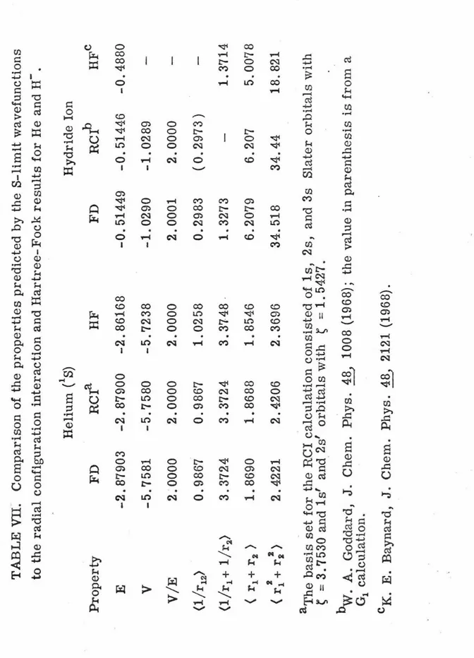
We have calculated sever

a

l properties from the fourth

dif-ference S-limit functions for helium and the hydride ion and compare

them to the radial CI and Hartree-Fock values in Table VII. The

agreement is

v

,

~ry

good except for

(r~

+

r~),

which indicates that

more diffuse basis functions were needed

·

in the radial CI calculations.

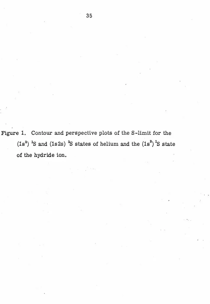
Contour and perspective plots of the two helium states and the

hydride ion ground state are given in Fig.

1.

We have plotted the

square of the function u

(r

r

in each case. The contour plots show

the regions rllr

~

4. 5 a. u. for the

S state of helium, r

r

~

10 a. u.

for the

3s

state, and r

r

12

.

5 a. u

.

for the hydride ion. The

nucleus is positioned at the lower left corner and the constan

t

contour

increment is given in the upper right corner. The lowest contour is

labeled

.

In

the 3-D plots the regions shown are r

r

7. 5 a. u

.

for

the helium

1s

state, r

r

~

13

.

3 a. u

.

for the

S state, and r

r

~

18

.

7 a

.

u

.

for the hydride

.

ion. F

i

gure 2 gives the viewer's orienta

-tion for these plots

.

The functional axis has the same scale

in

each

case so that the heights of the surfaces can be compared. The

16

the line r

=

r

The helium atom shows a similar feature for large

radial distances but only slightly. This minimum is not present for

the Hartree-Fock wavefunction which does not predict a stable ground

state for the ion.

While including radial correlation relative to the Hartree-Fock

model leads to a stable ion, the S-limit functions gives unreasonable

values for some properties. The exact value of

(r~

+

r~)

is 23

.

827

a. u. ,

17

which is about two-thirds of the S-limit value.

If

we include

the higher partial waves in our expansion of the exact solution, the

S-wave contracts and the expectation values approach the exact

re-sults. This is illustrated for the helium atom in the next section.

E. SOLUTION OF THE COUPLED PARTIAL WAVE EQUATIONS

FOR THE HELIUM

ATOM

The MFO method was applied to the sets of coupled equations

that result when

(1)

is truncated at

i

=

1,

2, 3, and 4

.

We decided to

use the second difference approximation on the linear grid with a

9 a. u

.

cutoff since this proved to be very accurate for the S-limit.

For a more diffuse state the square root grid would have been used.

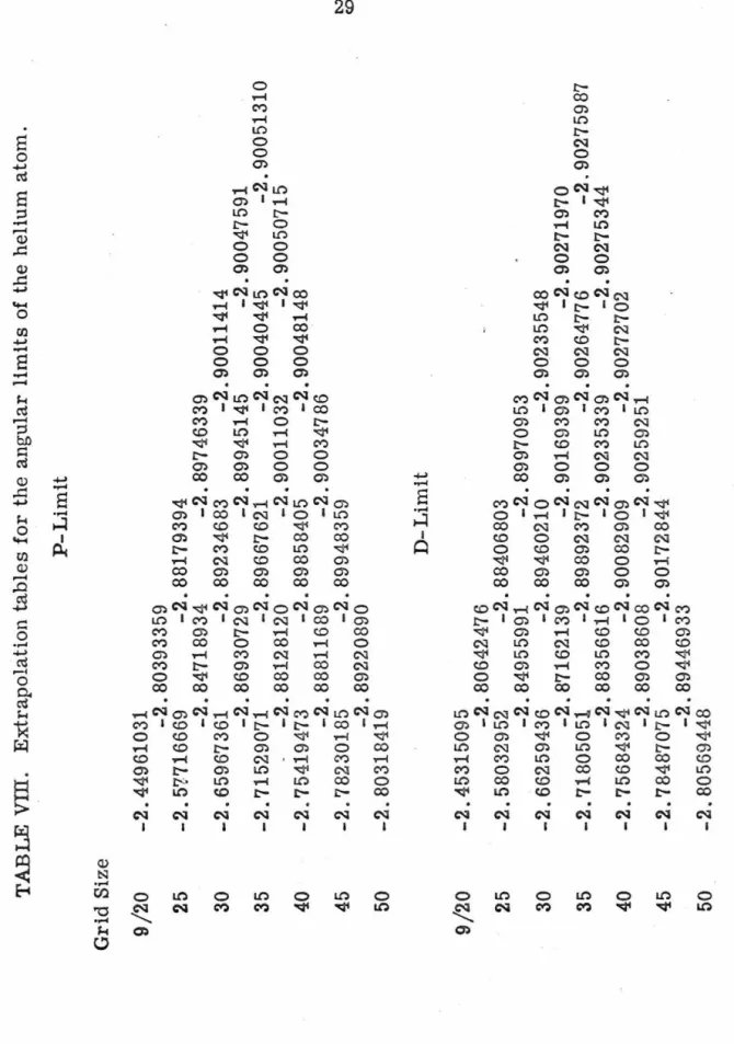
The extrapolation tables for the angular limits are given in

Table VIII. The results converge from above so that the best

ex-trapolants

should be upper bounds to the true limit. These are com-

.

17

numerical G-limit is superior

to

each of the other calculations.

Tycko, Thomas, and King

18

were only able to obtain an energy of

-2. 90344 a. u. using 15 partial waves. This illustrates the difficulty

in representing the functional coefficients with orbital products for

the higher partial waves.

·

As pointed out by Schwartz, 7 this led to

the erroneous conclusion that the majority of the error was in the

S-limit and that the contribution from the higher waves could be

neg-lected. The CI calculations

generally

do worse for the higher angular

limits, because to keep the calculations

from

becoming intractable,

fewer configurations are used to represent the

functional

coefficients.

The 11FD method

a:ctually

becomes easier for these equations since

the coefficients have less and less amplitude and are concentrated

nearer the line r

=

r

The energy can be expressed in the form,

(14)

where

=

18

Using the G-limit solution,

we

have calculated

the

different terms

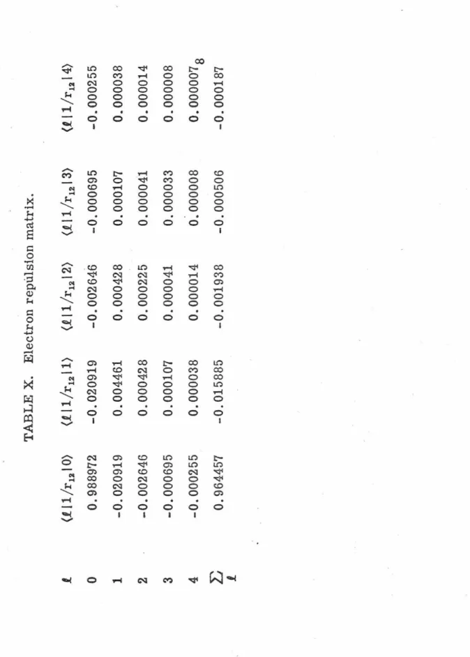
in this expression. The electron repulsion matrix elements

L

(.P..

I

r

<

k

I

r>

k+l

I

P..')

.

C

k (

P..o, P..'o

)

are presented m Table X and

.

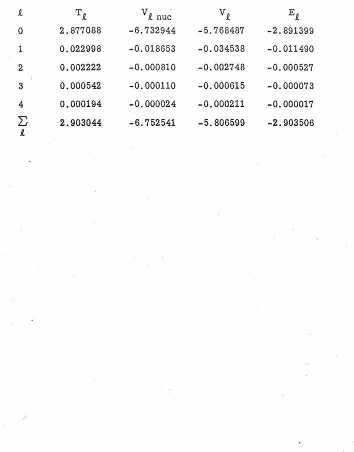
k

the energy analysis in Table XI. These results illustrate the small

but important effects the higher partial waves have on the energy.

Several properties were studied in the same manner and compared

to the exact values in Table XII. The accuracy is very good, being

about four decimal places in every case except for

(r~

+

r~)

. The

value is still too large and would improve

if

more partial waves

were

used.

The contour plots of each functional coefficient for the G-limit

are given in Fig.

3.

Again

the squares of the functions u

2

(r

r

are

plotted over the region r

r

4. 5 a. u

.

.

The

peakedness

of the higher

partial

waves

about the line r

=

r

is quite evident. Since

the

am-plitude of the functions for

>

0 is negative, their effect is to reduce

the

electron density in

this

region. Figure

4

gives

the

perspective

·

plots of

the

S- and P-waves using

the

same

scale along the fu...11ctiona.l

axis.

By integrating over

the

radial

variables, we found

the

volume

under the P-wave surface to

be

0.

4

%

of

that

under

the

S-wave. The

remaining waves

were too

small

to be

shown

with this

scale, but

the same integration showed the D-wave to be 5% of the P-wave and

19

F. DISCUSSION

~

The results presented here demonstrate that the numerical

solution of partial differential equations can

give

accuracy competitive

with variational methods. The values found for the S-limits of

helium and the hydride ion are superior

to

any previous calcuiation

and agree well with the predicted limits given by Davis.

More

im-I

i •

portantly

the

same accuracy was found when the coupled equations

were solved for helium. The equations describing

the

pair

correla-tions in atoms offer virtually no new consideracorrela-tions once

they

are

derived. The same program which was used for

the

helium atom

has been used to calculate the valence pair correlation energy for

beryllium and the

MFD

method has been applied

to

the first-order

hydrogenic pair equations for lithium. The results were consistently

accurate in all cases.

The calculations reported here

were

carried out on the CDC

6600

and IBM 360-75 computers. The IBM 360-75 results

were

found using

20

REFERENCES

~

*

This work is based on a thesis submitted by

N.

W. Winter

in partial fulfillment of the requirements for the degree of

·

Doctor

of Philosophy in Chemistry, California

Institute

of Technology.

t

Present address: Battelle Memorial Laboratory, Columbus,

Ohio.

·i-"'Present address

:

Chemistry Department, Rhode Island

College, Providence, Rhode

§Contribution No.

1

o

.

Sinanoglu, J. Chem. Phys. 36, 3198 (1962).

2

R. K. Nesbet, Phys. Rev. 175, 2 (1968).

3

o.

Sinanoglu

,

Advan.

Chem. Phys.&, 315 (1964).

4

R.

K.

Nesbet,

ibid.~'

321 (1965).

5

E.

A.

Hylleraas

,

Z. Phyzik 54, 347 (1929)

.

6

c.

Schwartz,

Methods

in

Comp

.

Phys.

1,

241 (1963).

7

c.

Schwartz, Phys. Rev

.

126,

1015 (1962)

.

8

N. W. Winter

,

D. Diestler, and

V.

McKoy,

J.

Chem. Phys.

48,

1879 (1968).

9

v.

Mc

Koy

and N.

W

.

Winter,

ibid.

4

8, 5514 (1968)

.

10

P

.

Luke

,

R.

Meyerott

,

and

W.

Clendenin, Phys. Rev.

85,

401 (1952)

.

11

The grid

size is given

by

h

=

r n/n-1 where

r n is the

last

21

12

H. C. Bolton and H.

I.

Scoins, Proc. Cambridge Phil.

Soc

.

.§1

,

150

(1956).

13

This is sometimes called Richardson extrapolation

.

L

.

Richardson and

J.

GaWlt, Trans

.

Roy. Soc

.

(London) A226

,

299 (1927).

14

L

.

Fox

, "

Numerical Solution of Two-Point BoWldary

Problems," (Oxford University Press

,

London, 1957)

.

15

H

.

L. Davis,

J

.

Chem. Phys

.

39

,

1827 (1963).

16

H. L

.

Davis, ibid. 39

,

1183 (1963)

.

17

c.

L. Pekeris, Phys

.

Rev

.

126

,

1470 (1962)

.

18

0.

H. Tycko, L. H. Thomas, and

K.

M

.

King, ibid

.

109,

' ·

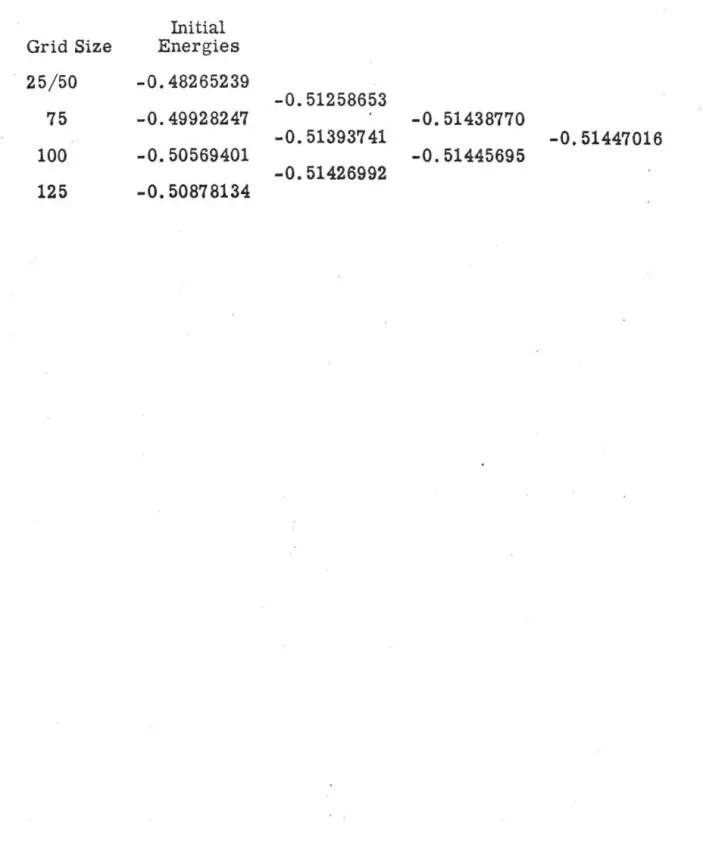
Grid

Size

9/20

.

25

30

35

40

45

50

55

60

TABLE

I.

The

S-limit

energy

of

the

helium

atom

ground

state.

Initial

Energies

-2.41777793

-2.78269471

-2.54914797

-2

.

86063837

-2.82599674

-2.87602834

-2.63374065

-2.87100304

-2.87862431

-2.8

4

80

4

064

-2.87797531

-2.87898631

-2.69059575

-2.87525177

-2.87891480

-2.87902636

-2.85994551

-2.87862484

-2.87901995

-2.87902778

-2.73028710

-2.87712569

-2.87899367

-2.87902759

-2.87903050

-2.8667327

4

-2.87886089

-2.87902601

-2.87903020

-2.75892384

-2.8780106

4

-2.87901638

-2.87902975

-2.87079279

-2.87895340

-2.87902882

-2.789238

40

-2.87845474

-2.87902

459

-2.8733

2566

-2.87899295

-2.79634490

-2.87869021

-2.87496

48

3

-2.80890225

23

TABLE II. The S-limit energy of the helium atom triplet

excited state.

Initial

Grid Size

Energies

20

/

50

-1.92155742

-2.14582478

75

-2.04615040

-2.17185406

-2.16534674

-2.17411134

100

-2.09829880

-2.17375017

-2 .17 425468

-2.17072494

- 2 . 1742 3 87 5

125

-2.12437221

-2.17411661

-2.17260920

24

TABLE

m.

The

S-limit energy of

the

hydride ion on the

linear grid.

Initial

Grid Size

Energies

.

25

/

50

-0.48265239

-0.51258653

75

-0. 49928247

-0.51438770

-0.

51393741

-0.51447016

100

-0.50569401

-0.51445695

-0.51426992

25

TABLE

IV.

S-limit energies for the helium atom and

the hydride ion on the square-root grid.

Grid Size

3/20

25

30

35

40

45

50

55

60

v'30/25

30

35

40

45

50

55

60

Helium

2nd Differences

-2.94612243

-2.923134

14

-2.910

42377

-2.

9026067 8

-2.89743538

-2.89382642

-2.89120257

-2.88923204

-2.88771261

Hydride

-0.

52387559

-0.52151323

-0.5

1996146

-0.51888329

-0.51810167

-0

.51751582

-0.51706469

4th Differences

-2.91652455

-2.90253697

-2.8951

4153

-2.89076150

-2.887954

43

-2.

8860477 8

-2.88

469360

-2.88369718

-2.88294265

-0.52

200314

-0.51960370

-0.5

1819644

-0.51730055

-0.51669

499

26

TABLE V. Polynomial fits for the helium atom S-limit.a

Second Differences

Grids Used in the

h2

h4 hs ...

h2 h3 h4 •..

h2 h4 h5 ...

Polynomial Fit

(20-25)

-2.88226607

-2.88226607

-2.88226607

(20-30)

-2.88095296

-2.88066116

-2.88095296

(20-35)

-2.88007081

-2. 87954872

-2.87997000

(20-40)

-2.87968114

-2.87930272

-2. 87955936

(20-45)

-2. 87946967

-2. 87918352

-2. 87935227

(20-50)

-2.87934222

-2,87912250

-2. 879237 38

(20-55)

-2.87926080

-2.87909307

-2. 87917124

(20-60)

-2.87920098

.

-2. 87903506

-2.87911356

Fourth Differences

(20-25)

-2.87767016

-2. 87767016

-2. 87767016

(20-30)

-2. 87886455

-2.87912997

-2.87886455

(20-35)

-2. 87898118

-2.87905020

-2. 87 899451

(20-40)

-2. 87901272

.

-2.87904011

-2. 87902257

(20-45)

-2.87902253

-2.87903181

-2.87902766

(20-50)

-2.87902500

-2.

87902523

-2.87902645

(20-55)

-2. 87902682

-2.87903194

-2. 87902896

(20-60)

-2. 87902886

-2.87903698

-2.87903236

27

TABLE VI.

Polynomial fits for the hydride ion S-limit. a

Second Differences

Grids Used

in

the

h h h ...

h

h

h

h

h

h~

...

Polynomial Fit

(30-35)

-0.51459713

-0.51459713

-0.51459713

(30-40)

-0.51479082

-0. 51474569

-0. 51479082

(30-45)

-0.51466352

-0.51457709

-0.51464655

(30-50)

-0.51460482

-0. 51453888

.

-0.51458322

(30-55)

-0. 51457261

-0.51452280

-0.51455157

(30-60)

-0.51454715

-0. 51448762

-0. 51452128

Fourth Differences

(25-30)

-0.51415043

-0.51415043

-0.51415043

(25-35)

-0.51445461

-0.51452703

-0.51445461

(25-40)

-0. 51447961

-0.51449563

-0.51448274

(25-45)

-0.51448779

-0.51449584

-0.51449060

(25-50)

-0.51448998

-0.51449172

-0.51449120

(25-55)

-0.51449188

-0.51449635

-0.51449370

(25-60)

-0.51449172

-0.51448720

-0.51449081

TABLE

Comparison

of

the

properties

predicted

by

the

S-limit

wavefunctions

to

the

radial

configuration

interaction

and

Hartree-Fock

results

for

He

and

H-.

Helium

(1s)

Hydride

Ion

Property

FD

RCf

HF

FD

RCf

RFC

E

-2.87903

-2.8790

0

-2.86168

-0.

51449

-0.51446

-0.4880

v

-5.

7581

-5.

7580

-5.7238

-1.

0290

-1.0289

V/E

2.0000

2.0000

2.0000

2.0001

2.0000

{l/r12>

0.

9867

0.9867

1.

0258

0.2983

(0.2973)

(1/r

1

+

l/r

3.3724

3.3724

3.

3748

.

1.

3273

-1.

3714

{

r1

+

r2

)

1.8690

1.

8688

1.8546

6.2079

6.207

5.0078

{

r

1

+

r

2

)

2.4221

2.4206

2.3696

34.

518

34.44

18.

821

aThe

basis

set

for

the

RC!

calculation

consisted

of

ls,

2s,

and

3s

Slater

orbitals

with

=

3.

7530

and

ls'

and

.

2s'

orbitals

with

=

1.

5427.

1\v.

A.

Goddard,

J.

Chem.

Phys.

48,

1008

(1968);

the

value

in

parenthesis

is

from

a

G

1

calculation.

cK.

E.

Baynard,

J.

Chem.

Phys.

48,

2121

(1968)

.

TABLE

VIIl.

Extrapolation

tables

for

the

angular

limits

of

the

helium

atom.

Grid

Size

9/20

25

30

35

40

45

50

9/20

25

30

35

40

45

50

P-Limit

-2.

44961031

-2.80393359

-2.5

7716669

-2.88179394

-2.84718934

-2.89746339

-2.65967361

-2.89234683

-2.90011414

-2.86930729

-2.89945145

-2.90047591

-2.71529071

-2

.

89667621

-2.90040445

-2.90051310

-2.88128120

-2.90011032

-2.90050715

-2

.75419473

-2.89858405

-2.90048148

-2.88811689

-2.90034786

-2

.78230185

-2.89948359

-2.89220890

-2.80318419

D-Limit

-2.45315095

-2.80642476

-2.5

8032952

-2.88406803

-2.84955991

-2.89970953

-2.66259436

-2.89460210

-2.90235548

-2.87162139

-2.90169399

-2.90271970

-2.71805051

-2.89892372

-2.90264776

-2.90275987

-2.88356616

-2.90235339

-2.90275344

-2.75684324

-2.90082909

-2

.

90272702

-2.89038608

-2.90259251

-2.78487075

-2.90172844

-2.894

4

6933

-2

.

80569448

Grid

Size

9/20

25

30

35

40

45

50

TABLE

VITI.

cont'd.

F-Limit

-2.45423836

-2.80714175

-2.58128358

-2.88465952

-2.85020718

-2.90026697

-2.66345468

-2.8S517066

-2.90290473

-2.87223011

-2.9022

4529

-l.90326875

-2.71884408

-2.89948176

"

-2.90319684

-2.90331188

-2.88415271

-2.90290315

-2.90330498

-2.75758829

-2.90138254

-2.90327795

-2.89095955

-2.90314302

-2.78557979

-2.90228038

-2.89503505

-2.80637629

G-Limit

9/20

-2.45471902

-2.80744677

25

-2.58170101

-2.88

489007

-2.85047082

-2.90047129

30

-2.66382512

-2.89538354

-2.90310098

-2.87246889

-2.90244355

-2.90346346

35

-2.71917959

-2.89968574

-2.90339186

-2.90350556

-2.88437626

-2.9030

9917

-2.9034988

2

40

-2.75789756

-2.90158

209

-2.90347208

-2.89117363

-2.90333783

45

-2.78586908

-2.90247752

-2.89524303

50

-2.80665013

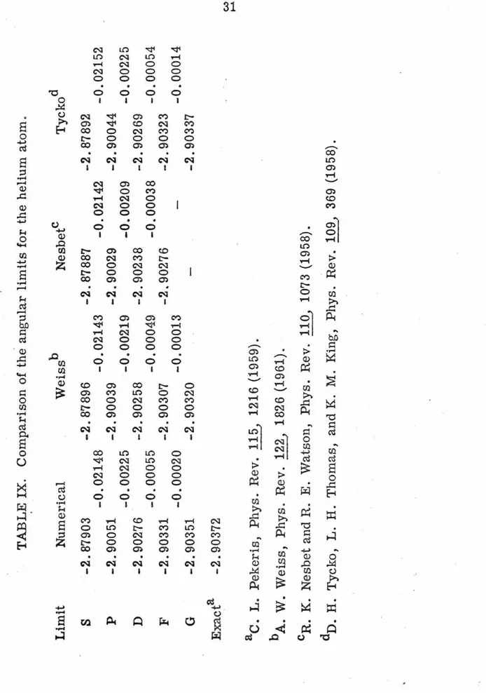
TABLE

IX

.

Comparison

of

the

angular

limits

for

the

helium

atom

.

Limit

Numerical

Weissb

Nesbetc

Tyckod

s

p

D

F

G

Exacta

-2.

87903

-0.02148

-2.90051

-0.00225

-2.90276

-0.00055

-2.90331

-0.00020

-2.90351

-2.90372

-2.87896

-0.02143

-2.90039

-0.00219

-2

.

90258

-0.00049

-2.90307

-0.00013

-2.90320

aC.

L.

Pekeris,

Phys.

Rev

.

115,

1216

(1959).

bA.

W.

Weiss,

Phys

.

Rev.

122,

1826

(1961).

-2.

87887

-0.

02142

-2.90029

-0.00209

-2.90238

-0.00038

-2.90276

cR.

K.

Nesbet

and

R.

E.

Watson,

Phys.

Rev.

110,

1073

(1958).

-2.

87892

-2.90044

-2.90269

-2.90323

-2.90337

d

.

D.

H.

Tycko,

L.

H.

Thom

as

,

and

K.

M.

King,

Phys.

Rev.

109,

369

(1958).

-0.02152

-0.00225

-0.00054

-0.00014

33

TABLE XI. Partial wave analysis of

the

energy for helium.

l

Tl

v

l

nuc

.

vi..

El..

0

2.877088

-6.732944

-5.768487

-2.891399

1

0.022998

-0.018653

-0.034538

-0.011490

2

0.002222

-0.000810

-0.002748

-0.000527

3

0.000542

-0.000110

-0.000615

-0.000073

4

0.000194

-0.000024

-0.000211

-0.000017

L;

2.903044

-6. 752541

-5.806599

-2.903506

34

TABLE

XII.

Partial wave

analysis of expectation

values for helium.

J..

(r1 + r2)

l

(r1 +r2>t

(l/r1

+

l/r

l.

~

(1 /r

i2>

l.t'

0

1.85014

2.37618

3.36647

0.96446

1

0.00837

0.01064

0.00933

0.01589

2

0.00039

0.00050

0.00041

0.00194

3

0.00006

0.00007

0.00006

0.00051

4

0.000013

0.000016

0.000012

0.00019

L;

1.

85897

2. 387

41

3.37627

0.94594

i

Exact a

1.85894

2.38697

3.37663

0.94582

35

Figure

1.

Contour and perspective plots of the S-limit for the

(ls

S and (ls2s)

3s

states of helium and the (ls

S state

of the hydride ion.

t£'..JUM r~ SfAIE S-Llt1l • Fl.tlCflON 1

• - TE S-L!HIT FLt.'CT!DN HELIUM fRIPLE1 ~TA

36

ll "UNCTION

HYOklO' /OH S-LIH .

Figure

1

t.=0.014

37

38

\

\

\

\

39

Figure 3

.

Contour plots of the functional coefficients for the helium

40

A=QQ64

=Q00044

Go

fijJJ&

5-f>R/H!Fl.. WAVE FOA Tt'E t'ELIUH ATOl1 _{P-PARTIRL WAVE FOR THE HELIUH ATOH}

0=000003

A=Q.000006

0-PRRTIRL WAVE FOR Tt'E HELIUH ATCJM F-PARTIRL WAVE FOR THE HEL!lhl ATOl1

G-PRRT I Fl.. WAVE FOR THE t£Lllhl ATCl'1

41

Figure 4. Perspective plots of the S- and P-wave functional coefficients

42

r

-

-

---

---

-

-i

L _

_

--

-

·

--

·

--

-

·

.

.

.

_

_

__

_

__

__

_

_

_

J

I

I

l_

S-PARTIAL ilRVE FCJR THE '1ELIUH ATOH

1'-f'fll\I lfll. i.ji1VE. ffJH IHF. llEl.!UH Hll'JH

43

A. INTRODUCT

I

ON

It

was previously shown that the functional coefficients of the

partial wave expansion for the first-order pair functions could be

obtained with the matrix finite difference (MFD) method.

1

Taking

the full electron interaction as the perturbation, the method has been

extended to the three pair equations that determine the first-order

wa vefunction for the lithium isoelectronic series. The pair functions

are independent of the nuclear charge and can be used to construct

the first-order wavefunctions for other atoms when the remaining

hydrogenic pair functions are determined.

2

The method is not

varia-tional and therefore can be applied without orthogonality constraints

to the excited pair functions that are not the lowest of their symmetry.

In

addition, the calculation of the total second- and third-order energy

involves none of the difficult integrals that occur for the complicated

variational functions containing interelectronic coordinates.

The first-order equation is reduced to its pair components in

the first section, using the theory developed by Sinanoglu

.

3

The pair

functions are then expanded in a partial wave series and the

coef-ficients are determined with the MFD method. The results found

using both the second difference and fourth difference approximations

are presented for the ground and excited states of the two-electron

atom. Finally, the total second- and third-order energies are

44

B. REDUCTION OF THE FIRST-ORDER E

With the entire electron interaction as the perturbation, the

dependence on the nuclear charge can be removed from the

perturba-.

tion equations. By scaling the radial distance to the nuclear charge

z

and measuring the energy in units of Z

the zero-order Hamiltonian

can be written,

l:

(-~v~

-

1/r.)

1 1

i

=

E

h.

1

(1)

i

and the perturbation becomes,

=

1/Z

2=

11r

lJ

..

(2)

In

these coordinates

the

expansion parameter is seen to be 1/Z and

accordingly the total energy and wavefunction can be expressed as

follows

,

E

=

(3)

·

where knowledge of

'11

is sufficient to determine

the

energy through

45

L

(4)

i

where

Q.

=-

~

'[

(-l)PP is the antisymmetrizer and

<Pi

are hydrogenic

.

p

spin-orbitals which satisfy hi

¢i

=

Eicpi.

For some states

'1:

will be

a

linear combination of determinants. The first-order equation is

L

(h. -

E.) '1'

=

(E

L

1/r

..

) '11

l

i

<j

(5)

with

Ei

=

<'lrol

I

1/r

..

'11

lJ

(6)

i <j

=

L

J

..

-

K ..

lJ lJ

i<j

and

46

1/r

..

)

'1>

lJ

=

C(,

L

<I>

lJ

.

.

(J .. -

lJ

--i_J

1/r

.

lJ

. }t(l - P

lJ

..

)¢.(i)¢.(j)

1

J

i

<j

(7)

where <I>ij is the orbital product without

¢i(i)

and

¢j(j).

The

permuta-tion

Pij

operates only on the particle labels. Equation

(7)

suggests

the

.

following form for

'11'

~l

=

a

L

<I>

..

t(

1 -

pi.)

w

.

. (

i'

j) •

lJ

J

lJ

(8)

i<j

Substituting into the first-order equation and making use of the orbital

equations, we obtain

<I> .

.

(h.

+

h. -

E.

-

E

.

)

t

(1 -

P

..

)

w

..

(ij)

=

lJ l

J

l

J

lJ

lJ

/J \ <I> ..

(J .. -

1/r

..

)t

(1 - P .. )

¢

-

(i)

<J>.(j)

(9)

vt

L

iJ

iJ

--i.J

iJ

iJ

i

J

A sufficient condition that

'11

satisfies (9) is

=

(1 O)

47

(<fl.

(1) ¢e(2)

I

J .. -

l/r

I

(1 - P

¢

.(1)

¢.

(2))

=

O (lla)

.

T

k

.

.

lJ

-lJ

l

J

·

where

</\_

(1) ¢

f.

(2) is any solution t

o

(h

+

h

J

(1)

¢

n

(2)

=

0 .

(llb)

For the ground state of the electron atom the following

three-pair equations must be solved,

(Jlsls - l/r

ls(l) ls(2)

(a[3 - [3

a

)

(12a)

(12b)

(J

1s2s - K1s 2s - l/r

(ls(1)2s(2) - ls(2)2s(1)

)

/

v'2

a

a

(J

1s 2s - l/r

(ls(l)

,8

~s(2)0!

-

ls(~)

/3

2s(l)

a

)

(12c)

Both (12a) and (12b) satisfy the exist

e

nce c

ond

ition

;

h

ow

ever, (12c) does

not, since the function (1 - P

ls(l)

a

2s(2)

,B

is a soluti

o

n

t

o (llb)

and (1s(1)a 2s(2)

,B

I

J

-48

metry states of the two-electron

atom,

(1 - P

ls(1){3 2s(2)a

=

i[

(ls(l)2s(2) - ls(2)2s(l))

(a{3

+

{3a)

-(ls(1)2s(2)

+

ls(2)2s(l)) (a{3

- {3a)J

(13)

(1 - P

F(l, 2){3a

=

T(l, 2)(a{3

+

{3a)/12

- S(1,.2)(l$ -

{3a)/12

'

an

equation for T(l, 2) is obtained which is identical to (12b) except

for the spin function, a.Tld the following equation is obtained for S(l, 2),

(ls(l) 2s(2)

+ 1s(2)

2s(l)

)/12

(a{3-

f3a)

(14)

The total first-order

function

can be

expressed in

terms of the

solutions to (12a), (12b),

and

(14) as follows,

'11

=

1/12

a(G(l, 2)

(a{3

- {3a)/12

2s(3)

a

+ [

T(l, 2)

(af3

+

{3a)/ 2

- S(l, 2)

(a{3 -

{3a)/

2) 1s(3)a

-

T(l,2)

aa

1s(3){3)

(15)

where

(11a)

is

satisfied

in

each

case.

The pair functions

G(l, 2),

T(l, 2),

and

S(l, 2)

are

identically

the first-order wavefunctions for

the (1sls)

S, (ls2s)

49

Because the pair functions G, T, and S are spherically

symmetric, the partial wave expansion for

each

is simply

(16)

By substituting this into the pair equation, multiplying both sides

by

Pe

(cos

8

and integrating over

the

angular variables, the

fol-lowing partial differential equation for u.Q(r

r

is obtained,

+

+

1)

/

2r~

+

+

1)

/

2r: -

Ei

=

(

E

(pair) 6

£

r f

r.Q )

1

R (r

r

(17)

where

E

=

5/8 for the (lsls) pair,

E

=

137/729 for the (ls2s)

8

pair, and

E

=

169

/

729 for the

(ls2s)

8 pair. The function R

~s

the

radial part of the zero-order function for each state

.

The boundary

conditions on u.Q(r

r

require

that

it

is finite for r

or r

=

0 and that

it

vanish for r

or r

=

oo.

The

set

of equations for the functional

co-efficients are not coupled and are solved

independently

for each

partial wave using the MFD method.

The details of the numerical analysis have already been

50

introduced which allow the diffuse excited states to be handled

efficiently. First, the radial cutoff (the point at which u

.Q

(r

r

is

required to vanish) for these states must be taken farther out than

.

for the (lsls) pair previously treated. Therefore, even with

ex-trapolation, a very large number of points are needed to achieve

comparable accuracy. To avoid this difficulty, the following

coor-dinate transformation was introduced into the pair equation,

(18)

The grid points in the transformed system are closely spaced near

the nucleus and farther apart in the tail regions, as viewed in the

untransformed system. This means that by using a large radial

cutoff and relatively few points, the regions important to the accurate

solution of (17) are not neglected.

The second modification in the MFD method was to improve

the difference approximation of the derivatives. Instead of truncating

the difference expansion at the second difference approximation, the

fourth difference is included giving the following improved

approxima-tion for the second derivative,

- lf •

u(Xo)

+

!

·

u(Xo - h) -

1

'J. •

u(Xo - 2h)

+

O(h

51

where his the grid size. The only difficult

y

occurs at the boundary

points, where (19) requires values of the function outside the defined

grid. This was resolved with the following approximations: at the

point x

=

xmax - h, where xmax is the radial cutoff, u(x

+

2h) was

set to zero, and at x

=

h the value u(x - 2h) was set equal to u

(

x).

The latter assumption was arrived at by investigating the power

series form of u(x) for small x and can be shown to introduce an

error of the order of the difference truncation error, if the

coordi-nate transformation (18) is used.

An

alternative would be to use

the usual second difference approximation at the boundaries and the

fourth difference approximation elsewhere. Actually both approaches

were used, depending on which method was used to solve the difference

equations.

When substituted into (17), both the second difference and

the fourth difference approximations lead to a set of simultaneous

equations of the form

D

·u

=

b

(20)

where D is a banded matrix. The second difference approximation

produces a symmetric matrix, as does the fourth difference

approxi-mation with the modified boundary conditions. However, the mixed

difference method leads to an unsymmetric matrix. The difference

equations were solved with Gaussian elimination for the

=

0 partial

52

for the higher partial wave equations

the

Gauss-Seidel

method

con-verged extremely fast, while

for

the S-wave the

method

diverged.

Because the Gaussian elimination

method

is more

efficient

for

sym-metric matrices, the mixed difference approximation was not used

for

the S-wave, but was used for each of the higher waves.

D.

CALCULATION OF THE SECOND-

AND

THIRD-ORDER

ENERGIES FOR THE TWO-ELECTRON STATES

The partial-wave equations

for

each

pair

function

were

solved

using both the usual second difference approximation and

the improved

difference formula given by (19). The second-order energy for each

pair was found from

(21)

The radial integral

was

calculated by

the trapezoidal rule.

The

calculations

were carried

out

at several grid

sizes

and the results

extrapolated

with

Richardson

rs 8

method. Therefore,

the

dHference

and quadrature errors

were eliminated

in one step.

The extrapolation

tables for the

partial

wave

contributions

to E

for the

(lsls) pair are

given in

Table

I.

The results

were

untrans-53

formed (linear) grid with a 12 a. u. cutoff. The first column of each

table lists the number of strips used in each direction. The second

column gives the initial results and the remaining columns contain

the extrapolants. The latter were obtained using different sets of

results from the first column. By displaying the results in this

manner,

it

is possible

fo

determine

if

the extrapolants are converging

from above or below the true value. The partial wave contributions

from all but the S-wave are converging from below and have

to at least six decimal places. The results for the S-wave appear to

oscillate

,

but the sub-table produced by the 45, 60, and 75 strip

cal-culations is converging smoothly from below. The extrapolation

tables for the

S and

S excited states are given in Tables II and III.

These results illustrate the need for the modifications that were

dis-cussed in section C. The 120 strip S-wave calculation required the

solution of nearly 14, 000 linear equations which took about one hour

on

·

the IBM 360-75. The S-wave cutoff was taken at 24 a. u., which

was still not far enough from the nucleus. Clearly it was not practical

to re-solve the equations wit