COMPARISON OF CORONAL EXTRAPOLATION METHODS FOR CYCLE 24 USING HMI DATA
William M. Arden1, Aimee A. Norton2, Xudong Sun2, and Xuepu Zhao2
1
University of Southern Queensland, Toowoomba, Queensland, Australia
2
Hansen Experimental Physics Laboratory, Stanford University, Stanford, CA 94305, USA Received 2016 January 13; accepted 2016 March 10; published 2016 May 17
ABSTRACT
Two extrapolation models of the solar coronal magneticfield are compared using magnetogram data from theSolar Dynamics Observatory/Helioseismic and Magnetic Imager instrument. The two models, a horizontal current– current sheet–source surface(HCCSSS)model and a potentialfield–source surface(PFSS)model, differ in their treatment of coronal currents. Each model has its own critical variable, respectively, the radius of a cusp surface and a source surface, and it is found that adjusting these heights over the period studied allows for a better fit between the models and the solar openflux at 1 au as calculated from the Interplanetary Magnetic Field(IMF). The HCCSSS model provides the betterfit for the overall period from 2010 November to 2015 May as well as for two subsets of the period: the minimum/rising part of the solar cycle and the recently identified peak in the IMF from mid-2014 to mid-2015 just after solar maximum. It is found that an HCCSSS cusp surface height of 1.7Re
provides the bestfit to the IMF for the overall period, while 1.7 and 1.9Regive the bestfits for the two subsets. The corresponding values for the PFSS source surface height are 2.1, 2.2, and 2.0Rerespectively. This means that the HCCSSS cusp surface rises as the solar cycle progresses while the PFSS source surface falls.
Key words:solar wind–Sun: activity–Sun: corona–Sun: heliosphere–Sun: magneticfields–Sun: photosphere
1. INTRODUCTION
Modeling solar coronal openflux is one of the tools available to solar physics in the search for understanding the behavior of the corona. This is important, in turn, because of the corona’s influence on space weather and Earth’s magnetosphere.
One class of these models involves the extrapolation of the coronal magnetic field and the interplanetary magnetic field (IMF) from the photospheric magnetogram. Early models achieved good results with simple, current-free models (Schatten et al. 1969); later versions include the effects of coronal currents (Hoeksema et al. 1983). Today, the Helio-seismic and Magnetic Imager (HMI) on board the Solar Dynamics Observatory (SDO) provides magnetograms at a high cadence, but photospheric magnetic data has been available for many years, beginning with the work of Hale (1908)and continuing through the full-disk magnetograms of Babcock(1963)in the 1950s and 1960s to current instrumenta-tion such as HMI. Coronal models made use of this data as early as the 1960s(Schatten et al.1969), and an improved form of these models (the Wang-Sheeley-Arge, or WSA model; Arge & Pizzo 2000) is currently used by the NOAA Space Weather Prediction Center(SWPC)in forecasting the magneto-spheric effects of solar activity.
Since these early developments, increases in computing power have enabled more sophisticated modeling of the corona through magnetohydrodynamic approaches. Extrapolation models provide comparable results (Riley et al. 2006) and can be quickly and easily implemented with small-scale computing resources. Extrapolation models lend themselves to computing the long-term, relatively smooth quasi-static magnetic field at the corona.
This paper compares two such extrapolation models: a potential field–source surface(PFSS) model developed at the Lockheed Martin Solar and Astrophysics Laboratory(LMSAL; Schrijver & DeRosa 2003) and a horizontal current–current sheet–source surface(HCCSSS)model developed at Stanford University (Zhao & Hoeksema 1994, 1995). The solar open
magneticflux calculated by the models is compared to the open flux derived from the IMF using a technique proposed by Lockwood(2002). The analysis in this paper builds on earlier work by the authors(Arden et al.2013; Arden & Norton2015). In this paper, we examine HMI data for the period from 2010 November 26 to 2015 May 21, which encompasses the rising phase of solar cycle 24 and the dramatic increase in the solar meanfield and openflux observed by Sheeley & Wang(2015)
which began in mid-2014. As those authors point out, this type of rise has characterized the declining phase of at least the last three solar cycles. This is particularly interesting since it has been shown that open flux during the declining phase is a reliable precursor of the activity in the next solar cycle (Feynman1982).
This paper begins with an outline of the data and analytical methods used. It continues with descriptions of the two models and the method of calculating the open flux at 1 au. The performance of the two models is compared and the results are discussed in thefinal sections of the paper.
2. DATA AND METHODOLOGY
Coronal extrapolation models such as these begin with measured magneticfield data from photospheric observations. Field lines originating at the photosphere are mathematically extrapolated upward to the corona and beyond to an imaginary source surface outside of which all of thefield lines are forced to be open and radial. Both models used in this paper follow this general approach, with the differences described in detail in Sections 2.2 and 2.4. Table 1 presents an abbreviated comparison of the two models.
A test of the accuracy of these models is a comparison to the openflux at Earth, i.e., 1 au from the Sun. The IMF at Earth provides an in situ measurement of open flux; the IMF is measured by spacecraft such as ACE and made publicly available in NASA’s OMNI 2 database.
2.1. Magnetograms—the Photospheric Field
The SDO/HMI instrument produces full-disk, line-of-sight magnetic images with a cadence of 45 s from the front camera and 12 minutes from the side camera. The 12 minute images are used in this study (HMI.M-720 s data series,http://jsoc. stanford.edu/jsocwiki/hmi.M-720s-info). Even a full-disk image, however, only covers the Earth-facing half of the photosphere; accurate calculation of the total openflux requires information about the entire photosphere. Therefore, a set of sequential images over a solar revolution is typically combined to form a synoptic map of the entire Sun. While these images do not represent the Sun at any one time (the earliest data incorporated into the synoptic map is approximately 27 days older than the latest data), they are sufficient as input for the quasi-static models discussed here.
In addition to the time-dependence of the measurements, the difficulty of measuring the magneticfield at large line-of-sight projection angles is well known (Petrie 2012). These large angles occur at high solar latitudes, which makes them critical for accurate modeling; the unipolar magnetic regions at high latitudes comprise the polar caps where much of the high-speed solar wind originates. Sun et al. (2011)discuss the difficulties involved with this problem, and some possible solutions.
Both of the models tested here are fundamentally based on spherical harmonic integration, and thus require some estimate of the surface magnetic field over the entire photosphere. The two models use different methods to arrive at the magnetic fields at high latitudes (which are difficult to measure accurately). The LMSAL/SSW PFSS model uses a fl ux-dispersal model to estimate the polar magneticfield(Schrijver & DeRosa2003). The HCCSSS model incorporates polarfield observation in the fall and spring (when the solar tilt angle is favorable) and estimates the values at other times through spatial-temporal interpolation (Sun et al.2011).
This work uses synoptic maps from LMSAL as input to the PFSS model. These are publicly available athttp://www. lmsal.com/solarsoft/archive/ssw/pfss_links_v2/. Synoptic maps used as input for the HCCSSS model were obtained from Stanford University(Sun et al.2011).
2.2. Potential Field Source Surface(PFSS)Model
The use of the solar magnetic field measured at the photosphere as the lower boundary condition for a coronal model is well established. Beginning with early work by Altschuler & Newkirk(1969) and Schatten et al.(1969), and continuing through work by Schrijver & DeRosa(2003) and many others, these models have reached a level of sophistica-tion that enables them to be used for near-real-time space weather prediction by the NOAA SWPC (Arge & Pizzo
2000; see, for example,http://www.swpc.noaa.gov/products/ wsa-enlil-solar-wind-prediction). Mackay & Yeates (2012)
provide an overview of many of these models.
The corona is known to carry electric currents, but these currents are generally not significant on global scales, except near the heliospheric current sheet. The lower boundary condition for the model is the photosphericfield derived from magnetograms(with radius equal to that of the Sun,Re). This field depends on radial distance as well as solar latitude and longitude (R=B r, ,( q f)). An imaginary sphere called the source surface, at radius Rss where the magnetic field is
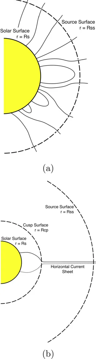
assumed to be purely radial(Rss=B r( )), provides the upper boundary condition. As its name implies, the PFSS technique does not consider coronal currents below the source surface. Figure1(a)shows a schematic of the PFSS model.
Under these constraints, ´B=0andB= -Y, where
Ψis a scalar potential(see Mackay & Yeates2012).Ψsatisfies Laplace’s equation:
( )
Y =2 0 1
with boundary conditions
( q f) ( )
¶Y
¶r = =
-B R, , 2
r R
r s
s
and
( )
q f
¶Y
¶ =
¶Y
¶ =
= =
0. 3
[image:2.612.42.568.75.287.2]r Rss r Rss
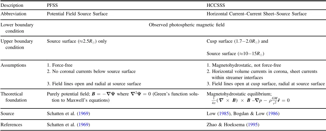
Table 1
Comparison of Extrapolation-based Coronal Magnetic Field Models
Description PFSS HCCSSS
Abbreviation Potential Field Source Surface Horizontal Current–Current Sheet–Source Surface
Lower boundary condition
Observed photospheric magneticfield
Upper boundary condition
Source surface(»2.5R)only Cusp surface(1.7−2.0R)and Source surface(≈10−15R)
Assumptions 1. Force-free 1. Magnetohydrostatic, not force-free
2. No coronal currents below source surface 2. Horizontal volume currents in corona, sheet currents within streamer interfaces
3. Field lines open and radial at source surface 3. Field lines open at cusp surface, radial at source surface
Theoretical foundation
Purely potentialfield;B= -Ywhere Y2 =0(Green’s function solu-tion to Maxwell’s equations)
Magnetohydrostatic equilibrium;
( ´ ) ´
p B B
1
4 –p-r ˆr=0
GM r2
Source Schatten et al.(1969) Low(1985), Bogdan & Low(1986)
This equation is solved using spherical harmonic methods to provide the components of B r, ,( q f) at any point over the rangeRs r Rss.
The PFSS model used in the present study was developed at LMSAL. It uses the SolarSoft (IDL) software package and assimilates surface-flux estimates along with MDI and HMI magnetogram data. This model is currently in its second revision(http://www.lmsal.com/forecast/).
The output of a PFSS model includes values of the radialB
field(Br, in nT)over a grid at the source surface. The total open
flux is obtained by integrating the absolute values of the radial field over the sphere and then dividing by two (simply integrating theBfield would result in zero netflux). In actual computations, this integration is half the sum of the absolute values weighted by the area of the respective grid elements.
Synoptic magnetograms of the photosphere at a cadence of one per day are used as input to the PFSS model. The output is a dailyfile of theBfield as described above.
2.3. Varying the PFSS Source Surface for Better Fit
The source surface height Rss is commonly taken to be
2.5Re(Hoeksema et al.1983). However, in fact, this is a free parameter in the PFSS model. Varying the height of the source surface over the course of the solar cycle has been explored by Lee et al.(2011)and Arden et al.(2013). AdjustingRssis one way to better match the open flux measured at 1 au. After examination of source surface heights ranging in value from 1.5 to 2.5Re, the values chosen for this study are 2.0 and 2.25Refor different phases of the solar cycle.
The connection between the source surface height and open flux is as follows. Smaller spatial-scale magnetic loops that close lower in the atmosphere are represented by the higher spherical harmonic orders. Loops that close beneath the source surface(and therefore do not penetrate it)do not contribute to the openflux above the source surface. As the source surface height is raised, therefore, fewer of the higher-order loops penetrate the source surface and the openflux decreases. As the source surface height is lowered, more of these higher spatial-order loops cross the source surface and the open flux increases.
In Arden et al.(2013), it was shown that moving the source surface to higher values in the PFSS model gives a betterfit as the solar cycle passed from maximum to minimum. The results of the current study support that conclusion(see Section4).
2.4. Horizontal Current–Current Sheet–Source Surface
(HCCSSS)Model
[image:3.612.88.248.59.653.2]The HCCSSS model takes a different approach to modeling the corona. This model begins with the assumption of a corona in magnetohydrostatic equilibrium with horizontal electric currents instead of a potential field, and adds a cusp surface to model the effect of streamer current sheets (Zhao & Hoeksema1994,1995). This model, unlike PFSS, is not force-free due to the inclusion of pressure and gravity. Finally, the HCCSSS model adds a source surface to include volume currents beyond the cusp surface. The resulting model derives its name from the inclusion of horizontal currents, a current sheet, and a source surface. Note that in Zhao & Hoeksema (1995), this model is called CSSS; the name HCCSSS is more descriptive and will be used here.
As described by Zhao & Hoeksema, helmet-streamer structures such as those observed in solar eclipses indicate that coronal currents alter the magnetic topology. A streamer interface starts near the cusp-shaped neutral point over a closed region. Coronal currents are assumed to have two components: horizontal volume currents in the corona and sheet currents flowing within streamer interfaces. All of the helmet-streamer components are assumed to have identical heights(r=Rcp, the
“cusp height”). The corona is then divided into two regions separated by a spherical surface located atRcp, called the“cusp
surface.”Magneticfield lines are assumed to be closed below the cusp surface and open(but not necessarily radial)above it. The outer region is bounded by a“source surface” correspond-ing to the similarly named surface of the PFSS model, at which the magnetic field lines are both open and radial. Figure1(b) depicts the HCCSSS model. See Table1 for a comparison of the PFSS and HCCSSS models.
The HCCSSS model(Zhao & Hoeksema1994)begins with the equation for magnetohydrostatic force balance in 1 r2
gravity(Bogdan & Low1986):
( ) ˆ ( )
p ´B ´B-p -r r=
GM r 1
4 2 0, 4
whereBis the magneticfield,pis the plasma pressure, andρis the plasma density. Bogdan & Low (1986) found that this equation has a set of solutions that depend on the function
( q f)
F r, , :
( ) ˆ ˆ ˆ ( )
h
qq q ff
= - ¶F
¶ -¶F ¶ -¶F ¶ B r
rr r r
1 1
sin 5
( ) ( )[ ( )] ( )
ph h
= + - ¶F
¶ ⎜ ⎟ ⎛ ⎝ ⎞ ⎠
p p r r r
r 1
8 1 6
0
2
( ) ( ) ( )
( )[ ( ) ]
( )
r r h
p q p
h q
f p h h
= + - ¶ ¶ ¶F ¶ + - ¶ ¶ ´ ¶F ¶ + ¶ ¶ -¶F ¶ ⎜ ⎟ ⎜ ⎟ ⎪ ⎪ ⎧ ⎨ ⎩ ⎛ ⎝ ⎞ ⎠ ⎛ ⎝ ⎜ ⎞ ⎠ ⎟ ⎡ ⎣ ⎢ ⎛⎝ ⎞⎠⎤ ⎦ ⎥⎫⎬ ⎭ r GM r r r r r
r r r r
1 1 8 1 8 1 sin
8 1 ,
7 0
2
2
2 2 2
where
( ) ( )
h =⎜⎛ + ⎟ ⎝ ⎞⎠
r a
r
1 . 8
2
Solutions for each of the two regions are formulated with the constraint that all three components of the magnetic field be continuous across the cusp surface. Further details can be found in Zhao & Hoeksema (1994). In actual computations, only a
and Rcp, along with the observed photospheric magnetic field,
are required to calculate the magnetic field above the photo-sphere. In this paper, the value of a is chosen to be 0.2, as described in Zhao & Hoeksema(1995). It is below this height that the horizontal currents primarily flow. The model is relatively insensitive to the choice of Rss, the source surface
height (which corresponds to the base of the heliosphere); values of 10–15 were tested in this research with little difference in the final results for the open flux. In agreement with Zhao & Hoeksema(2010), a value of 15Rewas chosen. Cusp surface heights of 1.5, 1.7, 2.0, and 2.2Rewere explored. In its present form, the HCCSSS model takes as input synoptic maps of the photosphere at a cadence of one
Carrington Rotation (CR). The output is thus an average of openflux over that CR.
In a technique similar to that employed in the PFSS model, the openflux calculated by the HCCSSS model can be adjusted by moving the cusp surface higher(which decreases openflux) or lower(which increases openflux).
2.5. Open Flux at 1 au—IMF at Earth
Thanks to the work of Lockwood(2013)and others, there is a direct way to arrive at an estimate of the open magneticflux at 1 au. This method is based on values of Br, which are
available from the OMNI 2 database (http://omniweb.gsfc. nasa.gov/ow.html). This database was created in 2003 and contains in situ solar wind magneticfield and plasma data from a number of near-Earth spacecraft at a one-hour cadence. It includes IMF data from 1963 November through the present; all three components of thefield(Bx,Byand Bz)are given, in
units of nT. We take Bx, the magneticfield component along the Sun–Earth line, to be equal to the radialfield, and use data from 2010 November through 2015 May. Daily averages, which are also found in the OMNI 2 database, are used in our calculations and then averaged by CR to correspond to the output of the HCCSSS model.
The radial component of the heliospheric magneticfield has been shown to be independent of heliospheric latitude; this was deduced from measurements by theUlysses spacecraft(Smith & Balogh1995; Smith2008,2011). Based on this assumption, the total unsignedflux passing through a sphere with a radius of 1 au(R1)can be given simply by
∣ ∣ ( )
p
=
F 4 R B1 r 2, 9
2
as shown by Lockwood(2002). Note that the factor of two is required for the following reason. If the total openflux over a sphere at 1 au is calculated from the IMF measured at Earth, then all of theflux over the whole sphere will be presumed to be of that sign. Taking the absolute value of Br removes the
sign of the polarity, but effectively makes all of the flux positive. The net open flux must be zero, and so division by two is required since both the positive and negativeflux would otherwise be counted as positive—resulting in a value that is twice the actual one. In the paper, we chose to call this flux “unsigned”since it represents theflux of both polarities.
2.6. Comparing IMF to Modeled Open Flux
We compare the calculated IMF at 1 au with the results of the PFSS and HCCSSS models over the time period from 2010 November 26 through 2015 May 21, which corresponds to CR 2104–2163. As described earlier, the HCCSSS model is currently based on synoptic maps of one CR. The PFSS and IMF data are therefore binned by CR by averaging daily values over corresponding periods. Goodness of fit is determined by calculating the rms value of the difference between the open flux derived from the IMF and each model over all of the CRs in the period.
increase in the Sun’s dipole moment(Sheeley & Wang2015). While Sheeley & Wang point out that this pattern has occured after solar maximum in each of the three previous solar cycles, it is not as widely known as other aspects of the solar cycle; it does not appear in common measures of solar activity such as sunspot count, for example. During this period, the strength of the IMF radial component doubled; this increase is readily apparent in our data, and it seemed appropriate to break our tests of the models into two parts—one for the relatively calm period from late 2010 through mid-2014, and one for the rise (and subsequent fall) of the IMF from mid-2014 to mid-2015.
3. RESULTS
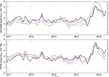
Figure2 shows the unsigned open flux computed from the IMF compared to the outputs of the HCCSSS and PFSS models, each at two different cusp surface or source surface heights. In these plots, the average value of the IMF-based or modeled openflux is plotted using one point per CR for visual comparison. With a cursory glance, both models track at least the gross features of the IMF when averaged at one CR, including the 2014–2015 peak in the IMF. The HCCSSS model with a cusp surface height of1.7Rappears to follow the IMF
better from the beginning of the period up to the middle of 2014(when the IMF rose dramatically), but then overestimates the open flux during the IMF peak. The PFSS model gives varying results; a source surface height of 2.2Regives a closer visualfit over the earlier part of the period, but 2.0Reappears closer in the later part(the peak of cycle 24).
For a more quantitative measure, we calculate the difference between the modeled openflux and the IMF openflux, one CR at a time, and then compute the rms value of the collective differences. These values are shown in Table 2 for three different subsets of data—the entire period from 2010
November 26 to 2015 May 21 (CR 2104–2163), the quasi-steady state period from 2010 November 26 to 2014 July 24 (CR 2104–2152), and the period of the IMF surge from 2014 July 25 to 2015 May 21(CR 2153–2163).
The results in Table2 can be summarized as follows.
1. Overall, a cusp surface height of1.7Rin the HCCSSS
model gives the bestfit from either model for the entire period under study. Setting the source surface height to
R
2.1 in the PFSS model gives the bestfit for that model, but the fit is not as good as that achieved with the HCCSSS model.
2. For the relatively uneventfulfirst epoch, CR 2104–2152, the HCCSSS model with a cusp surface height of1.7R,
again gives a betterfit than any of the three PFSS source surface heights. The best PFSS source surface height is2.2R.
3. During the peak in the IMF, CR 2153–2163, the HCCSSS model with a 1.7R cusp surface height
overestimates the IMF openflux; raising the cusp surface height to 1.9R lowers the model’s open flux and
provides a betterfit. On the other hand, the PFSS model underestimates the IMF open flux; lowering the source surface height from 2.2R to 2.0R raises the model’s
openflux to match more closely the IMF openflux.
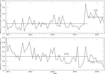
[image:5.612.128.488.52.305.2]Figure3 illustrates the variation in the optimal cusp surface and source surface heights. Here, interpolated values of the cusp surface and source surface heights that give the bestfit to the IMF openflux are shown for each CR. Reference values of 1.7Reand 1.9Reare shown for the HCCSSS model as well as values of 2.0Re and 2.2Re for the PFSS model, in their corresponding epochs. OMNI data from 2014 July shows a drop in IMF openflux just before the striking increase which resulted in the to-date solar cycle 24 maximum IMF value of
Figure 2.IMF, HCCSSS, and PFSS unsigned openflux. In both plots, the heliospheric openflux calculated from the IMF OMNI 2 database is plotted by the black line. Top: HCCSSS openflux is plotted against IMF openflux for HCCSSS cusp surface heights of1.7R(upper line, blue)and1.9R(lower line, red). Bottom: PFSS
5.2×10²²Mx in 2014 November. Thefirst and second epochs are divided so that 2014 July is included in thefirst epoch(CR 2104–2152)because the IMF did not reach values higher than average until 2014 August. For the HCCSSS model (upper plot, Figure 3), the overall mean cusp surface height of the interpolated values is 1.7Re. For the first epoch, the mean height is also 1.7Re while for the second epoch it is 1.9Re. The corresponding mean source surface heights for the PFSS model(lower plot, Figure3)are 2.1, 2.2, and 2.0, respectively. All of these values are represented in Table 2.
4. DISCUSSION AND CONCLUSIONS
The ideal coronal extrapolation model would allow for the initial specification of parameters such as source surface height or cusp surface height, and would then reproduce coronal behavior precisely as the photospheric inputs change. Attempts to develop such a model lead to open questions as well as open flux. What are the optimum heights of the cusp surface and source surface, and when should they be changed? Why does a model work well under some circumstances but need
modification in others? The recent work of Sheeley & Wang (2015)describing an unexpected rise in the IMF in late 2014 provides us with the opportunity to study these models in both quasi-steady state and widely varying situations. Wefind that both of the models require modification of a primary variable in order to track the IMF accurately in both the rising phase (2010–2014) and the post-maximum IMF peak: cusp surface height in the case of the HCCSSS model, and source surface height for the PFSS model.
Over the course of the period studied, the mean value of the CR-averaged IMF was 2.9´1022 Mx. Table 2 includes the
[image:6.612.42.567.76.183.2]percent error (100% × rms difference/mean IMF) for the values of the cusp surface and source surface. It is clear that the HCCSSS model gives at least a slightly better, and in some cases significantly better,fit than the PFSS model in all cases; the smallest errors for the entire period, the rising phase of cycle 24, and the IMF peak in the declining phase all result from the use of the HCCSSS model. Both models, however, are capable of errors of 20% or less with appropriate tuning of the source surface/cusp surface heights.
Table 2
Rms Value of(IMF−Coronal Model)Difference and(Percent Difference)Between Mean IMF and Model, Over CR 2104–2163
Period(CR) Dates IMF–HCCSSS IMF–PFSS
(rms×1021Mx) (rms×1021Mx)
Cusp Surface Height Source Surface Height
1.7Re 1.9Re 2.0Re 2.1Re 2.2Re
2104–2163 2010 Nov 26–2015 May 21 5.31(18%) 7.00(24%) 5.77(20%) 5.4(19%) 5.76(20%) 2104–2152 2010 Nov 26–2014 Jul 24 4.39(15%) 7.52(26%) 5.79(20%) 5.07(18%) 4.97(17%) 2153–2163 2014 Jul 25–2015 May 21 8.28(29%) 4.08(14%) 5.90(20%) 6.88(24%) 8.57(30%) Note.Values in bold are the minimum difference in RMS(and percent), i.e., the bestfit between the model and the observed IMF.
[image:6.612.128.487.218.469.2]The results of this study can be compared to the conclusions of an earlier article by the authors(Arden et al.2013). In that work, it was found that a higher PFSS source surface during solar minimum resulted in a betterfit to the openflux at 1 au as calculated from the IMF. The source surface was lowered as maximum approached, which improved the fit. The NOAA SWPC estimates that the current solar cycle began in early 2009 and reached its peak in the first half of 2014 (http:// www.swpc.noaa.gov/products/solar-cycle-progression). The current study begins in 2010, soon after minimum, and we find that a higher source surface value does, indeed, give a better fit for thefirst part of the study(2010 November–2014 July)—the minimum and rising phases of cycle 24. Lowering the source surface improves thefit during the period from 2014 July to 2015 May—the period of solar maximum and the peak in the IMF, and the end of this study.
We find that the opposite is true for the HCCSSS model, whose critical parameter is the height of the cusp surface and which introduces a more sophisticated treatment of coronal currents. It is similar to the PFSS model in the respect that raising the cusp surface lowers the calculated openflux. Since the model overestimates the open flux during the IMF peak, raising the cusp surface as maximum approached yields a better fit to the IMF openflux.
The choice of epochs notwithstanding, examination of Figure 2 reveals that the starting HCCSSS cusp surface of
R
1.7 provides a betterfit for a longer time(2010 to mid-2014) than the starting PFSS source surface height of2.25R, which
begins to deviate significantly from the IMF openflux in mid-2013—as maximum approaches. In other words, the time at which the source surface needs to be lowered (mid-2013) is distinctly different from the time that the cusp surface needs to be raised (mid-2014).
This paper examines the effect of changing the HCCSSS cusp surface and PFSS source surface heights. With regard to the HCCSSS model, in particular, it is expected that all three free parameters of the model (the variable a, cusp surface height, and source surface height)probably vary over the solar cycle, and this variation could significantly affect the calculated results. It is appropriate to continue this study to find the optimum values of all three parameters. Also, while there is no physical surface against which the PFSS source surface height can be tested, validation of the average HCCSSS cusp surface height reported here by comparison to the cusp height of streamers as observed in coronagraph data could be a profitable avenue for future exploration.
We have focused here on the behavior of two models and demonstrated that critical parameters in each model must be adjusted to fit the IMF at Earth. We have not addressed the reasons why these adjustments are necessary. We believe that the answer lies largely in the phenomena which affect the solar magnetic field on its way from the Sun to 1 au, including
coronal mass ejections(Owens & Crooker2006; Owens et al.
2011; Schwadron et al. 2010). These phenomena are not modeled by either technique—or, for that matter, by any method based on the extrapolation of the photospheric magnetic field. While the authors believe that most of these transient effects are averaged out over time periods on the order of one CR, this remains very much an area for further research and discussion.
Allowing the parameters of a model to change over the course of the solar cycle enables us to more closely model the IMF openflux in retrospect, but at the cost offinding a single value that could be used predictively in fields such as space weather forecasting. The search continues for a model which captures the most significant aspects of the corona’s complex and dynamic behavior without needing to adjust surface heights or other variables.
The authors wish to acknowledge J. Todd Hoeksema of Stanford University and Marc DeRosa of LMSAL for their assistance in the research that led to this paper. The OMNI data were obtained from the GSFC/SPDF OMNIWeb interface athttp://omniweb.gsfc.nasa.gov.
REFERENCES
Altschuler, M. D., & Newkirk, G., Jr. 1969,SoPh,9, 131
Arden, W. M., & Norton, A. A. 2015, in Triennial Earth–Sun Summit(poster presentation)
Arden, W. M., Norton, A. A., & Sun, X. 2013,JGRA,119, 1476
Arge, C. N., & Pizzo, V. J. 2000,JGR,105, 10465
Babcock, H. W. 1963,ARA&A,1, 41
Bogdan, T. J., & Low, B. C. 1986,ApJ,306, 271
Feynman, J. 1982,JGR,87, 6153
Hale, G. E. 1908,ApJ,28, 315
Hoeksema, J. T., Wilcox, J. M., & Scherrer, P. H. 1983,JGR,88, 9910
Lee, C. O., Luhmann, J. G., Hoeksema, J. T., et al. 2011,SoPh,269, 367
Lockwood, M. 2002, in ESA SP-508, SOHO 11 Symp., From Solar Min to Max: Half a Solar Cycle with SOHO, ed. A. Wilson (Noordwijk, Netherlands: ESA Publications),507
Lockwood, M. 2013,LRSP,10, 4
Low, B. C. 1985,ApJ,293, 31
Mackay, D. H., & Yeates, A. R. 2012,LRSP,9, 6
Owens, M. J., & Crooker, N. U. 2006,JGR,111, A10104
Owens, M. J., Crooker, N. U., & Lockwood, M. 2011,JGR,116, A04111
Petrie, G. J. D. 2012,SoPh,281, 577
Riley, P., Linker, J. A., Mikic, Z., & Lionello, R. 2006,ApJ,653, 1510
Schatten, K. H., Wilcox, J. M., & Ness, N. F. 1969,SoPh,9, 442
Schrijver, C. J., & DeRosa, M. L. 2003,SoPh,212, 165
Schwadron, N. A., Connick, D. E., & Smith, C. 2010,ApJL,722, L132
Sheeley, N. R., Jr., & Wang, Y.-M. 2015,ApJ,809, 113
Smith, E. J. 2008, in The Heliosphere Through the Solar Activity Cycle, ed. A. Balogh, L. J. Lanzerotti, & S. T. Seuss(Chichester, UK: Praxis),79
Smith, E. J. 2011,JASTP,73, 277
Smith, E. J., & Balogh, A. 1995,GeoRL,22, 3317
Sun, X., Liu, Y., Hoeksema, J. T., Hayashi, K., & Zhao, X. 2011,SoPh,270, 9
Zhao, X. P., & Hoeksema, J. T. 1994,SoPh,151, 91
Zhao, X. P., & Hoeksema, J. T. 1995,JGR,100, 19