Truly eccentric - II. When can two circular planets mimic a single eccentric orbit?

Advance Access publication 2019 January 23

Truly eccentric – II. When can two circular planets mimic a single

eccentric orbit?

Robert A. Wittenmyer ,

Christoph Bergmann ,

Jonathan Horner,

Jake Clark

and

Stephen R. Kane

1_{Centre for Astrophysics, University of Southern Queensland, Toowoomba, QLD 4350, Australia} 2_{Exoplanetary Science at UNSW, School of Physics, UNSW Sydney, NSW 2052, Australia}

3_{Department of Earth Sciences, University of California Riverside, 900 University Avenue, Riverside, CA 92521, USA}

Accepted 2019 January 17. Received 2019 January 16; in original form 2018 November 9

A B S T R A C T

When, in the course of searching for exoplanets, sparse sampling and noisy data make it necessary to disentangle possible solutions to the observations, one must consider the possibility that what appears to be a single eccentric Keplerian signal may in reality be attributed to two planets in near-circular orbits. There is precedent in the literature for such outcomes, whereby further data or new analysis techniques reveal hitherto occulted signals. Here, we perform suites of simulations to explore the range of possible two-planet configurations that can result in such confusion. We find that a single Keplerian orbit withe0.5 can virtually never be mimicked by such deceptive system architectures. This result adds credibility to the most eccentric planets that have been found to date, and suggests that it could well be worth revisiting the catalogue of moderately eccentric ’confirmed’ exoplanets in the coming years, as more data become available, to determine whether any such deceptive couplets are hidden in the observational data.

Key words: methods: numerical – techniques: radial velocities – planets and satellites:

detec-tion.

1 I N T R O D U C T I O N

Roughly 30 years ago, we saw the dawn of the Exoplanet Era, with the detection of the first planet-mass objects orbiting other stars

(Campbell, Walker & Yang1988; Latham et al.1989; Wolszczan &

Frail1992; Mayor & Queloz1995). In the decades since, we have

become ever more adept at observing the minute variations in the behaviour of stars that hint at the presence of their planetary

companions (Fischer et al.2016).

Through the late 1990s and early 2000s, the radial velocity (RV) technique dominated exoplanetary science, revealing a variety of planets that was far greater than we had previously imagined. We found giant, Jupiter-mass planets orbiting perilously close to

their host stars (e.g. Butler et al.1997; Hellier et al.2011; Wright

et al.2012), as well as planets moving on orbits so eccentric that

they more closely resemble the orbits of comets than the planets

in our own backyard (e.g. Wittenmyer et al.2007; Tamuz et al.

2008; Wittenmyer et al.2017b). We also found many systems with

multiple planets moving on orbits locked in mutual mean-motion

resonance (e.g. Robertson et al.2012; Wittenmyer, Horner & Tinney

_{E-mail:[email protected]}

2012b; MacDonald et al.2016; Wittenmyer et al.2016a; Gillon et al.

2017).

Over the past decade, it has become clear that it is possible for a multiple-planet system containing resonant planets on near-circular orbits to masquerade as a single, moderately eccentric planet in typical sparsely sampled radial velocity data (e.g. Anglada-Escud´e,

L´opez-Morales & Chambers 2010; Wittenmyer et al. 2013b;

Boisvert, Nelson & Steffen2018). Since researchers typically look

for the simplest explanation for a given signal, such systems are often initially reported as single, moderately eccentric planets. The true multiplicity of these systems is then only revealed after further

observations are carried out (e.g. Wittenmyer et al.2012a; K¨urster

et al.2015; Trifonov et al.2017). For this reason, in 2013, we carried

out a pilot study examining the likelihood that several moderately eccentric exoplanetary systems within the published literature might actually be such multiple planet systems, masquerading as single

worlds (Wittenmyer et al. 2013b). On the other hand, a number

of extremely eccentric planets have been found (e.g. Jones et al.

2006; Wittenmyer et al.2007; Tamuz et al.2008; Marmier et al.

2013; Wittenmyer et al.2017b), whose best-fit orbits are so extreme

that it seems unlikely that they could be reproduced by any given combination of two exoplanets moving on resonant, near-circular orbits.

2019 The Author(s)

Truly eccentric II

4231

This, then, poses an obvious question – how eccentric can an orbit be before one can be truly confident that we are observing a single planet on a highly eccentric orbit, rather than poorly sampling a multiple planet system. Clearly, there exists a threshold for which no multiple planet solution can explain a highly eccentric orbit. Equally, there exists a range of single-planet orbital eccentricities that could readily be explained by invoking multiple planets on near-circular orbits.

In this work, we attempt to answer that question, in order to both strengthen confidence in the interpretation of extremely eccentric single-planet systems, and to identify the most dangerous regime of eccentricity space, for which the risk is greatest that a given multiple planet system will be misidentified as a single, moderately eccentric world.

In Section 2, we describe the approach we take to address this question, detailing how we created simulated radial velocity data sets to model the effects of multiplicity and sparse data sampling on the type of solutions found for a given planetary system. In Section 3, we present the results of our analysis, before moving on to discuss those results, and draw our conclusions, in Section 4.

2 S I M U L AT I O N A P P R OAC H

In this section, we describe the procedures for producing the simu-lated radial velocity data sets. The stochasticity of real observational sampling in combination with the well-known sampling biases

induced by telescope scheduling constraints (O’Toole et al.2009)

can result in poor detectability at certain orbital periods. Perversely, we wish to embrace this real-life pathology to provide the best possible assessment of the degree to which observers might be bamboozled by circular double systems masquerading as single eccentric planets.

2.1 Sampling

To create simulated observation times for this experiment, we at-tempted to reproduce the sampling properties of real radial velocity data. Following the simulation procedure in Wittenmyer et al. (2013a), we made the following assumptions: (1) one observation in a 10-night block every 30 d (bright-time scheduling), (2) the target is unobservable for four consecutive months every year, and (3) poor weather randomly prevents the observation 33 per cent of the time. These conditions were selected first because planet-search programs are usually allocated time in bright lunations owing to the brightness of the targets, and secondly, for a mid-latitude site such as the Anglo-Australian Telescope, with planet–survey targets distributed randomly in Right Ascension, the average target is unobservable

for four months in a year.1 _{This procedure generated a string of}

50 observation epochs for each of 10 000 simulated stars, for each scenario tested herein.

We also explored more realistic sampling by drawing the ob-servation times from real data sets. The 18-year Anglo-Australian

Planet Search (AAPS; e.g. Carter et al.2003; Tinney et al.2011;

Wittenmyer et al.2016b,2017a) has 90 stars for which more than

50 epochs were obtained. We generated strings of 50 epochs as follows: for each of the 90 real AAPS data files, we selected a 50-epoch window, then frame-shifted it by one until reaching the end of the data set. In this way, a real data set with, e.g. 55

1_{Here, we define ‘unobservable’ to mean that the target spends less than 1}

h at an airmass less than 2.

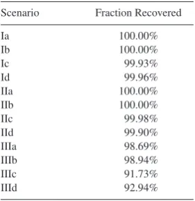
Table 1. Recovery of two-planet solutions. Scenario Fraction Recovered

Ia 100.00% Ib 100.00% Ic 99.93% Id 99.96% IIa 100.00% IIb 100.00% IIc 99.98% IId 99.90% IIIa 98.69% IIIb 98.94% IIIc 91.73% IIId 92.94%

epochs would generate six lists of 50-epoch samples, preserving the sampling characteristics of the real data. The result is 3871 lists of 50 observational epochs, each drawn from a real AAPS target and hence preserving all the associated idiosyncrasies of real data. Sets of 50 observation times for each of the 10 000 simulated data sets were then drawn at random (with replacement) from this pool. While the replacement means that some simulated data sets had identical observation times, we emphasize that the simulated velocity measurements are different, as described below.

2.2 Noise model

We simulated stellar velocity noise by choosing the radial velocity values and their uncertainties by a random draw from the AAPS data for six stable solar-type stars (531 epochs). These velocities have a

mean of zero and an rms scatter of 2.99 m s−1_{. In this way, we assume}

the input data are purely noise containing no planetary signals, and we have made no assumptions about the noise distribution (e.g. Gaussianity). The uncertainties, derived only from photon

statistics, have a mean of 1.1 m s−1_{. We then add 3 m s}−1_{of stellar}

jitter in quadrature to the individual measurement uncertainties. From our experience in least-squares fitting, this treatment reduces the possibility of the fitting routine getting stuck in local minima due to high-leverage points with small uncertainties. In the next subsection, we describe the process for generating the simulated Keplerian signals, which are added to the noise to produce the final simulated data.

2.3 Simulated planetary signals

For all simulated two-planet systems, the velocity amplitude K

for each planet was assigned a random value between 20 and

100 m s−1_{. This is largely arbitrary, but reflects values typical of}

securely detected radial velocity exoplanets. That is, the amplitudes are large enough to be unambiguously detectable in the presence of noise, yet small enough to remain in the planetary regime. Each scenario resulted in 10 000 synthetic radial velocity data sets.

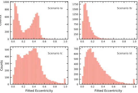
Scenario I– First, we considered a simple circular-double con-figuration, with orbits whose periods are in a 2:1 commensurability (Scenario Ia) at arbitrarily chosen periods of 100 and 200 d. In light of the observed pile up of planets at the 2.17:1 period ratio

(Steffen & Hwang2015), we repeated this with planets at periods

of 217 and 100 days, respectively (Scenario Ib).

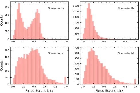
Scenario II– Next, we considered the combination of planets moving on slightly eccentric orbits. Scenario IIa consists of two

planets, both fixed ate =0.1, and at periods of 100 and 200 d

Figure 1. Distribution of fitted eccentricities for Scenario I (two circular planets).

as above. Likewise, Scenario IIb considers planets on periods of 217 and 100 d. For these eccentric orbits, we set the periastron

arguments atω1=0 andω2as a random value on [0, 2π]. Hence,

the relative apsidal alignment of the two planets is randomized.

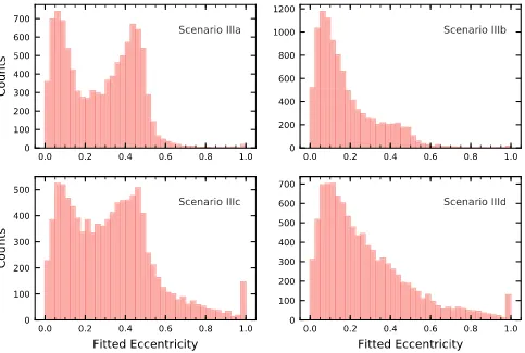
Scenario III– Finally, we investigated a more realistic choice of orbital periods for two circular planets. In Scenario IIIa, we drew the period of the outer planet at random (with replacement) from a set of 673 planets detected by radial velocity, obtained from the NASA Exoplanet Archive. The inner planet signal was then chosen to be exactly half this period. As above, Scenario IIIb sets the inner planet period such that the two are in a 2.17:1 period ratio.

For each of the three scenarios above, we also created ’c’ and ’d’ subsets. The ’c’ and ’d’ subsets of the above scenarios (I, II, and III) are analogous to the ’a’ and ’b’ setups (2:1 and 2.17:1 respectively), but using the more realistic observation epoch times drawn from real data as described in Section 2.1.

2.4 Orbit fitting

Armed with synthetic data sets, we proceeded to fit each with a

single Keplerian signal using the IDL packageRVLIN(Wright &

Howard2009), which employs the Levenberg–Marquardt method

for non-linearχ2_{-minimization. We obtained uncertainty estimates}

for the orbital parameters with the bootstrapping algorithm from the BOOTTRANpackage (Wang et al.2012). As pointed out by Wang

et al. (2012), we note that bootstrapping is not an ideal method to

determine parameter uncertainties in cases of sparsely sampled data, but our philosophy was to perform the fitting as blindly as possible. In order to save computational time, we limited our calculations

to 1000 bootstrap realizations; comparison of a small number of data sets for which we also obtained uncertainty estimates using 100 000 steps showed only marginal differences. The initial guess for the orbital period comes from the highest peak in a Lomb–

Scargle periodogram (Lomb1976; Scargle1982; Horne & Baliunas

1986), and we used a default initial value of 0.3 for the eccentricity.

We also employed an upper limit of 10 000 days for the orbital period. The only deviation from a completely blind fit we pursued

was to prevent the fitting routine from getting stuck at e = 0,

which sometimes happened especially if the fit was quite poor, and which we interpret as a peculiarity of the specific fitting package used. While not excluding circular orbits entirely, we automatically stepped through initial guesses of the periastron passage time if the initial fit returned an eccentricity of zero.

As a sanity check, we also attempted to fit each synthetic data set with a two-planet model, keeping the eccentricities fixed at either

zero or 0.1, depending on the scenarios described above. Table1

shows the degree to which this test successfully recovered the input periods of both planets to within 10 per cent.

3 R E S U LT S

Not surprisingly, the act of fitting a single planet to data containing two signals produced a wide range of results. In this work, we

are most concerned with the eccentricity; Figs. 1–3 show the

distributions of fitted eccentricities resulting from all scenarios. The primary aim of this work is to determine the frequency and conditions which cause two circular (or nearly-circular) planets to masquerade as a single eccentric planet in realistically sampled

Truly eccentric II

4233

Figure 2. Distribution of fitted eccentricities for Scenario II (Two slightly eccentric planets).

radial velocity data. To quantify this, we must first set some criteria for a ‘plausible” single-eccentric fit. As the input data consist of two Keplerian signals at two different periods, which we fit with a single planet, it is clear that a significant number of the resulting fits will be very poor. In defining ‘plausible” fit results, we must quantify what humans have been intuitively doing across three decades of radial velocity fitting. We therefore establish five criteria that must be passed for a given eccentric-planet fit to be deemed plausible.

(i) The fitted eccentricity must be at least 3σfrom zero.

(ii) The fitted velocity amplitudeKmust be at least four times

its own uncertainty:K/σK>4.0. This is derived from the NASA

Exoplanet Archive, in which 95 per cent of confirmed radial-velocity-detected planets satisfy this criterion.

(iii) The fitted velocity amplitude must be at least 1.23 times

larger than the rms scatter about the fit:K/rms>1.23. As above, we

choose this limit as that which holds true for 95 per cent of NASA Exoplanet Archive confirmed planets.

(iv) The fitted period must be less than 1.5 times the total duration of the observations. This is derived from noting that virtually no radial velocity planet discoveries are published with less than about 0.7 orbital cycles of observations (cf. fig. 4 of Wittenmyer et al.

(2011)).

(v) The rms of the fit must be less than three times the mean

measurement uncertainty: rms/σ <¯ 3.0.

While the final criterion is admittedly somewhat arbitrary, it eliminates obviously bad fits characterized by large residual scatter. Given that the input data always contain two signals, and we fit for only one, it is reasonable to expect a large number of instances in

whichRVLIN chooses one periodicity and arrives at a ‘best fit”

with an abominably large scatter.

Table 2briefly summarizes the plausible single-eccentric fits

resulting from the 12 trial scenarios described above, after applying these criteria. Scenario I, the double-circular configuration, resulted in 13.08 per cent plausible single-eccentric fits for the 2:1 period

ratio (P2=200 d), but none for the 2.17:1 period ratio. Increasing

the realism by drawing timestamps from real observations produced 19.04 per cent and 4.94 per cent such plausible fits for the 2:1 and 2.17:1 period ratios, respectively. Similar results were achieved in

Scenario II, using the ‘slightly eccentric”e=0.1 configuration.

Scenario III, where the outer periodP2was drawn from the set of

real planets, yielded the largest number of plausible single-eccentric fits, with 15.27 per cent (IIIa), 2.89 per cent (IIIb), 20.49 per cent (IIIc), and 9.30 per cent (IIId). The detailed characteristics of these plausible fits are discussed further in the next subsection.

3.1 Plausible eccentric single solutions

In this subsection, we investigate the properties of the plausible

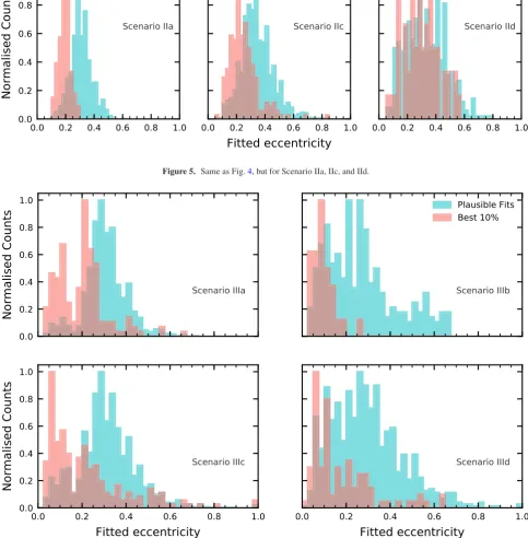
single-eccentric fits in more detail. Figs. 4–6 show as green

histograms the distribution of fitted eccentricities obtained by the RVLIN single-planet fits which passed all five criteria described above. Overplotted as red histograms are the ‘best” 10 per cent of plausible fits, those with the smallest ratio of rms scatter to mean measurement uncertainty. This selection resulted in fits with rms

values of 2.9-5.1 m s−1_{(where the mean measurement uncertainty}

is∼3.2 m s−1_{). These are fits which are most likely to convince the}

Figure 3. Distribution of fitted eccentricities for Scenario III (two circular planets with ’realistic’ orbital periods).

Figure 4. Distribution of fitted eccentricities for the ‘plausible” single-eccentric fits found in Scenario Ia, Ic, and Id.

observer that a single eccentric planet is a good fit to the data, when in reality two planetary signals are ensconced within.

In Scenario I (periods fixed at 200:100 or 217:100 d), the bulk of the best fits were generally restricted to eccentricities between

0.2 and 0.4, with a handful of examples out toe ∼ 0.6 for Ic

and Id, which sampled the simulated velocities using time series from real stars. Notably, the 2.17:1 arrangement (Scenario Ib; no histogram possible) never produced a reasonable single-eccentric

solution. Scenario II, in which slightly eccentric (e= 0.1) pairs

of input planets were tested, gave very similar results to Scenario I. Scenario III was the most realistic, with periods drawn from real radial velocity planets, and resulted in the highest fraction of plausible single-eccentric fits. As in the previous trials, the best fits

clustered at lower eccentricities (e<0.2) but developed a long tail

extending even toe>0.9 for Scenarios IIIc and IIId (Fig.6). Closer

inspection revealed that the extreme examples were characterized by pathologies such as (1) reaching the maximum allowed period (10 000 d) with an error bar of more than 200 per cent, or (2)

Truly eccentric II

4235

Figure 5. Same as Fig.4, but for Scenario IIa, IIc, and IId.

Figure 6. Same as Fig.4, but for Scenario IIIa, IIIb, IIIc, and IIId.

amplitudesK> 500 m s−1_{with large uncertainties, likely driven}

by phase gaps in the time series (as the observation times were taken from real data). These ‘best” fits were selected strictly by the lowest rms scatter, with no human intervention as yet, and so such oddities are to be expected. We explore the cause of these peculiarities further in the next section.

Fig. 7shows an example of a simulated data set that yielded

a ‘good” single-eccentric fit, with e = 0.31 ± 0.03, K =

95.6±0.9 m s−1_{, and an rms of 2.56 m s}−1_.

4 D I S C U S S I O N A N D C O N C L U S I O N S

In this work, we consider the problematical false positive single-planet solutions that can arise from poorly sampled radial velocity observations of systems containing two exoplanets moving on near-circular orbits. With poor sampling and noisy data, the analysis of such systems can often return a convincing single-planet solution, with that planet moving on an orbit with moderate eccentricity. It is likely that a number of such near-circular exoplanetary

Figure 7. Example of a simulated data set for which the circular-double combination can be plausibly fit with a single eccentric model. Shown is an example from Scenario IIId, chosen from the ‘best” 10 per cent subset, to illustrate the pathology we investigate here. This fit has a period of 548.8 days,e=0.31±0.03, and an rms of 2.56 m s−1. The true injected data are two circular orbits with periods of 580.7 and 267.6 days.

couplets remain undiscovered among the many ’confirmed’ single, moderately eccentric exoplanets.

The results of our analysis demonstrate the range of eccentricities for which it is conceivable that a circular two-planet system can masquerade as an eccentric single planet. Particularly for the most realistic trials (IIIc and IIId), there was no obvious cutoff eccentricity beyond which circular-double systems failed to produce plausible single-eccentric fits. However, in reality, it seems reasonable to expect such a threshold to exist. This is due to the shape of the radial velocity orbit departing so far from sinusoidal that it realistically cannot be reproduced by only two circular components, which is the problem at the heart of this degeneracy (as noted in

equation (1) of Boisvert et al.2018). We see evidence of such a

limit for the ’a’ and ’b’ subsets, in which the sampling turned out to be less realistic than for the ‘c’ and ‘d’ scenarios.

The grand mean-fitted eccentricity across all scenarios (Table2)

ise=0.32±0.12, with a 95 per cent confidence interval of [0.09,

0.59]. We take this to be the ‘sweet spot” (or danger zone) for deceptive configurations. If we consider only the ‘best” 10 per cent

of the plausible single-eccentric fits, we derive a grand meane=

0.23±0.12, with a 95 per cent confidence interval of [0.05, 0.53].

Table 2. ‘Plausible” single-eccentric fit results from 10 000 trials.

Scenario Number Mean eccentricity

Ia 1308 0.31±0.06

Ib 0 –

Ic 1904 0.35±0.11

Id 494 0.32±0.15

IIa 1238 0.31±0.07

IIb 0 –

IIc 2004 0.35±0.11

IId 548 0.33±0.14

IIIa 1527 0.31±0.10

IIIb 289 0.28±0.16

IIIc 2049 0.31±0.13

IIId 930 0.29±0.16

Our results therefore show that more eccentric planet candidates (e

0.5) are exceedingly unlikely to be mimics due to this degeneracy.

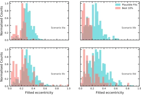
As noted above, the best such fits (in an rms sense) sometimes exhibited pathologies such as extreme amplitudes brought on by phase gaps, or fitted periods at the upper boundary and with outsized error bars. In Scenario III, up to 9 per cent of trials failed even to recover the two injected planets when subjected to a proper

double-Keplerian fit (Table1). We repeated the five tests described

in Section 3 for the subset of trials which passed the sanity checking (see Section 2.4). We show the results for this new set of ‘plausible’

results in Fig. 8. For Scenarios IIIc and IIId, which were most

affected, we indeed see that all but 2–3 of the e > 0.6 fits are

eliminated. A handful remain, but the vast majority of ‘good’

single-eccentric fits havee0.4. This is again consistent with our result

that the ‘danger zone’ lies generally in the range betweene∼0.2

ande∼0.4.

The results presented herein are also relevant to exoplanet searches that utilize the transit method. The relative lack of orbital phase coverage from transiting planets without accompanying RV data makes the reliable extraction of orbital eccentricity from transit

light curves a challenging endeavour (e.g. Kipping 2008; Van

Eylen & Albrecht 2015). Statistical studies of orbital

eccentrici-ties derived from Keplerdiscoveries have found the eccentricity

distribution of transiting planets to be consistent with that from

the RV exoplanet population (Kane et al. 2012). It was further

concluded by Kane et al. (2012) and later by Van Eylen & Albrecht

(2015) that there is a negative correlation of orbital eccentricity with

planet size, particularly for those planets in compact systems. These factors underline both the need for complementary RV observations of transiting planets to reliably extract orbital eccentricities, and the potential degeneracy of circular orbits in the terrestrial regime. Ex-oplanet discoveries from the Transiting ExEx-oplanet Survey Satellite

(TESS) are expected to primarily be in relation to relatively bright

host stars where such a complement of precision photometry and

RV data will be far more accessible than for theKeplersystems

(Ricker et al.2015). In particular, extended mission scenarios for

theTESSmission, such as those described by Sullivan et al. (2015),

allow for the detection of longer period planets that will be more likely to have larger eccentricities.

Through the course of this work, we have demonstrated the impact of poor sampling on the veracity of convincing radial velocity exoplanet detections. Our work reveals the regime for which most caution should be exercised when considering whether a single-planet fit to observational data is a reflection of the true reality of the system in question. At the same time, however, our results add credibility to the detections of exoplanets moving on

highly eccentric orbits, such as HD 80606b (e= 0.933±0.001;

Wittenmyer et al.2007), HD 4113b (e= 0.903± 0.005; Tamuz

et al. 2008) and HD 76920b (e = 0.856 ± 0.009; Wittenmyer

et al.2017b). While such planets are clearly oddities, our results

suggest that they are not false-positive, ghost planets. Indeed, our results suggest that deceptive planetary couplets will rarely, if ever, masquerade as single planets with orbital eccentricities greater than

e∼ 0.6, consistent with the results of K¨urster et al. (2015) as shown

in their fig. 4.

In future work, we intend to extend this analysis still further, examining a wider range of planetary couplet period ratios, orbital eccentricities, and masses. In addition, it is interesting to consider whether similar effects would result from deceptive triplets or quadruplets – in other words, whether it might be possible to mimic a signal of arbitrarily large eccentricity through the superposition

Truly eccentric II

4237

Figure 8. Same as Fig.6, but with the failed data sets excluded.

of a given number (N>2) of signals resulting from planets moving

on near-circular orbits.

AC K N OW L E D G E M E N T S

CB is supported by Australian Research Council Discovery Grant DP170103491. JC is supported by an Australian Government Research Training Program (RTP) Scholarship. This research has made use of NASA’s Astrophysics Data System (ADS), and the SIMBAD database, operated at CDS, Strasbourg, France. This research has made use of the NASA Exoplanet Archive, which is operated by the California Institute of Technology, under contract with the National Aeronautics and Space Administration under the Exoplanet Exploration Program.

R E F E R E N C E S

Anglada-Escud´e G., L´opez-Morales M., Chambers J. E., 2010,ApJ, 709, 168

Boisvert J. H., Nelson B. E., Steffen J. H., 2018,MNRAS, 480, 2846 Butler R. P., Marcy G. W., Williams E., Hauser H., Shirts P., 1997,ApJ,

474, L115

Campbell B., Walker G. A. H., Yang S., 1988,ApJ, 331, 902 Carter B. D., Butler R. P., Tinney C. G. et al., 2003,ApJ, 593, L43 Fischer D. A., Anglada-Escude G., Arriagada P. et al., 2016,PASP, 128,

066001

Gillon M., Triaud A. H. M. J., Demory B.-O. et al., 2017,Nature, 542, 456 Hellier C., Anderson D. R., Collier-Cameron A. et al., 2011,ApJ, 730, L31 Horne J. H., Baliunas S. L., 1986,ApJ, 302, 757

Jones H. R. A., Butler R. P., Tinney C. G. et al., 2006,MNRAS, 369, 249 Kane S. R., Ciardi D. R., Gelino D. M., von Braun K., 2012,MNRAS, 425,

757

Kipping D. M., 2008,MNRAS, 389, 1383

K¨urster M., Trifonov T., Reffert S., Kostogryz N. M., Rodler F., 2015, A&A, 577, A103

Latham D. W., Mazeh T., Stefanik R. P., Mayor M., Burki G., 1989,Nature, 339, 38

Lomb N. R., 1976,Ap&SS, 39, 447

MacDonald M. G., Ragozzine D., Fabrycky D. C. et al., 2016,AJ, 152, 105 Marmier M., S´egransan D., Udry S. et al., 2013, A&A, 551, A90 Mayor M., Queloz D., 1995,Nature, 378, 355

O’Toole S. J., Jones H. R. A., Tinney C. G. et al., 2009,ApJ, 701, 1732 Ricker G. R., Winn J. N., Vanderspek R. et al., 2015, JATIS, 1, 014003 Robertson P., Horner J., Wittenmyer R. A. et al., 2012,ApJ, 754, 50 Scargle J. D., 1982,ApJ, 263, 835

Steffen J. H., Hwang J. A., 2015,MNRAS, 448, 1956

Sullivan P. W., Winn J. N., Berta-Thompson Z. K. et al., 2015,ApJ, 809, 77 Tamuz O., S´egransan D., Udry S. et al., 2008, A&A, 480, L33

Tinney C. G., Butler R. P., Jones H. R. A. et al., 2011,ApJ, 727, 103 Trifonov T., K¨urster M., Zechmeister M. et al., 2017, A&A, 602, L8 Van Eylen V., Albrecht S., 2015,ApJ, 808, 126

Wang S. X., Wright J. T., Cochran W. et al., 2012,ApJ, 761, 46

Wittenmyer R. A., Endl M., Cochran W. D., Levison H. F., 2007,AJ, 134, 1276

Wittenmyer R. A., Tinney C. G., O’Toole S. J. et al., 2011,ApJ, 727, 102 Wittenmyer R. A., Horner J., Tuomi M. et al., 2012a,ApJ, 753, 169 Wittenmyer R. A., Horner J., Tinney C. G., 2012b,ApJ, 761, 165 Wittenmyer R. A., Tinney C. G., Horner J. et al., 2013a,PASP, 125, 351 Wittenmyer R. A., Wang S., Horner J. et al., 2013b,ApJS, 208, 2

Wittenmyer R. A., Johnson J. A., Butler R. P. et al., 2016a,ApJ, 818, 35 Wittenmyer R. A., Butler R. P., Tinney C. G. et al., 2016b,ApJ, 819, 28 Wittenmyer R. A., Horner J., Mengel M. W. et al., 2017a,AJ, 153, 167 Wittenmyer R. A., Jones M. I., Horner J. et al., 2017b,AJ, 154, 274 Wolszczan A., Frail D. A., 1992,Nature, 355, 145

Wright J. T., Howard A. W., 2009,ApJS, 182, 205

Wright J. T., Marcy G. W., Howard A. W. et al., 2012,ApJ, 753, 160

This paper has been typeset from a TEX/LA_{TEX file prepared by the author.}