The quantum electrodynamics of a medium

(1)

The.l. by

Harold Thoma. Yura

In Partial Fulfillment of the Requirement. For the Degl'e. of

Doctor of PhUoaophy

California Institute of Technology Paaadena, California

(2)

(3)

By uoine the Fcyrunan diagram technique, a unified analyoh ia given of the Qunntum Electrodynamics of a Medium. We consider both an atomic medium and an electron ga.. The photon propagator in a medium i8 calculated by summing the mo.t highly divergent diagrams in each term of the perturbation series expansion of the photon propa-gator. An explicit form for the interaction amplitude of two arbitrary currents in a medium is given. From this amplitude a complete com-ple:, dielectric function ir.J defined (at the pole of a photon propagator).

Furthermore, we h~ve examined the photon propagator for ita poles in order to obtain dispersion relatione which yield the energy-momen-tum relation for free motion of the system. We have considered, in detail, an atomic oystem and an electron gas. In both casea explicit dispersion relations are found over a wide range of energy and momen-tum variables. Effect. of finite temperatures are discussed. Also we have obtained the energy 10138 of fast incident charged particles passing through an atomic medium from the seli energy of the incident particle

,

in the medium. The energy loss so obtained consists of three parts:

lOGS due to excitation of atoms, loss due to ionization of atoma, and a Cel"enkov loss. General features of the energy 10 •• are dhcu •• ed.

(4)

PART I

n

IU IV V INTRODUCTION

PHOTO~{ PROPAGATION IN A MEDIUM AND THE INDEX OF REF ACTION

A. Quclitative Features of the Photon Pl'opagator

PAGE 1

4

in a Medium 4

B. Calculation of the Photon Propagator in a

Medium 6

C. General Expression for ~~vl 11

D. Calculation of

i3..,.v

in the Cale of Small K 13 E. Current-Current Interaction. in a Medium in

the Caee of Small K 23

F. Index

of

Refraction of a Medium 29 G. DiscuBsion of the Index of Refraction 31 H. Calculation of

f3..,.v

in the Case of Large K 33 I. r.urrcnt-Current Intaraction in the Ca8e of

Large.K 35

J. Real Processes in a Medium: Pole. of the '

Photon Propagator 36

ENERGY LOSS OF RELATIVISTIC CHARGED

PARTICLES IN A MEDIUM 56

A. Relation to Looo 56

B. Self Energy and Decay Rate of a Particle in

a Medium 58

C. On the Evaluation of the Integral F R (w) 66 D. ( h the Evaluation of the Integral F S(w) 70 E. General Expresoions for the EnoriY LOll 84

SOME MISCELLANEOUS TOPICS 95

A. Effect of Finite Temperature. on the Photon

Propagator for Small K 95

B. Damping 100

SUMMARY AND CONCLUSIONS APPENDIX .A

APPENDIX B REFERENCES

109

111

(5)

I. INTRODUCTION

The purpose of this paper is to give a unified treatment of the Quantum Electrodynamics of a Medium. By the Quantum Electrody-namics of a Medium we mean the quantum mechanica of a aystem of charged particle. (medium) interacting with the electromagnetic field (i. e., acalar.longitudinal and transverae photons). For the .mo~t part we will be dealing with an atomic medium (i. e., a medium consiating of atoms interacting with the electromagnetic field).

There are a n~ber of physical problema of interest that ar18e in connection with the interacting system (medium plua photon field). For example; the propagation of photona through the medium (index of refraction), the normal modes of the interacting system, the energy loss of fast charged particles passing through the medium, etc. are typical problems. In the past these problema have been 8tudied mainly from a classical point of view. For example, the energy 1088 problem

•

was first treated by N. Bohr in 1915 using cla8sical technique8. Many people have since extended Bohr'o classical treatment.

It was not until 1956 that Tidman (1) gave a non-phenomenologi-cal quantum mechaninon-phenomenologi-cal treatment of the energy loss that included the contribution to the loss from large impact parameters (or equivalently small momentum transfers). It is in thia region of large impact param-eters where it 10 necessary to include the pa8sive effects of the medium on the energy 108s. Tidrnan uses the hamiltonian approach, that ie, the

•

(6)

approach described in Hoitlel°'s book (2). This approach necessitates the use o{ a nwnbor of approximations (e. g., that the Coulomb inter-action in the medium does not differ from that in vacuwn). Since

Tidman'& treatment of the atoms of the medium 18 non-relativistic, his results are applicable only to small momentum tranders. Further-more, Tidman makes the approximation that the dielectric function (the square of the index of refraction) is real. None o{ these approxima-tions are necessary in the method used here, the Feynman diagram technique. By this method the problem may be treated in a completely four-dimensional fashion, and it follows that the result. are valid for all value. of the momentum transfer. Another consequence of our {our-dimensional formalism 18 the general validity and \I.efulne •• of the cur-rent conservation law (e. g., this law enables \18 to derive the modifica-tion due to the medium of the coulomb interaction). Finally we are able to obtain the complete complex dielectric function for both large and small momentum transfers. The relation between the imaginary part

of the dielectric function and the energy 108s of fast charged particles

is derived.

In addition we have appUed theae methods to a consideration of the normal modes of the system consisting of the atomic medium to-gether with the electromagnetic field. By a simple extension of the ••

methods, we arc able to derive the complete relativiatic dispersion relation {or the electron gas,· a relation which reduc •• in the non-relativistic approximation to that o{ Bohm and Pines (3).

(7)

(8)

II. PHOTON PROPAGATION IN A MEDIUM AND THE INDEX OF REFRACTION

A. Qualitative Features of the Photon Propagator in a Medium

In the following we are u8ing gaussian unit. with " • c II

h

then eZ

~

1/137. Four-vectors will be denoted by .ma1l1etter. [e. g., k II (w,

K)].

The dot product of two four a, b b taken a. a· b • atb

t - -;.

b.

Ais 0, the notation

<t

I I at''' t - -;. -:; is us ed.

In thie section we will discua. the photon propagator in a medium.

The follo .. ·ring assumptions are made in this paper. The medium is a.-sumed to be nonconductive and to consist of N identical, infinitely heavy, nonpolar, nonmagnetic, randomly Ilituated a.toma per cubic

,

centimeter. We take N to be small enough ao that we may neglect any direct interaction between atoma of the medium. We a.sume that the intrinsic properties of the atom a of the medium are known, that h, the energy eigenfunctions ~n' energy eigenvalues ' En' and line widths '\' are assumed known. Also, for simplicity, we will conaider one

n

electron atomB. We take the temperature of the medium to be so low that in the ground state of the medium each atom ia in it. ground state. In Chapter

IV

we will discuss the effects of a finite temperature on the photon propagator.

In order to obtain tho photon propagator in a medium we proceed as follows. Conoider two current sourcea in tho medium. One current, J("].) , is at an arbitrary space-time point 1; the other, J'(x_Z

>'

at an arbitrary space-time point 2.

(9)

Let us usk for the probability amplitude that the current at point 1 emit. a photon, the photon propagating through the medium from point 1 to point Z suboequcntly being absorbed by the current at point 2. Let U8 call this amplitude

A.

We write

A

in the following manner

•

ike

x,.

• •

-lk·

x

₂

Writing J~(:;) a

J

~e (emits) and J,,(x₂) a J~e (ab8orbs) we have

(n-l)

Now, due to the homogeneity of the medium P ~,,(:;,

xz)

mU8t be a function only of the dif~erence

1x,.-xzl.

Therefore

'. , "

/k

z

•

For the vacuum

"11"

is just

-4"

6.,.".

With a medium present

TI..,."

will differ from the v~cuum case. It will contain the effect of the medium

on the propagation properties of the photon. In the rest of this chapter we will concentrate on calculating the" propagator"

"f1".

Physically we would expect that if the spatial separation between points ,1 and Z is larger than the mean separation between the atoms of

the medium. which we take to be of the order of the Bohr radiua, tho '· 0 • +1 if f1

= " =

4. a -1 if f1

= " •

1, Z. 3 and zero otherwise.

(10)

effect of the medium will be to modify the propagation properties of the p:~::>ton from the case of propagation in vacuum. The atoms of the

medium will pacoivcly scatter the photons; for example, there is a finite probability that the following process will occur: A photon of momentum l~ excites an atom of the medium to a virtual exdted state, the excited atom then decays re-emitting a photon of momentum k. On the other hand, for a spatial separation that b smaller than the

separa-tion between atoms of the medium we expect that the atom. will have

little effect on the photon propagator for vacuum.

B. Calculation of the Photon Propagator in a Medium

The coupling between electrically charged particles and the electromagnetic field is characterized by the dimensionless constant e2 Il:S 1/137. BecaUfle this constant is much les8 than one the usual method of computing amplitudes in quantum electrodynamics ia to use perturbation theory (expanding the amplitude in a power series in (2).

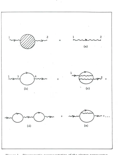
This is the method that is uced here. In order to calculate the contri-butions to the amplitudes in perturbation theory we use the Feynman diagram technique. The utility in using Feynman diagrams is that the cont:..-ibution from each term in the perturbation expansion can be written dOVIn by inopec~ion. Figure 1 shows some of the lower order diagrams aflGociatcd with "fJ.v. Diagram la represents the propagation of a

(11)

1 2

=

1 3

+

(b)

(d)

1

+

1 2

~

(a)

(c)

1-=:- + •••

[image:11.612.115.566.52.644.2]

(e)

(12)

photon interacts with an atom of the medium causing the atom to make a transition to an excited state. From 3 to 4 we have an atom in a virtual excited state. We represent this by

30

4 • At 4 the atom de-excites, emitting a photon (of momentum k) which propagate. freely from 4 to 2. Diagram lc differs from diagram lb only in that the photon that arrives at 2 is emitted before the photon coming from 1 is absorbed. Diagram la, lb, lc represent the complete 2nd order (in e) contribution to the photon propagator in a medium. Diagram.ld. 1e aro part of the

fourth order expansions for "J1v'

To second order P lI-_v is given by.

P

= _ . 4w

[(2Tl)4₆4(k -k')6 .:fa p(2) ] •

J1v k 2

+ i~

lI-" lI-v (U-2)

(2) . 4 4 • (2) (2) / • 2

where P J.lv is of the form (21T) 6 (k - k )~ J1v' In 11-2, P J.lv is -411" (k ) times the amplitude per unit volume that a photon of polarization JJ.. momentum k excites an atom of the medium to an axcited state with the atom aubsequenUy emitting a photon of momentum

k',

polarization

/ • 2

v plus -411' (k) times the amplitude per un~t volume that a photon of polarization v, momentum. k' is emitted by an atom of the medium, the atom being raiGed to a virtual excited state with the atom subsequently de-exciting by absorbing a photon of polarization JJ., momentum. k.

Diagrams la, lb, 1c are the complete contribution to the photon propagator to second order. In the fourth order there are two 'kinds of

diagramo that contribute: iterations of aecol'ld order diagrams (see for

(13)

example figure ld) and new types of diagrams that cannot be obtained

from iterating second order diagrams (figure Ie shows a typical

dia-gram of this type). Let us call a diagram as proper if it cannot

be reduced to two simpler diagrams by cutting a I ingle photon line.

ThUB, in figure 1, (b) and (c) are proper .econd order diagrams and

(e) is an example of a proper fourth order diagram while (d) 18 not a ·

proper diagram. In the n'th order of perturbatiqn theory we get

con-tributions from n'th order proper diagrams plus concon-tributions from

iterations 01 lower order proper diagrams.

Call

tl~~

the sum of all the proper diagrams of the n'tn order.

Then the total amplitude for the medium to ab80rb a photon of momentum

k, polarization ~ and the medium subsequently re-emitting a photon of

momentum k polarization

v

is given by [ omitting the factor

(Z1r)4 64(k_k')]

(n-3a)

(n-3b)

That is, 11 is proportional to the inverse of the matrix (6_tl(Z) _tl(4) - ••• )

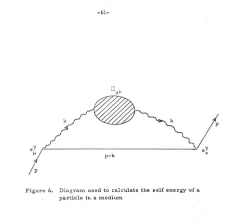
which just involves proper diagramo. What we are doing in calculating

"~v is essentially calculating the self ener3Y of a virtual photon in a

medium due to virtual interaction. with particle. of the medium. The

(14)

photon propagator at w

=

K (vacuum case) to somewhere else. That is, the inf'nite series n-3a is a perturbation expansion calculation of

2

this shift of the pole. Since e is 80 omall we expect that the location

of the 1-ole will be close to w

=

K and also that the nature of the pole wiU

be the same as the vacuum case (e. g., a .imple pole). We note that

each successive term in 11-3a is getting more and mOl'~ divergent near

w

=

K. Now

~Z

contains a factor eZ jk2,

~(4)

a factor 02(e 2 jkZ) etc.

So, for example, in the fourth order we get two terms,

~

(4) and

(l:~(Z»Z.

Both of these terms are of order e 4 but nea'r- w. K,

(~(Z»Z,

the iterated second order term, dominates the

~

(4) term because of

the extra factor l/kZ• It b easily seen that th18 will be true to all

orders (1. e., the iterated second order term will be dominant near

w

=

K). The expression U-3b is telling us that the location of the new

pole will be determined where the matrix

k2(6_~(2)_~(4)_

••• ) -1 18

singular. .Physically, at the pole, we obtain the relation (diapersion relation) between w (energy) and K (momentum) for real processes

in a medium. Aa an approximation to n-3b we take the expression

(n-4)

This expression hi the sum of the n'lost highly divergent terms of the

perturbation expansion n-3a in each order. W. shall .ee that we do

(15)

c.

GENERAL EXPRESSION FOR ~ v !J.

Applying the Feynman rules (4) to diagrams Ib and Ic we get

where

I

signifies the sum over all the atoms in a unit volume, . ~ i

(n-6)

i - i _ -iE t

llt (x)

=

tp (,t)e n are the stationary solutions for the ith atomic

n n

electron (i. e., the wnts are the solution of

(iV"~

eJj.ExT - m)w a 0,

S •

3- ExT .

normalized to <p fP d x :I 1, where A is the external field actmg

on the electron i. e., th~ coulomb field of tho nucleus), the quantities

'-' _{, J.&.} (~= x, y, z, t) are the familiar gamma matrices which satisfy _.

V'tl-:_Vv

+

'Iv'l..,. :: 20J.&.v' and

Vi

is the adjoint of

W

( .

\)+"

t). The first

term of U-S corresponds to diagram Ib and the second term to

dia-gram lc.

After inserting II-6 into II .. S and combinina terms we get:

(16)

p

=

J.LV

Z i4 Tie

(kf)2

+

terms with k;: -k' for t

4

>

t3

• Ii •

-I

.

..

(U-7)

Consider the atomic matrix elements in 1I-7. For bound state the

wave functions (,On are non-zero for values of I'~

I

up to the order

of the Bohr radius a_o• So for small K (Ka

o

«

1) we can expand the

--...

....

iK·x - iK.x

-exponential factor e a8 series of powers of K: e .. l+iK· x II

1

+

iKz. we choose a coordinate system with the z axis along the · ...

ec

-tor K. Also in this region of K we make the nonre1ativistic

approxi-mation in the treatment of the atomic electrons. Physically in this

region of K the atom receives a momentum which is small compared

with the original intrinsic momentum (meZ) of the atomic electrons.

On the other hand in the opposite limit, that of large K (Ka_o

»

1),

it is evident physically that we can regard the atomic electrons a8

free. and at rest (atom receives a momentum which is large compared

to meZ). This can also be seen from the atomic matrix elements in

II-? For large K. the integrand contains a rapidly oscillating factor

eiK• x. and the integral is almost zero if (,On does not contain a similar

factor. Such a function ~n corresponds to an ionized atom with the

(17)

con

-servation of xnoxncntum between the incident photon (K) and the original

xnoxnenturn of the electron (which is much smaller than

K).

D. CALCULA TION OF (3 IN THE CASE OF SMALL K J.1V

where £ is to approach zero through positive values after the

n

integration has been done. Upon inserting II-S into U.S and

rear-•

ranging te rms we get,

x 1

+

terms with k;::.k'

E

(l-ic;)

+

D

n

Performing the integralo over tl and t2 we get,

4 2

I{SOO

tS

3

-iK'.~

j

p • - ~ (211') 6(w-w I) dO 6(O+E iw) d);'.,"i e 'V fP i

*"'"

(k')'"" '-' -0:) 0 ~ 0 "

i, n

· In the following the dummy integration variables will be denoted by the

(18)

(11-9)

To proceed further, we first examine the contribution from

positive energy states. In II-9 for a given atom (i) the (1,i iii q1 (-; - -:i)

n

-where a

i is the position of the i'th nucleus. So if we write, say,

as

and similarly for the other terms then this form haa the integration

variable centered around the i'th nucleus. Since all of the atoms are

identical the atomic matrix elemente for different 1 are equal: the only

-

---ia_l • (K-K')

dependence on i in II-9 will appear in a factor e Q Then

-

--~

e-ai • (K-K )

S

3- -1-;·

(K-K")

L

-

N d ae

i

(19)

I

-iKe

x

I

iKe

x

I

4 2N 4 4 ' \ { < 0 e 'I n> < n 'I e O >

P

=

-

1'I'c

2 (2tr) 0 (k-k )

6

v J.1

J.1 v k all n En (1 -

id -

Eo - w

4 4

:I (211') 6 (k - k')~ JJ.V

(n-10a)

(U.10b)

where <nl'l

ei

K

·~IO>.

Sd~

'I

eiK

.

~".

Consic1er the atomic

JJ.

n....

0

matrix element

where ....

=

(t, x, y. z).

In the nonrelativiotic ap~roximation

a....

become.,

a~

.

;

<nl'lt(l

+

Uu)10>

=

(1

+

iKz)no

=

iKz _no

(D-11)

whe

re

zno

=

S

cp: Z CPo d3-;; (the matrix element of 1 between n anc1 0

vanbh because thooe states are orthogonal to each othel"). Aho

a _x~ <nl'l 10> _x

J

3 -

+

1:1 c1 xcp 0. cp

n x 0

=

_{x no '}

(20)

-

-(since in the nonrelativistic approximation (1 is replaced by

x )

similarly'

=

i(E - E )x

n 0 no

:= iw x no no

Also for a given value of En there b a aum over the angular

momen-..

tum statea of the atom. As is well known in the dipole approximation

111. 1:1 :t: 1. Since the ground state of the atom is an a state the excited

states must be p states. So for a given En there are three angular

momentum states (m.t 1:1 0, II: 1). Now it 1s easy to aee that within the

dipole approximation that the only non-zero terma of ~

'"'v

are: f$ll'

l3

_ZZ' 13_{33 ,} 13_34, j3 43' and 13_44, where the lndices " corresponda to t,

-3 to z (th~ direction of K). 1 and 2 to " . and ,,_ respectively

(-:;.,iy

'-

,

'

.

Xi!Y

'-

).

The reason or this £ is the following: consider, for example.

13

13• Physically we are asking for the amplitude, in the

di-pole approximation, that an atom absorbs a right-handed polarized

photon and emits a longitudinal photon. Now for a atven value of En

where the :t: 1 and 0 correspond to excited states with m_t II d: 1 and 0

(21)

(I respectively. So

--since. for example. a₃(+)

=

altO) a a

1(-) a O. Similarly, all oif

di-agonal elements except ~34 and ~ 43 are zero. Now con.lder the

diagonal terms

Also

and

also

There!or~ from II-lO and II-12 we obtain that the contributions from

the sum over positive energy states is given by

, 2

13

8 trN e \:' ' Z

I

J Z ( 1

+

1 ) 11

=

22

=

33 a • k2 ~ wno "no W -w w iw

n+ no no

(n-13a)

*

:t:icb iOf

q1n(:!:'O) contain a iactor ,oi e and e :respectively.

,I

(See (2-11) ).

**~ Henceforth zno

1 12

denotes the dipole matrix element summed over

(22)

(ll-13b)

Now in the dipole approximation we calculate the contribution

from negative energy states. For a negative energy state En- - (m

+

Order Rydberg). Now Eo - m

+

Order Rydberg so En-Eo'" - 2m

+

O(Ryd.). So £0 r (a) much less than m we get, from

n-9,

that the

contribution to say

P

u

(a ~22111 ~33) becomes (neglecting terms 01

order Ryd./ m)

n-• -

~

L

<olYlP In><nly1IO>

alln

I: -

~

<oIYl,D

'V1 JO

>

(D-14)

where

P

is the projection operator lor negative energy states (i. e.,

P

In +> I: 0,

P

In -> • In

->.

Neglecting terms of the order Ryd./m

P

can be taken to be:

(D-15)

Substituting 0-15 into II-14 we obtain

1

(0-16)

-

-II-16 can be recognized as the contribution lrom the A2 term in the

(23)

The contribution to

l3

44 from negative energy states is

, 1

I1u

1 (y t -1)

j3 44 - -

m

<

0 1 Y 4("/ , 410

>

D -

in

<

0 J Y t

--z

'V t J 0

>

D 0

Also. the contributions to all off diagonal element. are zero. For

exaxnple

DO

Abo

=

0

since 'V t J 0>::1 J 0> •

Summing II-16 over all of the atoms per unit volume gives a

factor N. That is (replacing all the factors) the nOn-zero contribution

from negative energy states per unit vohune b.

Z

411'e , N)

J3

_{U ::}

l3

_ZZ

=

J3

₃₃II

--z

,-

iii

k

(U-16')

, From II-13 and II-16' we get that the contribution to

IS

from both

(24)

(II-l?b)

We remarlt that the expression II-I? could have been written down by

inspection. Consider. say ~ll. Thill i8 the amplitude for transverse

waves propagating exciting-de-exciting atoma. Treating the atomic

electrons as 1'lonrelativiotic the amplitude for diagrams lb. lc can be

obtained as follows: Amplitude for propagation from 1 to 3. _4,,/k2.

amplitude for a transverse photon to excite atom to nth state.

iew

z

.

~·

The amplitude for the system to propagate in the inter-no inter-no

mediate state 3-4 is l/(E. - Ei _'_in _nt)' where E. h the initial energy 111

of the system Oust prior to 3) and E

int ia the energy of the system

in the intermediate state. For both daigrams Ein iii Eo

+

w. For Ib,

Ei t

=

E and for lc, Ei ... iii E

+

2w. Amplitude for the photon to be

n n n~ n

+

emitted by the atom -iew _{no no}z • Amplitude to propagate from 4 to 2.

_ 4"jk2 •

Also in the nonrelativistic approximation there is a contribution,

2/

-for transverse waves only. from the e m (A • A) term in the

hamil-tonian. Thie term contributes, per atom, an amount e 2

1m.

Putting

everything together and holding back one of thCl factors 01. -4w/k2 we

get

9Henceforth we write

I

as

2:.

n+

n

..

'

(25)

R 4 ";ie N

~

I ( .

+ )

I 1

+

1 ) (i ') ]

+

1 }

... 11= - k2

10

L

-lW_noZno\w+E

-E

w+E

-2w-E

WnoZ no

iii

o n 0

n

T: s i j\\S~ II-17a. (To get the contribution per unit volume we just

multiplied by N since the atoms do not interact with each other.) To

get ~ 44 we note that for · coulomb; ~ photons there 18 no contribution

.-

-from the A • A term hence there 18 no factor of

11m,

and the atomic

matrix elements are - Kzno.

411'Ne2 '\' K21 121 1

::

2-

~ zno \ w -w

k . _n no

which is just II-17b. The expressions -,II-17 may be simplified by

making use of the Thomas Reiche awn rule (S) which say. that

L

2

•

f _no::

2

2mw _noJz _no

I •

1

n n

or

1

:: 22:

C&)no

1z

nol2 (n-1S)

m

n

Substituting II-IS into n-17a we obtain

• . 2

(26)

and from II-13

2 1{2

I

J

12

~44 • 8"Ne ~ _k' w _{no no}z .

n

1

Z 2

w _no-w

1

2

Z

w -w

no

- 2)

(11-19)

(II-20a)

(II-20b)

The expressions n-20a, b may be aimpUfied by expreaaing them in tenns of the oscillator strengths f

no and the plaama frequency

wp I: (411'Ne2/m)1/2. In terms of thele parameter. we iet that.>

(n-21b)

It appears from II-21 that for W. w

n' ~ 1& infinite. The

reason fo I' this is that up to now we have assumed that the energy

eigenvalues are discrete. Actually each eigenvalue i8 not di8crete

but is spread out about some mean energy E with a half width y •

n n

Physically. each excited state haa a finite probabUity of decaying

w!lich implies an uncertainty in the energy. In Appendix A it 18

•

(27)

shown that when the finite Hfetime of the excited states is taken into

account the expressions for ~ become

z

W • fit 'V_n

E. Current-Current Interactions in a Medium in the Case of Small K

We are now in a position to return to the expre88ion II-I for

. the amplitude for the emission and absorption of photons by currents

in a medium. Here we carry out the implicit 8ummation implied in

11-1 to obtain an explicit form for the inte raction of currents in a

medium. First of all letrs consider the form of the interaction in

vacuum. In this caee II-I takes the fornl

iii

It may be noted that II-22 may be obtained from II-2l a. b by

substi-tuting w for w. A semi-plausible justification for this is that

'V n

the

amplit~e

for a meta-stable state contains the factors e -(" /2)t e -lEt

-i(E-i

-1)t

=

e . Thus the energy of a meta-stable state can be regarded

as complex with the imaginary part being .. ,,/2. Also we note that y

is the total line breadth of the excited states. However in the followini

we will consider the idealized caBe where we take 'V to be the

spon-taneous line breadth. This would be the case for isolated atoms at

(28)

o

•

A

= ..

4 " - . e j _11"_J _-:-2.- _"

p. k

1 •

c -4vj

:-2

j (Il-Z3)

f.1 k f.1

where j,

j'

are the two currents involved. Now since all current.

ara conllerved (i. e., j I: 0 which in momentum space reads

f.1,f.1

k j

=

0), U-Z3 can be simpUfied as follows. U instead of choosing

f.1f.1

the space directions x. y. z one direction parallel to K (photon

-n"omentum) and two directions tran.verse to K are taken the matrix

element

A

can be written (suppressing the factor -411')

Z tr. direc.

1 •

jtr

kZ

J

tr• (II-Z4)

who re j 3 is the component of j parallel to K and

J

tr• represents

the component of j in either of the transverse directions. The fourth

component of the current four vector.

J

₄• . is the charge density.

By the conservation of current

J

3 can be expres8ed in terms of

J

4

(or vice versa) as follows: From k ....

J" •

0 it follows' that wj4 -

KJ

_{3- 0}

or

(n-Z5)

(29)

A

= -41J'[j4j4' (l- i_-_-_~>...!.r

-

_~- ' \

L

j 1 j ' ] tr.

;Z

tr.

- K k 2 tr. direc.

,

4

[J

4

J

4

+

'\

j 1

J • ]

:: 11' ~

L

tr.

w'l.K'l

tr. (U-26)

2 tr. direc.

2

Now 11K represent:. a coulomb field in momentum space and

J

₄ 1e

the charge density so the first term of II-26 represents an

instan-taneous coulomb interaction (since it i& independent of w) whUe the

second term contains the delayed interaction throUih transverse wavee •

. In

a

mediu:m we have that

where 1I'fJ." has been discussed in Section C, D, and E. To aecond

order 1J'tl" is given by

(11-28)

Carrying out the indicated summations implied in n-28 we have

(temporarily SUWres sing the factor - 41J'jk2)

•

Jtr.Jtr.

+

J4~

44

J

4 -

J4~

43

J

3 2 tr. direc.

i •

•

- J3(33~4

+

J

₃

f3

₃₃

J

₃

+

J

_{tr. tr. tr. tr.}~

J

2 tr. direc.

(30)

In arriving at II-29 we have made use of the fact that all off diagonal

matrix elements of ~ are zero except ~ 43 and ~34 (= ~ 43).

Consider the term of II-29 that depend. on the transverse

di-rectionSi thieJ is given by

411'

k!

₂_tr. _direc.Jtr.J tr•

•

(1.

~tr

•• tr.)

To get the contribution from all orders we note that since the

trans-verse part of ~ is diagonal that the transverse part of the inverse of

(6 - (3) is just given by the reciprocal of ita transverse diagonal

ele-ment.. That is to all orders the tran.vera. part of

A

(A.,)

is given by

A.,

=::-z

41f

L

k

2 tr. direc.

=

4"

I

2 tr. direc.

I: 4"

l

Z tr. direc.

Z Z Z

or since k

=

w - K

A

.,

=

4"

2 tr. direc.

•

jtr. jtr.

or from U-22

1+~ _tr_{•• tr.}

•

Jtr.J tr•

l

w /w

k2

(1+

Z w 2

L

n 'Vn n )

wp

:-I

2

Z

k n w - w

'Vn

•

Jtr.J tr•

f

w /w

(kZ

+

w!wZ

I

n 'Yn n

)

2

Z

w -w

. n

Y

_n

(31)

where

k

2

22:

T) == 1

+ -..,.

13

_t t

=

1

+

w ~ r .• r. p w

n

f w

Iw

n "n n

Z

w - w

"n

(II-3l)

On comparing 11-30 to the corresponding term of II-26 wo aee that

the effect of the medium on the emi&8ion and abaoprtion of transverso

polarized photons is contained in the function 11. Note that 11 b

inde-pendent of K.

Now we consider the scalar-longitudinal terma of

A

cA ).

. c

From II-29 these are

t . • • , ,

A

c=

J

₄

J

_{4 -}

J

₃

J

₃

+

J

₄

i3

₄₄

J

_{4 -}

J

_{4 i3}.!3

J)-

J

₃

i3

₃₄

J

₄

+

J

₃

i3

₃₃j3 (II-32)

To simplify this expre~sion we note that .ince all current. involved

•

here are conserved

O.

j and the atomic electron currents) the

longitudihal componenta of currents can be related to the scalar

com-ponent via II-25 (remember that 3 is the longitudinal direction.

direction of K and 4 is the scalar or time direction). Upon using

II-25. n-32 becomes

(11-33)

To get the contribution to all orders we note that in every order we

(32)

scalar ones. With this fact it is easy to see that to all order. II.ll

becomes

(n-34)

upon substituting for

~

44 from 0-22 and replacing tho factor -4w/k2•

n-34 becomes:

A

=

J

₄

=!-

411' j4

c K il

(n-35)

kl

where Tl:: 1

+::t.

~ 44 and is given explicitly in II-ll. On comparing

K

II-35 to the corresponding term of 11-26 we ,00 again that tho effect

of the medium on the propagation of .calar photons is c ontainod in 1'} • • On combining II-30 and n-35 we obtain tho desired ro.ult:

(II-36)

This io the amplitude to propagate any type of polarized photons through

the medium (scala.r, longitudinal and tranaverae) for value. of K such t_. hat Ka ₀«1.

*

The elimination of longitud

.

inal photons in favor of scalar ones is by no means necessary. If we chose we could have done the contrary

that is, by the inverse of II-l5 we replace

J

4 's by

J

l IS. U this is

carried out the analogue of 11-35 is

J

3

4J;

(tho amplitudo to

(33)

F. Index of Refraction of a Mediwn

In order to make a connection of the photon propagator with an

index of refraction we consider Maxwell's equations {or a medium which

is characterized by a phenomenological index of refraction n (and dielectric function ( = n2). As lo well known,Maxwell. equation. can

be written as

and

In momentum space II-37a, and U-37b become

and

or

and

a I:

tr.

41Tjtr.

2 2 K2

C&) n

-(U-37a)

(U·37b)

(U-38a)

(n-38b)

Now a

tr• and a4 are the potentials produced ina medium from the

•

current j. The coupling with another current

J

ia

J •

a or

*

Note the gauge used for II-37 is

- -

'V. A •

o

·

which impUe. in jeneral

(34)

Comparing II-39 to II-36 we see that the function" given by 11-31

can be regarded as the dielectrfc {unction of the medium. Another

way of looking at the situation is to use the fact that at the location

of the pole of the propagator one obtain8 the relation between energy

and momentum (w. K) of the free waves. Now in a medium the phase

velOcity of the wave8 i8 given by

w/K.

lIn where n is the index of

refraction. i. e •• the amplitude for the propagation of a wave in a

medium is proportional to e -i(wt-Kx) • e -iw(t-nx). Now from 11-36

the pole of the transverse part of the propagator occur8 at w2,,_K2• 0

or (} /K2 a 1/,,; that is 11 can be interpreted as the 8quare of the index

of refraction. On further examining 1I-36 we aee that there is aleo

the possibility of another pole from the coulomb term;that is another

•

pole occurs when

,,::1

O. Since '1 is not a function of K. we aee that

at the pole dw/dK

=

O. i. e •• the group velocity is identically zero.

That is the free waves due to the coulomb term does not represent a

propagating disturbance but a purely oscillating one. We will return

to quantitative nature of this pole later on.

We are not the first to give a full quantum theory of the index of

refraction. Tidman (1) has given e. quantum theory of the index based

on an atomic model similar to the one used here. However the method

that he uses to obtain the index is quite difierent from our8. We

ob-tained the index from the photon propagator in a medium (at the pole).

Tidman considers only transverse waves and ullea ordinary perturbation

theory (as opposed to the Feynman diagram method) to calculate what

•

2

(35)

he calls the polarization energy of the medium (the 8elf energy of the

system (medium plus radiation) due to the real photons). He then

makes a canonical transformation of the radiation field variables.

The index is obtained by defining the parameter in this

tranS£orma-ticn in Duch a way as to account for the polarization energy. The real

part of the index that he obtains ia the same as ours. The imaginary

part is different. However Tidman's imaginary part can be made

equal to ours if we retain the terms that he drops. That is, replace

(o)no by (o)no- (l"n/2) everywhere in Ticlman'. equation 5.7.

O. Discussion of the Index of Refraction

Let us return to II-31 for 1). We have

(U-40)

n

or since " « f . I ) .

'n no

(U·41)

Wo see from II-40 that " (aG well a. f.l)2". K2) has poles in both

the lower and upper half f.I) plane. That is our " is not causal. On

the other hand the index computed classically is causal. For example

if we treat the atomic election as bound to an origin by a damped har

-monic potential of characteristic frequencies wn and damping con

(36)

Tl :: 1

+

r.l \'

2

:

n

c p

~

w - Co) - iy Co)

n n n

which has pole

s

only in the lower hal! plane. In our quantum

treat-ment a causal propagator does not appear. The propagator that we

. tain io airl.1.ilar to vacuur.n Fcynman propagators (1. e., poles in

upper and lower w plane). where the mass of the particle is given

an infinitesimal negative imaginary part. As long aa we are dealing

with positive frequencies the predictione

01

causal prcpagators U\d

Feynman propagators arc the same.

We note that because of the spherical symmetry of the atoms

(after orbital angular momentum states have been summed over) that

"33 :: (w2 /K2)13 44. That is, "tr., tr. &:: (w

2

jK2)p 44 etc. Here we have

calculated "tr., tr. and

P

44 separately and we see from II-22 that indeed these results are attained.

In deriving the index W'3 have assumed that the density of the

medium is low enough 60 that we may neglect any direct interaction

between the atoms. That ie,we have assumed that the field that acts on a particular atom is just the applied external photon field. Actually

the external field may induce a non-zero moment in the atoms; the

field produced by these atomic moments may be non-zero at the atomic sites. The field acting on the atoms then is a sum of this induced field and the applied external field. We expect that as the ,;ensity of the

medium increases the effect of this induced field becomes increasingly

more important. ThiB effect was iirst treated by Lorentz (e. g., see

(37)

to incorporate this effect within the framework of the present theory

'with a quantwn mechanical analysis. However, we believe that the

fonnulae that are later developed, giving the energy loos of fast

cha rged particles in terms of the index, are valid in dense media,

whe re the index that we have calculated is incorrect. That la, In·

a dense medium, by using a more exact index (e. g., computed clas.

sically or determined experimentally) in the energy loss expressions,

we believe that one obtains the correct result for the energy 108s.

H.

Calculation of

f3

in the Case of Large K

J.1v

We now return to expression

II-a

and consider the case of

large K (Ka_o

»

1). In this region the atomic matrix elements a

--.,.

(see n-ll) are almost zero (eiK• X is rapidly oscillating) unless

I

n> contains a compensating exponential. Thie corresponds to an

ionized atom. Since for K»

~

implies that the momentum of the

atomic electron is much larger than the intrinsic momentum of the

atomic electron in its ground state (which is of the order me 2c:

..!.. )

a

o we can consider the initial state of the atomic electron to be free and

A'

at rest. Therefore, K+ (x₄, x₃) reduces to free particle propagator

in vacuum.- It is easy to cee that equation U ... S reduces to

(38)

whore u_i is the ith electron spinor of momentum Po' Po= (m,O,O,O), and

uu

=

1. We have

+

terms with k - .. k }

'

=

(ZlI')464(k_k')~

,""v

(U .. 4l)

On averaging the initial spin state and summing over the apin states of the intermediate state we get, from II-4l and U-4Z,

+

terms with k - .. k }

2

= ..

~

{

k

Zp P .. k P .. k P

+

6 (p. k) }

0).1 0'11 J.1 01' v 011 J1.1' 0

+

i

k .. 2po· k

(U .. 43)

where

Z

w _p

=

and

p _o

=

m6 4 ₁₁

Explicitly the elements of ~ are

(39)

(II-44b)

J3

₃₄

=

J3

₄₃

=

K

l3

₄₄, all other. are zero. (Il-44c)

I. Current-Current Interaction in the Case of Large K

Now we are in a position to calculate II-1 for the case of large

K. We have

A

.

j '

, ;: J ...

-I''' "

(II-l)

where

_ ;: -.!;

[(6-(3) J"'1

~v k~

...

"

(II-4)

Carrying out the summation implied in II-1 and using ~ aa given in

II-44 we obtain, after going through the same procedure that led to

•

II-36,

where

+

I

4 m 2 2 w

z

tr. direc.

,,(w, K) II: 1

+.

Z

P2

(k

+

2row) (k - 2row)

(II-45)

(U-46)

In this case we see that " is a function of both wand K but not a

function of direction which is to be expected since w~ are dealing with

<I

(40)

an isotropic mediwn. This is to be contrasted to the case Ka « 1 o

where TJ is a function of w only.

J. Real Processes in a Medium; Poles of the Photon Propagator

As is well known. real processes correspond to poles in the

for-mulae for virtual proceases. In this section we will examine the photon propagator for ita poles. Poles ariae from both the coulomb

term and the transverse term. First let ua examine poles from the coulomb te rm.

•

Poles will ariee in the coulomb term at the zero. of TJ. For

the case of Ka

o « I we ha ... e from n·3l that the pole. are de' ter-mined from

1

+W~L

• 0 (n-47)

n

For the moment let us consider the case of only one excited state;

in this case n-:-47 becomes

1

+

2

W

P 0

( iV)

Z

i

I:

\"1-

y

-C/o)

(II-48)

where we have approximated Wy/w c 1 - iy /2"1 in the num.erator of

*

The polo at K

=

0 corresponds to the interaction of two charge

dcmoitie3 at very large (infinite) mutual separation. Therefore, in general. TJ(w. K

=

0) gives the effective force between the two charges

(i. e •• if we W3re to go to tho coordinate space representation of the

coulomb interaction and take the limit

Ixl-

co the only component of TJ (w, K) that contributes is TJ(w, K

=

0). In the follOwing we will

(41)

II-47 by 1. The solution of II-48 is

2 , i ) 2 2 w .

=

\~

-

T

+

wp

•

for the case at hand

w!

«

~

80 we have (alao y« ,,\),

z

w i

"1;"1

+~

..

~

or ₂

w

~e

=

"1

+~

(n-49)

We aee that the medium will oscillate at a frequency given by _~elll

Therefore, there should be an ab80rption at w....

. ~e

2 2

'i.

[1

+

(w_p

ft"1 )] .

in say the energy loss of a fast charged particle passing through a

thin film of this hypothetical medium of one state atoms. Note that

w does not depend on K so the group velocity dw/dK III O. Hence this

mode corresponds to a pure oscillatory mode. The imaginary part of

w,

·y/2,

tells us that the life time of this mo(\e ia l/y. Thia is

reasonable since the only decay mechanism in our theory is the line

breadth of the excited states. That is, after time l/y essentially all

the atom8 will be in the ground state.

For. the case of m.any excited states we proceed a8 follows.

Fl·om the case of one excited state we saw that the pole ia essentially

lQI 20 3 / . ..3

For N - 10 pel" cm (Wn WJ. ..., 10 • Note, for solids, Wp is of

(42)

at the frequency of the excited state. Now for frequencies near w

n

one term in the Gum in II-47 will dominate. That 18, for frequencies

near say wn II-47 becomes

where

r a n

-

a ...

«

1

(U"'SO)

(the prime means to omit the term lor m. n)

f

+,}-

~

m

p

iJ

ma_n+l

I

m

7

'iro

Calling. 1

+

r _n

=

R _n the solution of

n·

50 ia

(U-Sl)

· 2 2

Note that since w

«w

,

Rn can be taken to be real. That 18 the

. P 'in

pole frequencies are at

(n • 1.2.3 •••• )

and (n-52) .

(n

=

1, 2,3, ••• )

So, for many excited stateG we get a pole for each state tile location

of which· is slightly modified, as aeen from

n ...

S2. due to the effecte

(43)

For the calle of large K we have. from U-46. that the pole •

•

arc determined from

4 m 2 Z w

1+

2

~

aO

(k

+

Zmw) (k .. Zmw)

or

4 m w Z Z

1

+

2

P

z

i

II 0

(w

+

Zmw - K )(w - Zmw • K )

(U-53)

We wish 8olutions of II-53 {or Ka » 1 or K» meZ. We remark

o .

that if we had considered the hypothetical problem of photon

propaga-••

tion through a medium consisting of free electrons initially at rest

(with a positive smeared out background charge to give charge

neu-trality) we would have arrived at II-53 aa the determining equation

for the diopersion formula for all values of K. So let U8 solve II-53

Z

for all K. Fo r small values of K, in particular K « w , we can p

compare our results to the results of Bohm and Pines (3) who have

..:-We have omitted the if: from the Feynman propagators. In the fol-lowing the poles will be on the real axis. That is, there will be no damping of the waves. The delta fu.."lctions arising from the itt's imply an infinitely narrow width to the excitations (i. e •• a n infinitely

long life time). This is to be expected here since we have assumed

a collisionless medium. That is. once we excite an excitation

(col-lective or single particle). there is no mechanism for the excitation

to transfer energy into other modes. For example, if a single electron. at rest. p~cka \lP e~ergy wand momentum K from the

photon field {(w+m)G:: KZ+m ). it will always have energy (m+w)

and r.nomentum K since it does not collide with any other electrons of the medium. That is, it will always remain a free particle. The ••

considerations are correct only at zero temperature. At finite

tem-peraturesbecauae of the continuous distribution of p. the delta

functiono will give a !inite imaginary part. Damping at finite

tem-peratures is discussed in Chapter IV.

**

Hypothetical because the Pauli exclusion principle will not allow

more than one electron in a quantum atate. which impliea we cannot

(44)

found the dioperoion formula for longitudinal waves in an electron

gas in the non-relativistic approximation.

First we note that II-53 is even in w. So, in the following,

we will consider solutions only for positive w. In the non-relativiatic

approximation. CoI)« m, II-53 become.

4 m 2 2 Co\)

1 _-

Z

2

'

P

-4 -

- 0

4m Co\) - K

or

II 0

with a solution,

2 2 K4

Col) II Col) +~

P 4m

For K2« mCol) we gelt

, , p

4

(1)= Col)

(1+

K

+

••• )

P 8 '" _m _wpl.

(II-54)

(II-55)

(II-56)

-Equations II-54 and U-56 are the Bohm-Pines results {or ~i

=

0

-(Pi are tho momenta of the electrons): see equations 57 and 67 of

-reference 3. The restriction Pi 1:1 0 is not a serious limitation to us.

-For if we had not made the assumption of Pi" 0, we would have had,

instead of II-43, that

2 N

i

~

(r.!:)

'

{

2Pip.Ptv

+

k.."PiV

+

kyPiJ.L· 0tJ.y(pf k)

[)f1Y= •

Nk2

L

:::1 k

Z

+

2 k

~l ' ~.

(45)

leading to. instead of II-46.

2

=

1

+~

L

i

- - 2

2

r

(Vi·

K )

'

1

w \ ' 1 -

K

(m/E_I)

:IIl-~~

Z

I - - 2

Ik

2)

(w - vi • K) ... \ZE'

i

(II-57)

leading to a dispersion relation (,,:11 0)

1 :II (U ... 58a)

or

. 2

2 w \ '

w

=-l6

(U:-58b)

i

Equation II-58b is the relativistic analogue of the Bohm-Pines

dis-persion relati9n (see equation 57 of reference 3). Now. for 8uffl-ciently small K. we may expand the denominator of U-58b In power.

- - 2

vi • K 2

(46)

vi

In the non-relativistic approximation (Ei I: m(l

+

Z),

vi

«

I,

w « m) we obtain

(where we have set w I: ~ in second, third, and fourth terms).

-Assuming an iaotropic distribution of vi we iet, after averaging .

,.-..,,~ 2 1

over directions (cos

a

I: 0, cos

a

I:

'3),

that

2 2 { K2 2 K4

w

=

w 1

+

Z

<v

>

+

:2

2

p w 4m w

2

5 2 K2 W }

-C;<v>-:-z+,

2m 4m

(U-S8c)

p p

where

Now, if we disregard the last three term. of U-S8c for the moment,

we have the dispersion formula given by Bohm and Pines (see equation

66 of reference 3). Clernmow and Wilson (7) have considered a

rela-tivistic electron gas by using the relativistic Boltzmann equation.

They have wo rked out the lowest order correction. to the Bohm-Pinea

formula. They get

2 2 {

W I: wp 1

+

(see equation 39 of reference 7).

2

U we define

w

2 I: W 2 (1 -

t<

v2

>

+.!p 2) (i.

e..

an effective pla.ma

p p 4m

(47)

2 -2 { K2 2 K4

w = w l+--z<v>+

22

p w 4m w

p p

which. to the same approximation. is

2 -2 { K2 2 K4

w

=

w 1

+

::z

<v >

+

z::Z

p w 4m w

p p

(n-SSe)

2

I

2

Now if <v > »(w m) the last term in II-SSe 18 negligible

com-pared to the second term. U we assume a Maxwellian distribution for

=

~

(where

,,=

Boltzmann's constant

=

S. 62 x 10-5

m

e. V./oK) ). we get <v2>

=

~

_m

»

(w _p/m)2. or "T» (w _p/m)2m / 3•

20 -S -4

For N - 10 we have "T» 10 e. V. or T» 10 degrees Kelvin

«v2>

»

10-

13 ).

So. for just about all cases of interest. the fourth

•

term of II-SSe io small. In fact. Bohm and Pines point out that the

third term is small compared to the second term. Note that at K- O.

we get w2

=

-W

_p2 '; w_p2(1 ..

~

< v2

»

which is a shift in the plasma

fre-g

5 2 - -7

quenty. ThiB shift at say room temperature is b < v >

=

10 • i. e.

very small. We note that we have not included the effects of higher

order proper diagrams and that therefore the correction terma are

only of academic interest. We have made no attempt to estimate these

higher order terms.

*For N - 1019_ 1020• (w /m)2 - 10-15• for Maxwell-Boltzman statistics

- 0 p 0 2. -11 0

to apply. T> 100 K; for T

=

100 K. <v > - 10 • for T

=

1500 K.

2 -7 -2 2 5 2

<v > - 10 • So we can take w

=

w (1 - b<v

».

Below 100 K

P P 19 2 .S

Fermi statistics applies. and. in this case. for N - 10 • < v >-10 •

so

(w

,

~

/

m)

2

is still negligible. Consider some real plasmas: Solar

coron~

N- 106• (w /m) Z - 10 -27. T - 106• < v2> - 10 -3:

thermo-p

9

I

2 -17 S 2 .. 1

nuclear plasma N - 10 • (w m) - 10 • T - 10 • <v""> - 10 •

(48)

-

=

continue the discussion of the solutions of II-53. From II-55 we get 2

that for K » mw ,

p

(n-59)

n-59 h the dispersion formula for non-relativistic values of K

(K «m). For larger values of w we get from n-53 on dropping the

w term, that

p

k4 - 4

=

m 2 2 w

or

(w :t:. m)2 a K2+ m 2

(w~ m) .

W II:

=

m

=

(K2

+

m2)1/2 . (11-60)

It is interesting to note that a new solution exists for small Ki namely

K2

w

=

2m{l

+

:-r)

.

For K:::O this gives w· 2m. This root 18 connected

2m

with the phenomenon of pair production. Namely, a virtual

longitudi-nal photon is able to make a pair, electron-positron, if it haa a

fre-q uency at least efre-qual to 2m. The other positive root of n-60. which is the extension of II-59 for relativistic values of K. is

2 21/2

w a • m

+

(K

+

m ) (n-6l)

which, for K» m, is

Before going on to the transverse cas., we include a brief

(49)

For our case of the atomic system, the quantities which characterize

the atoms are the Rydberg (Ryd) and the Bohr radius a

o• The medium

is characterized by the plasma frequency wp. First of all,

2

(~

I: l6"Na!

;; 2"N x 10-24

2 2

W «(Ryd) .•

p This is our case, e. g., moat gases

at S. T. P. For metals w can be of the order of a Rydberg. Second,

p

2

the case of large K, Ka_o » 1 bnplies K» l/a_o.. me. For Ko c

2 2 2 .

me we see that in the case considered here, w

p

«

Ko • Summing

up. small K'a are of the order of the Rydberg and large Kta are of

the order of a few percent of the electron m.a •••

In summary then, the disper8ion formula for the caae of our

atomic system for longitudinal photons consists of two branchc8: one

2

branch starts out. for _Kao

«

I, a8 wn

+

(wp/2wn)' n

=

1,2 ••••• As K increases these linea gradually merge into K2/2m which

asymptotically tends to K· m for K» m. The other branch starta

K2

out at 2m as 2m

+

2m

tending to K

+

m for K» m. Theae

dis-persion curves are plotted in figure 2.

*

_Numerically_{for N - 10}20/ _{em, w}3 _- ₁₀-2 _e.

V..

_{Ryd;; 13.7 e. V. :}

1 4 P 1

Ko -

Z

x 10 e. V. In the usual cgs units, K - length • Here,

1

however. since we are using natural unita ("" c • 1), lengtli 18

(50)

~---~~~---L---~.k 2

k _o

=

Ine [image:50.615.102.541.42.604.2]

(51)

Now we go on to discuss the poles arising in the transverse

term. Poles arise from the transverse term when wZT) - KZ

=

o.

Again we will discuss separately the casea of large and small K. First consider the case of small K. From II-3l we have

(II-6Z)

Again we first consider only one excited state in order to get an idea

of what is going on. In this case II-6Z become • .

Z

w2~1

+

20 wp 20 ) - 1(2 • 0

W • W

Y

whe re Wy -

"1 ..

.tz. .

Breaking this up into real and imaginary part. yield.

where

-2

Z

~

w

-"1-""4

2

To simplify writing, let x II ~ , Q . wp

II-63 become.

iii Again we have approximated Wy

/w

_n by 1.

n ."

(II-63)

(52)

3 4

-6

For gases,

a

-

10 - 10 , taking

y -

10 ~ and ~ - Ryd. ,

r

-

10 -2 _ 10 -3. The real part of II-63 18,

(U-65)

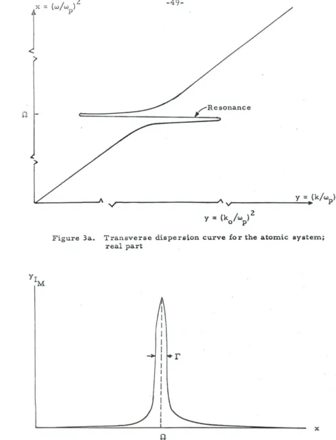
Equation II-65 is plotted in figure 3a. We see that. near the ori.gin.

- dx - l

-yRe

=

x with a slope

cry

=

1 -

in

•

1. At x .

0,

y It

0;

while

_

Ite

6

at x .

n

lit;

r.

YR

=

(1::1: - ) 0 - 10 (resonance): aa x - Q), YR - x.

e r e

The imaginary part of n-63 h

(U-66)

Equation II-66 18 plotted in figure 3b. We see that YIm 18 non-zero

only for x-

'1;

for x

=

0,

Ytm

=

¥

-105 - 107•

The alteration of the results for one excited state to the case of

many excited states is essentially that, instead of having one resonance

2/ 2 2/ 2 2/ 2

at x a ~ w

p ' there will be many resonances located at ~ wp' w2 wp'

• ••• The effect of the non-resonant states rn (see II-50) will in

general be very small compared to the resonant term. Specifically

at x

=

0 _n• YR _ea 0 _n(1

+

'

r), r «1, instead of YR .. x, whUe at _{n n e}

x ;: 0 •

r,

r can be ignored compared with 0 /

r.

The

imaii-n n n n n

nary part for many states gives a aeries of spikes at x · ,On', n •

1, 2, • •• •

For the atomic system, we are intereeted in values of K up to 2 3

the order of Ko. l/a_o• me - 10 Ryd. Thh h far beyond the

(53)

Yr

M

Resonance

c::::::=:==========:=::!::.~

_ _ _ _ _ _ _ _ _ y = (k/wp)2

~ Av~---~--··

y

=

(k

/w

)2

o P

Figure 3a. Transverse dispersion curve for the atomic system; real part

x

[image:53.614.71.562.40.683.2]

(54)

resonance region (see fieure 3a).

have

or

Now we go to the region of large K (Ka »1). From II-45 we

o

4 2 2

w 2 \1

+

z

rn w_lli ) • K2 • 0

(k

+

2rnw)(k - 2mw)

6 2 2 2 2

lt - 4m w (k • w ) • 0 _p (U·67)

Again. we will find solutions of 11-67 {or all K just as was done in the longitudinal case. For our atomic system we want the solution

for K» K _o

=

me2•

To aolve U-67 we first try to find aolutions for kZ

»

wZ•

p

11-67 becomes

or

2

k II .2mw

and

2 w

For 2mw to be much greater than wp implies that w» w (-1? )-p m

10-7 wp (for gases at S. T. P.). So {or w» 10.7 wp' the solutions

of k2

=

d: 2mw are

2 21/2 w :I d: m II: (m

+

K ) ;

(55)

and

K2

=

Z m + -_Zm

=K+m

for (K «m)

for (K» m)

W

z

III - m

+

(mZ

+

KZ)l/Z

KZ

::arm

=K-m

for (K« m)

for (K» m)

(U-68a)

(U-68b)

Again we see from

c.;,

that at KilO, W II 2m, i. e., a transverse

photon is able to make an electron position pair if its frequency b at

Z

least 2m. Now, W

z

=: K IZm

+ • ••

b a solution as long aa

w» W (w 1m) ::a 10-7 w which impliea that KZ

» "}.

So the

con-p con-p p p

dition. on W

z

are

for (w « K « m) • p

Now, the solution k2 =: 0 certainly does not aathfy kZ «

w~.

How-, Z Z

ever. to find the third solution try k ::a 6, where 6 - wp. We get,

3 Z 2. Z

from U-67, that 6 II 4m w (6 - w ), which baa the approximate

solu-p

tion 6 II w2. for w» w (w 1m) • 10-7

w.

Wo have kZ.

fl.?

or

p p p p p

Z KZ

+

2.

w III W

P (n-69)

For K

=

0, w

=

w (» 10-7 w) 80 U-69 is valid for all K. 'II-69

'p p

is recognized as the diaperDion formula for transverse wavea in a

, - Z 2

plasma for Pi::a O. (8). For K» w

(56)

the dispersion formula for free light. Now we fix up W

z

for K« wp.

For K

«w

•

p

Z Z

k I::S W • U-67 becomes

. w6 _ 4m Zw6(wZ_ wZ) :I 0

P

with solutions Z w

=

0

Z Z

w

=

w _p

and

Z

2.

W I: (lm)

w

=

wp is recognized as the limiting torm of n-69

tor

KZ

«

w! •

W

=

Zm is recognized as

"1

for K

=

O. Therefore. w:l 0 18 the

limiting form of W

z

for small K.The three solutiona are plotted in figure 4. Again we state that the portion of tho K axb that wo

are interested in is for K» meZ•

-We remark that the assumption Pi. 0 18 not a serious

limi-tation. We could. just as we did in the coulomb caso. rederive

everythi:lg with Pi "" O. From II-43' we find that the transverse

dielectric function (1'1. ) is ~r.

2

::.l+k

~

(57)

w

p

w p

r---~--~~---~~ k

k = mel

o

[image:57.613.67.555.56.615.2]

(58)

We note that for Pi rf. 0, the transverse and coulomb dielectric

func-tion are not equal. From II-70 we £ind, in the non-relativistic

ap-proximation, that the correction to the dhperaion lormula w2

=

K2

+w

2, P for small K, is

where

2 2 -2 [ K4

w=K+w 1+

Z::z

p 4m w

p

2

-2 2

w • _p w _p [ _{1 -}

b

5

<

_v2

> •

,,';1.

w]

2 K2

<v>-

~

2m

]

•

(n-71)

Except lor 11-71 we note that, in both the longitudinal and

transverse cases, the poles where wp (collective term) can be

nea-lected are identical (compare n-59 - II-61 with n-68 a, b). Thes.

poles correspond to single particle excitations by lonaitudinal and

transverse photons respectively: they should be equal, since a

particle which is initially at rest and picks up energy wand

momen-tum K from either a longitudinal or a transver.e photon must satisfy

(w :I- m)2 II KZ. mZ, which is just the determining relation for these

poles.

11-71 is the dispersion formula lor light propagating through the

medium, the w terms being the collective eUect of the medium on p

thia propagation, and