Generalised path following for well behaved nonlinear structures

Available online atwww.sciencedirect.com

ScienceDirect

Comput. Methods Appl. Mech. Engrg. 331 (2018) 394–426

www.elsevier.com/locate/cma

Generalised path-following for well-behaved nonlinear structures

R.M.J. Groh

, D. Avitabile

_{, A. Pirrera}

a_{Bristol Composites Institute (ACCIS), University of Bristol, Queen’s Building, University Walk, Bristol, BS8 1TR, UK} b_{School of Mathematical Sciences, University of Nottingham, University Park, Nottingham, NG7 2RD, UK}

Received 17 September 2017; received in revised form 27 November 2017; accepted 1 December 2017 Available online 6 December 2017

Abstract

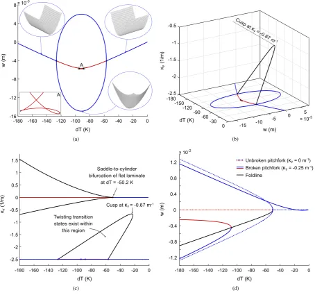
Recent years have seen a research revival in structural stability analysis. This renewed interest stems from a paradigm shift regarding the role of buckling instabilities in engineering design—from detrimental sources of catastrophic failure to novel opportunities for functionality. Novel nonlinear structures take the form of optimised thin-walled structures that operate safely in the post-buckling regime; shape-morphing structures that exploit multi-stability to snap and pop between different configurations; and meta-materials that derive novel material properties from a cascade of choreographed instabilities. Hence, elastic instabilities are no longer considered as structural failures but rather exploited for repeatablewell-behavedadaptations. In this article we focus on shape-morphing—a bio-inspired design strategy that intends to conform structures to different operating conditions. Computational tools that integrate easily with established methods used in industry, and that are capable of capturing the full phase diagram of compound instabilities and entangled post-buckling paths typical of these structures, are limited. Such a capability is crucial, however, as confidence in predictive tools can be key in enabling non-conventional designs. One potential candidate in this regard is generalised path-following, which combines the computational robustness of numerical continuation algorithms with the geometric versatility of the finite element method. In this paper we collate an array of successful computational tools introduced by other researchers, and introduce our own developments, to present a modelling framework fit for analysing and designing with well-behaved nonlinear structures in industry and academia. Particularly, we show that the full complexity of multi-snap events of morphing composite laminates is robustly captured by generalised path-following algorithms, and that the ability to determine loci of singular points with respect to a set of parameters is especially useful for tracing the boundaries of bistability in parameter space. Furthermore, we shed new insight into the mechanics of multi-stable laminates, showing that the multi-stability and snapping behaviour of these structures is much richer than previously assumed, featuring many unstable post-buckling branches and localised regions of stability.

c

⃝2017 The Author(s). Published by Elsevier B.V. This is an open access article under the CC BY license (http://creativecommons. org/licenses/by/4.0/).

Keywords:Generalised path-following; Nonlinear structures; Multi-functionality; Bifurcations; Morphing; Composites

∗

Corresponding author.

E-mail address:[email protected](R.M.J. Groh).

https://doi.org/10.1016/j.cma.2017.12.001

1. Introduction

To deliver the next generation of lightweight engineering structures, researchers and engineers are hoping to exploit, rather than avoid, elastic instabilities. Such designs could take the form of optimised thin-walled structures that operate safely in the post-buckling regime [1,2]; shape-morphing structures that snap between different configurations [3–11]; advanced meta-materials with innovative properties constructed from scale arrangements of mechanically multi-stable components [12–18]; and other diverse applications such as self-encapsulating structures [19] and fluidic soft actuators [20].

Indeed, there is an ongoing trend of shifting our intuitions about structural instabilities as sources of catastrophic failure to opportunities for functionality [21]. It is well known that efficient and lightweight structures are prone to structural instabilities and collapse [22,23]. In this case, the predominant design philosophy is to prevent buckling or at least make its effects benign. On the other hand, when reconfigurations in shape or large elastic displacements are required, buckling is often encouraged [24]. Reis [21] recently reviewed the burgeoning research effort focusing on exploiting instabilities to enable novel designs, and therefore provided a new perspective on buckling, namely from

buckliphobiatobuckliphilia.

In the aerospace industry, shape-morphing structures are viewed as a promising technology to enable more structurally efficient designs [3–11]. The premise behind this idea is simple—if structures can be designed to adapt their shape to more optimally conform to different loading conditions, then structural efficiency is improved as a result. In fact, this multi-functionality has a very strong empirical proponent: nature. Birds, for example, can adapt the camber and angle of attack of their wings to different flight scenarios. Even though some of the concepts found in nature are already being exploited in aircraft structures, such as slats and flaps, they often rely on rigid load-bearing components connected to heavy hydraulic or electric actuators. This is where multi-stable structures are particularly attractive. By applying a suitable force, a multi-stable structure can be snapped from one stable state to another, thereby considerably reconfiguring its shape. Because each stable state is self-equilibrated, it does not require external energy to hold its shape, and additionally, the sensing, actuation and control functions are embedded within the nonlinear mechanics of the structure (passive control) without adding additional mass via ancillary devices.

The uptake of these novel designs in industry is partly hampered by a lack of robust computational tools tailored to the design of structures whose characteristic feature is a form of spatial chaos [25],i.e. equilibrium manifolds featuring an entire series of bifurcations that give rise to many equilibrium branches and possible loading histories, especially in cases where dynamic snap-buckling is exploited for shape adaptation. Predicting these features reliably is pushing well-established finite element techniques to their limit, and is creating an acute requirement for new computational approaches for analysis and design [21,26]. In recent years the focus has been on analytical and computational techniques constrained to the analysis of very specific morphing problems with particular load cases and geometries [27–36]. A drawback of these tailored approaches is that simplifying assumptions are often made, which prevent applicability to a wider range of problems. Examples include restrictions on the geometric nonlinearity tovon K´arm´anstrains (small strains, small displacements and moderate rotations); posing the problem on a domain that is cumbersome to extend beyond simple geometries; and using nonlinear stability analyses without robust branch-switching.

Due to its geometric versatility and developmental maturity, the finite element method is the preferred technique for modelling complex structural problems. Commercial finite element packages may be used to analyse multi-stable structures [37–39], but most of the time, these analyses are ratherad hoc, because the full taxonomy of stable and unstable equilibria cannot be revealed robustly using the quasi-static implicit solvers implemented in these codes. Rather, the engineer needs to be aware of possible bifurcation pointsa priori, and then “coax” the algorithm to land on a specific post-buckling mode shape using initial imperfections. Such an approach is cumbersome and requires user intervention, such that it becomes difficult and inefficient to explore the entire design nonlinear space.

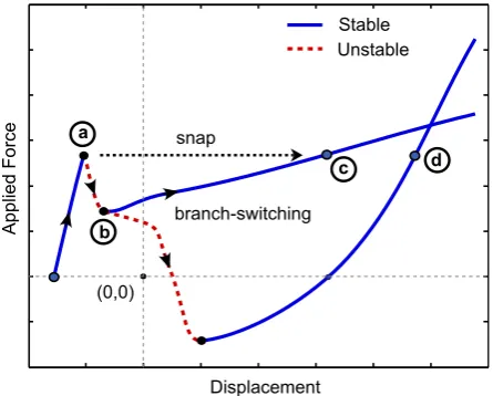
Fig. 1. Hypothetical example structure with typical snap-through equilibrium path illustrating the necessity for robust branch-switching. Without the ability to detect bifurcations and branch-switch, an engineer would not be aware of point (c) and presume that the structure snaps to point (d). Source:Adapted from [33].

of the existence of bifurcation point (b), stop the path-following algorithm before reaching it, run a linear eigenvalue analysis and then apply the lowest eigenmode as an imperfection. Such a procedure is cumbersome to implement and restricted to simple bifurcation points (for compound bifurcations there is little control over which branch the solver will converge to). Finally, when conducting design sensitivity studies, the full equilibrium paths of different design iterations need to be traced, when the designer is, in fact, only interested in how certain points,e.g.critical points (a) and (b), vary with a particular design parameter.

Thus, the ideal computational framework for structures exploiting instabilities includes, but is not limited to, the following characteristics:

1. Applicable to arbitrary (thin-walled) geometries.

2. Applicable to large displacements and rotations,e.g.total Lagrangian framework, such that a large variety of structural instabilities are accounted for.

3. Able to detect singular points and branch-switch onto secondary paths without recourse to initial imperfections. 4. Allows for rapid parametric studies of critical points with respect to any geometric, constitutive or secondary

loading parameter.

5. Is readily integrated with accepted computational methods used in industry, predominantly, the finite element method.

One possible framework that addresses all of these points is the so-calledgeneralised path-following method, which provides the means to systematically explore the design space of multi-stable structures with respect to a given parameter set. The termgeneralised pathwas probably coined by Eriksson [40], where it referred to a multi-parametric setting of static equilibrium problems that extends the notion of applied load as the only active control parameter, and it is this definition that we refer to herein. Historically, generalised path-following has been used extensively in the fields of applied mathematics and physics [41–46], where the term numerical continuationis a more common designation. In engineering applications, however, path-following in load–displacement space, typically a variant of the Riks method [47], is a familiar term, such that generalised path-following is an intuitive extension to a multi-parametric setting.

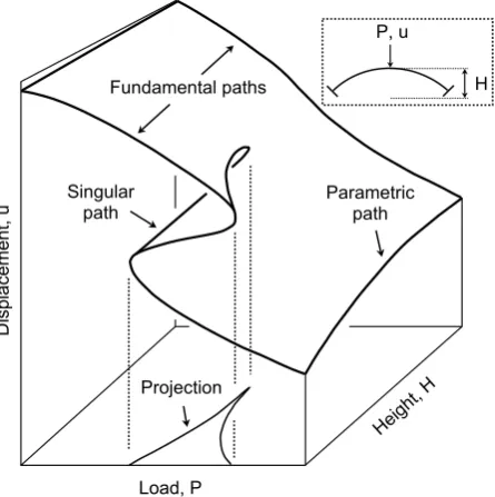
Fig. 2.An equilibrium surface for the snap-through behaviour of an elastic arch. In a generalised path-following algorithm different paths on this equilibrium surface can be traced by defining particular auxiliary equations. For example, the figure shows a fundamental path in load–displacement space (height held constant), a parametric path in height–displacement space (load held constant), and a singular path in load–height–displacement space connecting the limit points for different arch heights.

Source:Adapted from [50].

concepts allowed pinpointing of singular points (bifurcation and limit points); branch-switching at bifurcation points; path-following with respect to any parameter,e.g.load, thickness, Young’s modulus, dimensions,etc.; and tracing loci of bifurcation and/or limit points in multi-parametric space (see Fig. 2). In this sense, generalised path-following extends concepts from computational bifurcation theory [58–60], such as path-tracing, pinpointing of singular points and branch-switching, from a single- to a multi-parametric setting. Starting from the mid-1990’s, Eriksson and co-workers [40,61–65] established themselves as the main developers of generalised path-following, presenting numerous examples in structural engineering where the approach proved to be of great benefit, while also providing details on how the technique could be incorporated into commercial nonlinear finite element codes. Similarly, within the broader applied mathematics community, the Library of Continuation Algorithms (LOCA) was developed by Sandia National Laboratories to deal with large degree-of-freedom problems, typically arising from the discretisation of partial differential equations but not necessarily restricted to finite elements, to be run on parallel computing platforms [44]. In engineering, numerical continuation has also been successfully applied to study nonlinear phenomena in the fields of aerodynamics [66–68], aeroelasticity [69–71] and the analysis of cylindrical shells [33,72–74].

snap-through phenomenon, showing that the snapping behaviour is much richer than previously assumed, featuring many entangled secondary post-buckling paths with localised regions of stability, and using the bifurcation-tracking capability to delineate regions of bistability in parameter space.

2. Theory

A generalised path-following algorithm combines the mathematical domains of finite element analysis and numerical continuation. The mathematical methods used in numerical continuation are well established [41–43,45,56], but are not classically used for structural mechanics applications, where specialised arc-length techniques are predominant [47,76]. The present formulation considers a discretised model of a slowly evolving, conservative and elastic structure, where the internal forces and tangential stiffness are uniquely defined from the current displacements by means of the first and second variations of an energy potential. Thus, non-conservative loading and history-dependent problems such as plasticity are not included in the current formulation.

In Section 2.1 we proceed with the general framework and then discuss implementation-specific details in Sections 2.2–2.3. The interested reader is also especially encouraged to consult the excellent expositions by Eriksson [40,61,62] which form the basis of the theory. Finally, an accurate analysis using these numerical methods depends on suitable choices of nonlinear beam and shell elements that have sufficient fidelity to capture the full complexity of nonlinear instability phenomena (see [77,78]).

2.1. The general setting

In classical structural mechanics applications, equilibrium is expressed as a balance between internal and external forces, where, in a displacement-based finite element setting, this balance is written in terms ofndiscrete displacement degrees-of-freedom,u, and a scalar loading parameter,λ,

F(u, λ)=f(u)−p(λ)=0. (1)

The vectorsp(λ) andf(u) are the external (non-follower) load and internal force, respectively. In the case of linear and proportional loading we havep(λ)≡λp_,λ1 _{=λpˆ, wherepˆis a constant reference loading vector (dead loading). This} system ofnequations in (n+1) unknowns –ndisplacement degrees-of-freedom and one loading parameter – is then solved for a solution point,x=(u, λ), by defining an additional scalar arc-length constraint,N(x)=n⊤

uu+nλλ−σ,

such that

FN(x)≡ (

F(x)

N(x)

)

=0, (2)

wherenu andnλtake different forms depending on the nature of the arc-length constraint. By linearising about the

current equilibrium state,x, and applying Newton’s method for the iterative correction,δx,

FN(x+δx)=FN(x)+FN_,x(x)δx+O(δx2)≡0

⇒δx= −(

F_,N_x(x))−1

FN(x), (3)

we can find a set of solution points that describes a continuous equilibrium curve. Note that the partial derivative of the residual with respect to the displacement vector,F_,u=f,u(u), is equal to the tangential stiffness matrixKT(u).

For generalised path-following, Eq.(1)is adapted to incorporate any number of additional parameters,

F(u,Λ)=f(u,Λ1)−p(Λ2)=0, (4)

whereΛ=[Λ⊤

1,Λ

⊤

2]

⊤_{=[λ1, . . . , λ}

p]⊤is a vector containingpcontrol variables.Λ1corresponds to parameters that

influence the internal forces (e.g.material properties, geometric dimensions, temperature and moisture fields) andΛ2

relates to externally applied mechanical loads (e.g.forces, moments, tractions).

Thennumber of equilibrium equations in Eq.(4), correspond directly to thennumber of displacement degrees-of-freedom in the system. Because the structural response is parametrised by padditional parameters, a p-dimensional solution manifold inR(n+p) _{exists—the so-calledequilibrium hypersurface [48]. By defining additional auxiliary}

equations,g, specific solution subsets on thisp-dimensional solution manifold are defined. Hence, we wish to evaluate solutions to the augmented system

G(u,Λ)≡ (

F(u,Λ)

g(u,Λ)

)

=0. (5)

Whenr auxiliary equations are defined, the solution to Eq.(5)is (p−r)-dimensional. Hence,r = p−1 auxiliary equations are required to define a one-dimensional curve, or so-calledsubset curve[62], inR(n+p).

Posing the problem in this manner allows the structural response to be viewed not only as a function of a varying load but also as a function of other parameters that define the structure. By treating these additional parameters as “forcing” variables in an arc-length solver, the effect of these parameters on the structural response can be obtained. Hence, the computationally expensive approach of studying variations in geometry and material properties, by evaluating full load–displacement equilibrium curves for each additional model, is avoided. Instead, different load–displacement or parameter–displacement paths are described as cutsets of a higher-dimensional solution surface (seeFig. 2).

This treatment naturally leads to the notion of tracing loci of singular points in parameter space, such as the maxima and minima shown inFig. 2. As the designer of multi-stable structures is predominantly interested in critical instability points,e.g.limit points that initiate snap-through or symmetry-breaking bifurcations, these singular curves are invaluable for rapidly exploring the design space. To constrain the system ofn equilibrium equations to a locus of singular points, we simultaneously enforce the fulfilment of a criticality condition, for exampleKTφ =0,i.e.at

least one eigenvectorφof the tangential stiffness matrixKTspans the nullspace. In the most general form, not limited

to but including the previous criticality condition, a vector ofq auxiliary variables,v, may be added to the auxiliary equationsg,

G(u,Λ,v)≡ (

F(u,Λ)

g(u,Λ,v)

)

=0. (6)

Hence, Eq.(6)describesn equilibrium equations andr auxiliary equations in (n +p+q) unknowns leading to a (p+q−r)-dimensional solution. To determine a one-dimensional subset curve of singular points, we thus require

r =p+q−1 auxiliary equations to constrain the system. Following the example from above, when then-dimensional null vector at the critical state is introduced as the auxiliary variable,v, a singular subset curve in two parameters,

p=2, is appropriately constrained by the associatedr=n+1 auxiliary equationsKTv=0and∥v∥2=1, where the

scalar equation restricts the magnitude of the eigenvector.

When evaluating one-dimensional subset curves (r = p+q−1), one additional constraining equation is needed to uniquely solve the system of equations for a solution point y = (u,Λ,v) on the curve described by G(y). Hence,

GN_(y)≡

⎛

⎝

F(u,Λ)

g(u,Λ,v)

N(u,Λ)

⎞

⎠=0, (7)

whereNis a scalar equation that plays the role of a multi-dimensional arc-length constraint along a specific direction of the subset curve. Note that the system of equations for classical load–displacement equilibrium paths can be recovered by setting p=1 andq =r =0. A solution to Eq.(7)is determined by a consistent linearisation coupled with Newton’s method,

y_kj+1=y_kj−(G_,N_y(y_kj)) −1

GN(y_kj)≡y_kj+δy_kj, (8)

where the superscript denotes the jth equilibrium iteration and the subscript thekth load increment. The iterative correction cycle is typically started by a predictive forward Euler step. For most problems, the inversion of the iteration matrix,

G_,N_y= ⎡

⎣

F_,u F,Λ 0n×q

g_,u g,Λ g,v

N_,⊤_u N_,⊤_Λ 01×q

⎤

⎦, (9)

Within this framework, the meaning of the termgeneralised path-followingbecomes clear. It refers to the fact that any arbitrary curve can be traced on the equilibrium surface, as long as a pertinent auxiliary equation is defined that constrains the equilibrium equation to the locus of points required. These auxiliary equations can define, but are not necessarily limited to, the following interesting paths:

• Classic equilibrium paths in load–displacement space (a loading parameter is varied).

• Parametric paths in parameter–displacement space (a geometric, constitutive or secondary loading parameter is varied).

• Pinpointing singular points (bifurcation and limit points) on either of the two paths mentioned above.

• Bifurcated branches emanating from a bifurcation point.

• Singular paths that describe a locus of bifurcation and/or limit points in load–parameter–displacement space.

• Branch-connecting paths that connect points on distinct equilibrium curves.

Furthermore, auxiliary equations have also been devised to define optimality criteria [82] and to directly evaluate the imperfection mode shape that leads to the greatest knock-down in the buckling load of compressed cylindrical shells [83].

2.2. Path-following in one parameter

The parametersΛ = (λ1, . . . , λp) can be any set of p parameters that affect the equilibrium of the structure.

In a structural engineering context, it is pertinent to treat parameterλ1as the fundamental loading parameter, here mechanical or thermal in nature, such that path-following inλ1traces the fundamental load–displacement equilibrium path of an idealised baseline model. Parameters Λs = (λ2, . . . , λp) are then added as secondary parameters that

perturb this idealised baseline problem,e.g.variations in geometry, changes to constitutive properties or the addition of secondary loadings. Any saved equilibrium solution on the fundamental path then serves as a starting point for path-following in a secondary parameter,λs∈ Λs, thereby tracing a parametric path of perturbed equilibrium points

withλ1constant.

Due to the practical limitation of visualising results in three dimensions, the present implementation is posed in terms of the displacement degrees-of-freedom,u, the fundamental loading parameter,λ1, and a secondary parameter,

λs∈Λs, such that a pertinent norm of the displacement vector,e.g. uifori =1. . .n, can be plotted against (λ1, λs).

The results for different combinations of (λ1, λs) are therefore plotted in succession. For clarity, fundamental and parametric paths are first discussed individually in Sections2.2.1and2.2.2, respectively, with all equations expressed in terms of (λ1, λs) only, and all other parameters removed from consideration (kept constant at baseline values). Section2.2.3then generalises the notation to any non-critical subset path with only one varying parameter. The topic of pinpointing singular points on these paths is then discussed in Section2.2.4.

2.2.1. Fundamental paths

The system of equations for classical load–displacement equilibrium paths can be recovered by settingp =1 and

q=r=0 such thatλ1becomes the fundamental loading parameter. In the case of linear and proportional mechanical loading,

F(u, λ1)=f(u)−λ1pˆ1=0. (10)

In the case of thermal loading,λ1affects the internal force vector andpˆ1=0, such that

F(u, λ1)=f(u, λ1)=0. (11)

Introducing the scalar arc-length constraintN(u, λ1), as defined in Eq.(2), and applying Newton’s method

[

F_,u F_,λ1

N_,⊤_u N_,λ1

] { δu

δλ1 }

= − {

F(u, λ1)

N(u, λ1)

}

, (12)

whereδuandδλ1are iterative corrections of the nodal displacements and loading parameter, respectively.F_,u≡KTis

the tangential stiffness matrix andF_,λ1 = − ˆp1is the reference loading vector for linear and proportional mechanical

the reference force vector is derived frompˆ1 = −KCuc,i.e.the constrained portion of the tangential stiffness matrix

multiplying the non-zero prescribed displacements. As the tangential stiffness matrix is generally a function of current displacements, the reference force vectorpˆ1 derived from prescribed displacements needs to be updated for every

iteration of the solution scheme.

In the case of thermal loading, the effective strain method described by Parente Jr et al. [84] is applied. The effective strain is given by the difference between the classic geometric strain, here the Green–Lagrange strain,ϵGL, and the

free thermal strain,ϵth. The thermal strain,

ϵth=α∆T, (13)

represents the strain induced when thermal expansion of the material is not constrained, with α representing the thermal expansion coefficient vector and∆T the change in temperature. For linear elastic materials, the stress–strain– temperature relation can be written as

σ(u, λ1)=CT(ϵGL(u)−ϵth(λ1))=CT (

ϵGL−αλ1∆Tˆ )

, (14)

whereσ is the energetically conjugate second Piola–Kirchhoff stress tensor and∆_Tˆ _{is a temperature change from a}

given strain-free reference temperature. In general, the tangent constitutive tensor,CT, is temperature dependent.

In the context of the principle of virtual displacements the internal force vector, used in Eqs.(10)–(11), is given by

δu⊤f = ∫

V δϵ⊤_σ

dV = ∫

V

δ(ϵGL−αλ1∆Tˆ )⊤

σdV = ∫

V δϵ⊤

GLσdV. (15)

By assuming a general relation between the virtual geometric strain and the virtual displacements,δϵGL(u)=B(u)δu,

and substituting Eq.(14)forσ, the internal force vector for a thermal loading problem is

f(u, λ1)= ∫

V

B⊤_σ dV =

∫

V

B⊤_C

T (

ϵGL−αλ1∆Tˆ )

dV. (16)

The precise definition of the kinematic matrix,B, depends on the chosen finite element implementation and shape function interpolation, and is therefore not discussed in detail herein. The tangential stiffness matrix,KT, and the

thermal load vector,pˆth, are derived from the variation of Eq.(11):

δF(u, λ1)=F_,uδu+F,λ1δλ1=f,uδu+f,λ1δλ1=KTδu+ ˆpthδλ1. (17)

In particular, the variation of Eq.(16)with respect tougives:

f_,uδu≡KTδu= ∫

V

B⊤CTδϵGLdV+ ∫

V δB⊤CT

(

ϵGL−αλ1∆Tˆ )

dV

= ∫

V

B⊤CTBdV δu+ ∫

V δB⊤CT

(

ϵGL−αλ1∆Tˆ )

dV =[Ke+Kg ]_δ

u. (18)

Eq.(18)shows that the elastic stiffness matrix,Ke, is unchanged from the classical linear stiffness matrix and not

affected by temperature changes. Even though the geometric stiffness matrix,Kg, always depends on the particular

element formulation chosen, Eq.(18)shows thatKgis a function of temperature changes via the current stresses,σ.

This means that the tangential stiffness matrix is only affected by temperature changes through the geometric stiffness component.

Similarly, the thermal load vector is given by the variation of Eq.(16)with respect toλ1,

f_,λ1δλ1= ˆpthδλ1= − ∫

V

B⊤CTα∆TˆdV δλ1, (19)

where we have assumed that the tangential constitutive tensorCTdoes not vary with temperature. If the constitutive

tensor does vary with temperature then the termCT_,λ1 needs to be computed. In this case it is most convenient to

evaluate an approximation topˆthusing a forward difference scheme,

ˆ

pth=f,λ₁ ≈

f(u, λ1+ε|λ1|)−f(u, λ1)

ε|λ1| , (20)

whereεis a small perturbation parameter typically in the range of 10−5_{to 10}−8_{. The default choice ofεin Eq.(20),}

ofεwithin the range [10−5_,10−8]

is robust, meaning that the convergence of Newton’s method is not sensitive to changes inε. Even though the accuracy of this numerical approach depends on the choice ofε, and is computationally less efficient than a direct approach, it has the advantage of being valid for all element types, and is therefore readily implemented in existing codes. In either case, it is important to remember that the thermal load vector needs to be iteratively updated during the entire thermal loading process, becauseBis a function of the current displacementsu.

Finally, the form of the arc-length constraint depends on the particular method chosen, although in our experience, the planar constraint by Riks [47] and the cylindrical constraint by Crisfield [76] work most robustly. The details of different arc-length constraints are covered extensively in textbooks and many publications (seee.g.[84–87]), and are therefore not elucidated in further detail here. Some implementation-specific comments are nevertheless warranted.

• Given the quadratic nature of Crisfield’s cylindrical arc-length constraint [76], two roots for the iterative correctionδλ₁j_k (of the jth equilibrium iteration and the kth load increment) arise, and if both of these are imaginary, or real and negative, it is easiest to repeat the current load increment with a reduced incremental arc-length.

• When both roots are real and positive, the root that is closest to the root of an analogue linear system (simply ignoring the quadratic term) is chosen. When one of the real roots is positive and the other negative, the positive real root is chosen.

• The sign of δλ1

1k,i.e. the load predictor in the first iteration of each increment k, is readily determined by

taking the dot product between the total incremental displacement of the previous step,∆uk−1, andδu1k,i.e.the

displacement predictor in the first iteration of the current step calculated from the unit load vector 1· ˆp1or 1· ˆpt h.

Ifδλ1

1kis defined to take the sign of this dot product, then limit points are easily traversed.

Noting these caveats, Crisfield’s cylindrical arc-length constraint [76] performs very robustly for both fundamental and parametric paths, including the traversal of turning and snap-back points, and is therefore explicitly used for the problems studied in Section3and in Section4.

2.2.2. Parametric paths

Any equilibrium solution on a fundamental path can be used as a starting point for path-following in one of the secondary parameters,λs ∈ Λs. In this manner, the sensitivity of the baseline design to variations inλsis assessed.

For example, if the basic topology of the problem is to be kept constant we may parametrise a specific geometric dimension asL(λs) = L0(1+cλs), which can be used to analyse the effects of thickness, length or height on the

structural behaviour. Equally, we may add a mode shape, β, to the nodal coordinates of the basic geometry, x0,

such thatx0(λs)=x0+cλsβ, which can be useful for imperfection sensitivity studies or parametrically varying the

topology of the problem. Similarly, we may study the effects of constitutive properties, such as Young’s modulus

E(λs) = E0(1+cλs). Finally, a secondary loading ps = cλspˆs may be added to study the combined load case

p=λ1pˆ1+cλspˆs, which may be interpreted as studying the effect of either loading under the perturbing influence of

the other. In all cases, it may be necessary to scale the secondary parameter,λs, by a factor,c, such that the order of magnitude of the two parameters is similar,i.e.O(λ1)≈O(λs).

The methods introduced in the previous section can readily be adapted to parametric paths. In the current notation there are three different combinations ofλ1 andλs, with λ1 held constant in each case. For combined mechanical loading

F(u, λ1, λs)=f(u)−λ1pˆ1−λspˆs=0. (21)

Alternatively, for fundamental mechanical loading with secondary thermal loading, geometrical changes or constitu-tive variations

F(u, λ1, λs)=f(u, λs)−λ1pˆ1=0. (22)

Finally, for fundamental thermal loading with secondary thermal loading, geometrical changes or constitutive variations

F(u, λ1, λs)=f(u, λ1, λs)=0. (23)

Introducing the scalar arc-length constraintN(u, λs) and applying Newton’s method

[

F_,u F_,λs

N_,⊤_u N_,λs

] {_δ

u

δλs }

= − {

F(u, λ1, λs)

N(u, λs)

}

whereδu andδλs are iterative corrections of the nodal displacements and secondary parameter, respectively. For secondary linear and proportional mechanical loadingF_,λs = − ˆps. Otherwise, F,λs is calculated from a forward

difference scheme,

F_,λs =f_,λs ≈ f(u, λ1, λs+ε|λs|)−f(u, λ1, λs)

ε|λs| , (25)

whereε is a small perturbation parameter typically in the range of 10−5 to 10−8. Finally, the caveats regarding Crisfield’s cylindrical arc-length constraints raised in the previous section are equally valid here.

2.2.3. Single-parameter non-critical subset paths

To illustrate the general concepts of continuing in load–displacement and parameter–displacement space, the equations in the previous two sections are purposely restricted to fundamental parameterλ1and secondary parameter

λs. These concepts are now combined to generalise the notation to any path with only one varying parameter (fundamental or parametric), also known as a non-critical subset paths in one parameter [40]. Hence,

F(u, λ1,Λis,Λe_s)=f(u,Λi_s)−λ1pˆ1− ˆPsΛes=0, (26)

for fundamental mechanical loading, and

F(u, λ1,Λi_s,Λe_s)=f(u, λ1,Λi_s)− ˆPsΛes=0, (27)

for fundamental thermal loading.Pˆs is a matrix of column-wise secondary load vectors, andΛisandΛes parametrise

internal and external force vectors, respectively. Each parameter takes the value that describes a baseline design and then one target parameter,λt∈(λ1,Λi_s,Λe

s), is varied to trace a particular equilibrium path, while all other parameters

Λc⊂(λ1,Λis,Λes), λt̸∈Λcare held constant. Hence,

GN(u, λt,Λc)≡ ⎛

⎝

F(u, λt,Λc)

Λc−Σ

N(u, λt)

⎞

⎠=0, (28)

whereΣis the set of prescribed constant parameters andN(u, λt)=n⊤

uu+nλtλt−σis a general arc-length constraint.

Linearisation yields

⎡

⎣

F_,u F_,λt F,Λc 0(p−1)×n 0(p−1)×1 1(p−1)×(p−1)

n⊤

u nλt 01×(p−1) ⎤

⎦ ⎧

⎨

⎩ δu

δλt δΛc

⎫

⎬

⎭ = −

⎧

⎨

⎩

F(u, λt,Λc)

Λc−Σ

N(u, λt)

⎫

⎬

⎭

(29)

where1 is the identity matrix. The 2nd row and 3rd column of the iteration matrix can generally be omitted as

δΛc=0by definition. Similar to classical arc-length methods [76], the iteration matrix in Eq.(29)is never inverted

in its entirety but split into the blocks shown, and then solved via a partitioning procedure and back-substitution such that onlyF_,u≡KTneeds to be inverted [76] (seeAppendix).

2.2.4. Pinpointing singular points

Pinpointing singular points is useful for evaluating the exact value of snap-through loads (to within a certain tolerance) and for ascertaining the existence of bifurcations onto other branches. Furthermore, unfolding of these singular points with respect to other parameters can provide invaluable insights into imperfection and design parameter sensitivity.

Remark(Singular Points). Using a Taylor series expansion, a small change in the energy potential,Π(u,Λ), of a conservative elastic system is

δΠ = ∂Π ∂uδu+

1 2δu

⊤∂

2_Π

∂u2δu+O(δu

3_)=F⊤_δ

u+1

2δu ⊤

KTδu+O(δu3), (30)

and unvaried parametersΛc, may thus be determined byδu⊤_{KTδu =0 for all arbitraryδu. This coincides with the} condition that

detKT(u∗, λ∗t,Λ

∗

c)=0⇒KT(u∗, λ∗t,Λ

∗

c)φ=µφ=0. (31)

Here, µ = 0 is the eigenvalue that corresponds to the critical eigenvector φ at the singular point (u∗_{, λ}∗

t,Λ

∗

c).

Parametrising the equilibrium equations further in terms of an arc-length parameter,s, and differentiating with respect to this curve parameter gives

˙

F(u(s), λt(s),Λc(s))=F_,uu˙+F_,λtλt˙ +F,ΛcΛ˙c=KTu˙+F,λtλt˙ =0, (32)

where a superimposed dot denotes differentiation with respect tos. Given the symmetry ofKT and the singularity

condition Eq.(31), pre-multiplication of Eq.(32)byφ⊤at a singular point yields

[

φ⊤

F_,λt(u∗, λ∗_t,Λ∗_c)]λt˙ =0. (33)

Hence, on an equilibrium path in one parameter (fundamental or parametric) there can only be two types of singular points—a limit point,i.e.a local extremum withλt˙ =0 andφ⊤F_,λt ̸= 0, or a bifurcation point,i.e.an intersection between two or more distinct equilibrium curves withφ⊤F_,λt =0. For numerical consistency, the latter condition is typically implemented as φ

⊤_F

,λt

∥φ∥₂·∥F_,λt∥₂ < εwith 10

−5 _{< ε < 10}−2_{. The choice ofεis not calculated automatically}

but from experience based on a “good guess” of 10−3_{. From the equilibrium curve, it is typically straightforward to}

ascertain if a critical point should be a limit point or not, and in the rare cases where the choice ofε= 10−3_{is not}

sufficient, the tolerance can be reducedad hoc.

The second derivativeF¨ =0can be used to determine the two tangent vectors at a simple bifurcation point – one tangent to the primary path and the other tangent to the secondary bifurcated path – and also to classify the type of bifurcation—pitchfork, transcritical, isola formation point or cusp point. The disadvantage is that the derivative

KT,u needs to be computed approximately via finite differences, with an associated penalty in computational cost.

For computational efficiency, these calculations are not performed herein and the interested reader is directed to Refs. [84,88].

To pinpoint singular points, an augmented system of the form described in general by Eq.(7) is formulated. A number of different auxiliary equations are defined in the literature for this purpose,e.g.g=µ=0,g=det(KT)=0,

g = KTφ = 0,etc., as outlined in the comparative review by Melhem & Rheinboldt [89]. The advantage of this

method is that the singularity condition forces Newton’s method to converge to the singular point directly in a single increment. Although bisection techniques have also been developed [59,88], they require the calculation of multiple intermediate equilibrium points to hone in on the singularity and are thus computationally more expensive.

In the present finite element setting, the nullvector approach described by Wriggers et al. [80,81] – generally first presented by Seydel [90] and Moore & Spence [91] – and the minimally augmented method introduced by Griewank & Reddien [92], and further developed by Eriksson [61] and Battini et al. [93], are used. The minimally augmented technique is chosen by default in the developed computer program, and the nullvector method used as an alternative option when the former has trouble converging.

The nullvector method is based on the fact that the tangential stiffness matrix,F_,u ≡ KT, has at least one zero

eigenvalue,µ=φ⊤KTφ, at a singular point. Therefore, the associated eigenvector,φ, is in the nullspace ofKT. Thus,

the augmented system is written as

G(u, λt,Λc,φ)≡ ⎛

⎝

F(u, λt,Λc)

KT(u, λt,Λc)φ ∥φ∥₂−1

⎞

⎠=0, (34)

where the norm of the nullvector is required to eliminate the trivial solutionφ=0. Eq.(34)features (2n+1) equations in (2n+p) variables, and the (p−1) extra equations required to solve the system are implicit in the definition that the added control parameters inΛcare held constant,i.e.Λcj=Σjfor j =2. . .p(see Eq.(29)). The resulting system of

equations can therefore be solved in the usual manner via Newton’s method for a singular point, (u∗_{, λ}∗

t,Λ

∗

c), as well

the linearisation of Eq.(34),

⎡

⎢ ⎢ ⎢ ⎣

KT F,λt 0 (KTφ)_,u (KTφ)_,λt KT

01×n 0

φ⊤

∥φ∥₂ ⎤

⎥ ⎥ ⎥ ⎦

⎧

⎨

⎩ δu

δλt δφ

⎫

⎬

⎭ = −

⎧

⎪ ⎨

⎪ ⎩

F(u, λt,Λc)

KT(u, λt,Λc)φ ∥φ∥₂−1

⎫

⎪ ⎬

⎪ ⎭

. (35)

Following the reasoning by Wriggers & Simo [81], approximate directional derivatives of the tangential stiffness matrix can be computed as follows,

(KTφ)_,u≈

KT(u+ε∥u∥2φ, λt,Λc)−KT(u, λt,Λc)

ε∥u∥₂ , (36)

(KTφ)_,λt ≈

KT(u, λt+ε|λt|,Λc)−KT(u, λt,Λc)

ε|λt| φ, (37)

withεin the range of 10−5 to 10−8. As noted before, a seemingly robust default choice isε = 10−8, although it is possible that at some bifurcation points Eqs.(36)–(37)may become sensitive to changes in ε, and in these cases a central difference scheme may be more appropriate for good convergence of Newton’s method.

Whenλtis a primary or secondary displacement-independent mechanical loading parameter,(KTφ)_,λt vanishes

andF_,λt equals− ˆp1or− ˆps. Otherwise,F_,λt is approximated by

F_,λt =f_,λt ≈ f(u, λt+ε|λt|,Λc)−f(u, λt,Λc)

ε|λt| . (38)

When solving the system of equations in Eq.(35), the iteration matrix is not inverted in its entirety, but split into individual blocks (as shown), and solved by a partitioning procedure in such a manner that only the symmetric tangential stiffness matrix needs to be factorised (seeAppendixand Wriggers & Simo [81] for the general algorithm). This means that the computational cost of pinpointing is similar to that of a standard arc-length continuation step, especially for large degree-of-freedom systems, where the factorisation ofKTdominates.

The present computer implementation proceeds as follows. While continuing along a fundamental or parametric equilibrium path, the 20 smallest magnitude eigenvalues of the tangential stiffness matrix are monitored. This can be done efficiently for large yet sparse tangential stiffness matrices by using the FORTRAN Arnoldi package ARPACK [94], embedded in many popular numerical computing environments such as MATLABand SCIPY. When the number of negative eigenvalues between two consecutive converged equilibrium solutions changes, a singular point must exist between these two converged equilibria and the pinpointing procedure is started. The number of singular points present depends on the change in the number of negative eigenvalues,N∗_{. The set of eigenvectors,Φ,} associated with the smallestN∗ _{eigenvalues at the last converged equilibrium state, (u}l_{, λ}l_t,Λl

c), are then extracted,

and eachφj ∈ Φfor j =1. . .N∗_{consecutively seeded alongside (u}l_{, λ}l_t,Λl

c) as the starting point for the iterative

pinpointing procedure. In our experience, this eigenmode seeding procedure works reliably for one singular point, as well as multiple distinct or coincident (compound) singular points. If the solver does not converge, then an additional equilibrium point between the two previously determined equilibria is determined and the process is repeated. This is typically the case when the nonlinearity between the last converged equilibrium state,i.e.the starting point, and the singular point is too high.

In the minimally augmented method [92], the vector equationKTφ=0is replaced by the scalar equation

µ=φ⊤KTφ=0, (39)

whereµis an eigenvalue of the symmetric tangent stiffness matrix,KT, andφthe associated eigenvector. By definition, µmust vanish at a singular point such that φbecomes a nullvector of KT. The scalar equation(39)is derived by

pre-multiplying the eigenvalue problem,KTφ=µφ, withφ⊤and enforcing the normalisation constraintφ⊤φ=1.

Rather than computing the singular point (u∗, λ∗_t,Λ∗

c) and the associated nullvectorφsimultaneously (as is done

in the nullvector method),µandφare determined separately. Thus, as a first step the eigenvalue problem is written as an iterative problem [93]

KTφk+1=µk+1φk, (40a)

φ⊤

where the latter equation (40b) now constrains the updated eigenvector to be parallel to the previous one with

∥φ_k+1∥₂ = ∥φ_k∥₂ =1. Note, by pre-multiplying Eq.(40a)withφ⊤_k+1and heeding Eq.(40b), we recover the scalar conditionµk+1=φ

⊤

k+1KTφk+1. Eqs.(40a)–(40b)are rearranged into matrix form as follows: [

−KT φk φ⊤

k 0

] {_φ

k+1 µk+1 }

= {

0

1

}

. (41)

Eq.(41)is solved efficiently using a partitioning procedure by first computing an immediate vectorϕ =K_T−1φ_k, and then back-substituting to findµk+1 =1/(φ⊤kϕ) and subsequentlyφk+1 =µk+1ϕ. With an arbitrary random starting

vector,φ₀, the iteration scheme converges to the smallest magnitude eigenvalue and associated eigenvector typically within 2–3 iterations. When starting the algorithm with an informed, non-arbitrary approximation of a particular eigenvector, the solver refines the eigenvector and returns the associated eigenvalue often within a single iteration.

As a second step, the equilibrium equations are augmented with the scalar singularity condition of Eq.(39),

G(u, λt,Λc)≡ (

F(u, λt,Λc) µ(u, λt,Λc) )

=0. (42)

Eq.(42)features (n+1) equations in (n+p) variables, and the (p−1) extra equations required to solve the system are again implicit in that parametersΛctake prescribed values. A singular point (u∗, λ∗t,Λ

∗

c) is calculated via Newton’s

method using the iteration matrix

[

KT F,λt µ⊤

,u µ,λt ]

{_δ

u

δλt }

= − {

F(u, λt,Λc) µ(u, λt,Λc) }

. (43)

The differentials of the scalar singularity condition are computed via finite difference approximations,

µ,u≈φ⊤

KT(u+ε∥u∥2φ, λt,Λc)−KT(u, λt,Λc)

ε∥u∥₂ , (44)

µ,λt ≈φ

⊤KT(u, λt+ε|λt|,Λc)−KT(u, λt,Λc)

ε|λt| φ, (45)

withεin the range of 10−5 _{to 10}−8_{. As mentioned previously, if the choice ofε = 10}−8 _{does not provide good}

convergence for some bifurcation points, then a central difference scheme may be used for better results. Whenλtis a primary or secondary displacement-independent mechanical loading parameter,µ_,λt vanishes andF_,λt equals− ˆp1or − ˆps. Otherwise,F,λtis approximated by Eq.(38). Eq.(43)is solved in a typical manner using a partitioning procedure

by first determiningδu1 = −KT−1Fandδu2 = −KT−1F,λt, and then back-substituting to findδλt = −

µ+µ⊤_,uδu1 µ,λt+µ

⊤

,uδu2 and

subsequentlyδu=δu1+δλtδu2.

The minimally augmented method therefore requires two iteration steps to be performed in succession—the main iteration loop performed on Eq. (43) to converge the solution (u, λt) closer to a singular point, followed by an embedded iteration loop via Eq. (41) to update the eigenvalue and eigenvector for each iteration of (u, λt). The pinpointing algorithm is again initiated by consecutively seeding a particular eigenvectorφ0=φj ∈Φ, j =1. . .N

∗

in the set of eigenvectors, Φ, associated with the smallest N∗ _{eigenvalues of K}

T that changed sign between the

last two converged equilibrium solutions (see description for the nullvector method on page 13). Hence, the N∗

eigenvalues and eigenvectors at the last converged equilibrium state, obtained in a computationally efficient manner from ARPACK [94], serve as starting points for pinpointing a set ofN∗_{singular points.}

2.2.5. Branch-switching at bifurcations

There are many ways of branch-switching between two equilibrium paths that intersect at a bifurcation point (see [59]). In the case of a simple degeneracy, i.e. exactly one zero eigenvalue with two paths intersecting at a bifurcation point, switching from one path to the other is relatively straightforward. The simplest method, based on the notion of the nullvector,2 is to inject the critical eigenvector into the displacement field at the bifurcation

2_{If the eigenvectorφspans the nullspace of the tangential stiffness matrix,i.e.K}

point [58]. Thus, the critical eigenvector at the bifurcation point,φ, is used as a perturbation to the solution,u∗_{, at the} bifurcation point as follows:

up=u∗+ζ φ

∥φ∥₂, (46)

such that the perturbed configurationupis now used as the predictor (withδΛ=0) for the first step on a new path starting from the bifurcation point. The magnitude of the scaling factor,ζ, is determined from

ζ = ±∥u

∗_∥

2

ρ , (47)

where the sign ofζ controls the direction of path-following along the bifurcated path, andρ is a problem-specific constant in the range of 1–100. Ifρis too small, then the algorithm may continue on the primary path, and ifρis too large, then the solution may not converge. Thus, it is beneficial to implement a restarting function into the algorithm that varies the magnitude ofρ for certain scenarios, although in our experience,ρ = 100 works reliably for most cases.

At a compound singularity,i.e.exactly two or more zero eigenvalues, the situation is more complicated. Within the framework of the eigenvector insertion method, Wagner & Wriggers [58] propose a linear combination of the critical eigenvectors to perturb the known equilibrium state,

up=u∗+ N_c∗

∑

j=1 ζj

φj

∥φj∥₂, (48)

whereφj is the jth eigenvector of a total of N∗

c compound/coincident critical eigenvectors. The drawback of this

approach is that there is no general method for determining different combinations of the scaling factors,ζj, such that

the solver lands on all paths branching from the bifurcation point. Numerous methods for dealing with compound bifurcations have been proposed [95–97], although the perturbation method by Huitfeldt [98] seems to be the most promising, as it can determine the full set of equilibrium states in the vicinity of a bifurcation point by means of a simple algorithm that integrates nicely into the generalised path-following framework (see Section2.3.1).

2.3. Path-following in two parameters

Section2.2restricted the notation to a single varying parameter,λt, such that path-following was only possible along fundamental or parametric paths. It is often useful and/or computationally efficient to vary two parameters simultaneously. The example of a branch-connecting path, alluded to in the previous Section2.2.4, is particularly useful for determining all bifurcation branches at compound bifurcation points, but can also be used to uncover adjacent equilibrium paths such as broken pitchforks. Evaluation of a branch-connecting path, described in Section 2.3.1, requires continuation in two parameters simultaneously—a fundamental and a perturbing load. Furthermore, computing the sensitivity of singular points with respect to a second parameter, be it a secondary loading, geometry or constitutive property, is achieved more efficiently by tracing the locus of singular points with respect to the secondary parameter, than by evaluating a set of full fundamental paths for different values of the secondary parameter. Such curves are known as foldlines or critical subset paths [61], and the exposition here distinguishes between tracking general singular points in Section2.3.2, valid for both limit and bifurcation points, and bifurcation points only in Section2.3.3. Finally, the theory concludes in Section2.3.4with the computation of tangent spaces needed for the predictor step of Newton’s method, which is trivially done for non-singular problems, such as branch-connecting paths, but more intricate for foldlines. The following sections on foldlines follow closely from Eriksson [61], although more recently Moghaddasie & Stanciulescu [99] and Rezaiee-Pajand & Moghaddasie [100] have proposed similar algorithms using different auxiliary singularity conditions.

2.3.1. Branch-connecting paths

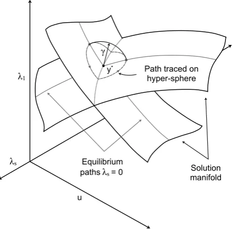
Fig. 3. Two equilibrium surfaces parametrised by a fundamental loading parameter,λ1, and a perturbing loading parameter,λs, intersecting to

produce a simple bifurcation. All equilibrium states of the unperturbed system within the vicinity of the bifurcation point,y∗_{, are determined by}

tracing the intersection of the solution manifold and a hypersphere describing a region around the bifurcation point.

primary path. For the simple case of a fundamental mechanical loading parameter,λ1, and a perturbation parameter,

λs, a perturbed equilibrium state is defined as follows:

F(y)≡F(u, λ1, λs)=f(u)−λ1pˆ1−λspˆs=0, (49)

wherepˆsis an arbitrary perturbing vector, not in the same direction as the fundamental loading vector,i.e.

ˆ

p1· ˆps

∥ ˆp1∥2·∥ ˆps∥2 ̸=

1. It is obvious from Eq.(49)that the unperturbed equilibrium equation is recovered forλs=0. The intersection of the two-dimensional solution manifold, described by Eq.(49), and a hypersphere of radiusγcentred around a bifurcation point, y∗ _{= (u}∗_{, λ}∗_{1,0), is a closed one-dimensional curve (see Fig. 3). This curve can be traced by defining the} hypersphere as an auxiliary equation,

G(y)≡

( _F(y)

(

y−y∗)⊤(

y−y∗)_−γ2 )

=0. (50)

This system can be solved via Newton’s method once a pertinent arc-length constraint,N(u, λ1, λs)=n⊤

uu+nλ1λ1+

n_λsλs−σ, is defined. Hence, by linearising Eq.(50) ⎡

⎢ ⎣

KT − ˆp1 − ˆps

2(

u−u∗)⊤

2(_λ1−λ∗

1 )

2λs

n⊤_u n_λ1 n_λs

⎤

⎥ ⎦

⎧

⎨

⎩ δu

δλ1 δλs

⎫

⎬

⎭ = −

⎧

⎪ ⎨

⎪ ⎩

F(u, λ1, λs)

(

y−y∗)⊤(

y−y∗) −γ2

N(u, λ1, λs)

⎫

⎪ ⎬

⎪ ⎭

. (51)

As this curve is followed, additional equilibrium solutions of the unperturbed system, either on a fundamental or bifurcated equilibrium path, are determined every timeλs changes sign (an approximate solution to λs = 0 can be determined by linear interpolation). Due to the fact that this curve connects solutions on adjacent, yet distinct equilibrium curves, it is often called abranch-connecting path.

In an analogous way to Crisfield’s spherical and cylindrical arc-length constraints [76], Eriksson [40] reports that the simplified cylindrical auxiliary equationg=(u−u∗₎⊤₍

u−u∗_)−γ2_{performs more robustly than the spherical}

The advantage of the branch-connecting approach is that the computational expense is basically the same no matter how many additional equilibrium paths exist. Furthermore, the same algorithm can also be used to determine the broken-away curve of a broken pitchfork bifurcation. In fact, the method can generally be used to uncover adjacent equilibrium paths that do not intersect with a primary loading path.

2.3.2. General foldlines

Path-following of foldlines could be posed as a general two-parameter problem with target parameters Λt =

(λt1, λt2),Λt ⊂ Λ. In a structural mechanics setting, however, our main interest is to compute the sensitivity

of critical points on a fundamental load–displacement path with respect to an added parameter. The equilibrium equations,F(u, λ1, λs,Λc)=0, are therefore written in terms of the active parametersλ1andλs—the former being

a fundamental loading parameter (thermal or mechanical), and the latter parametrising a secondary loading, a change in geometry or a variation in constitutive properties. The baseline problem corresponds to the baseline secondary parameter,λs = λb

s, and all other parameters,Λc ⊂ Λ, that define the problem are held constant at their baseline

values. The choice of secondary parameter,λs∈Λs, can be changed one at a time, such that a system with parameters

p>2 is framed as a collection of individual problems, each with p=2.

Depending on the nature ofλ1 (mechanical or thermal loading) and λs (secondary loading or changes to the structure), the equilibrium equations can be written in one of three forms as defined by Eqs.(21)–(23). The foldline algorithm then constrains the equilibrium equations to a curve that unfolds a baseline singular point with respect to another parameter,i.e.a curve describingλ∗₁ =λ∗₁(λs). The unfolding of limit and bifurcation points often results in a sequence of singular points of the same nature, limit and bifurcation, respectively. For the classic pitchfork bifurcation of the elastica, however, small geometric imperfections can break the pitchfork, thereby transforming the bifurcation point into a limit point. This means that for specific values of the secondary parameter, the unfolding of limit and bifurcation points can lead to sequences of singular points of the opposite nature. The foldline algorithm presented in this section can handle both types of singular points, such that sequences of limit points only, bifurcation points only and combinations of limit and bifurcation points can be traced.

In the present computational implementation both the nullvector and minimally augmented methods (see Section2.2.4) are used to formulate the auxiliary singularity condition required to trace along a foldline. The difference to the pinpointing procedure for individual singular points is thatλs is now introduced as a second parameter to be varied. This means that an additional equation needs to be specified to uniquely solve the system. As with all path-following techniques, this equation takes the form of a path-path-following constraint, and either Crisfield’s cylindrical [76] or Riks’ hyperplane constraint [47] may be used for this purpose. In general, the arc-length constraint may be written asN(u, λ1, λs)=n⊤_uu+n_λ1λ1+n_λsλs−σ, whereσis a constant that constrains the arc-length.

For the nullvector method, the general augmented system of Eq.(7)reduces to

GN(u, λ1, λs,Λc,φ)≡ ⎛

⎜ ⎜ ⎜ ⎝

F(u, λ1, λs,Λc)

KT(u, λ1, λs,Λc)φ ∥φ∥₂−1

N(u, λ1, λs)

⎞

⎟ ⎟ ⎟ ⎠

=0. (52)

Eq.(52)features (2n+2) equations in (2n+p) variables, and the (p−2) extra equations required to solve the system are implicit in the definition that the parametersΛcare held constant,i.e.Λcj =Σj for j =3. . .p. Starting from a

singular state, (u∗_{, λ}∗

t,Λ

∗

c), with associated critical eigenvector,φ, on a fundamental equilibrium path of the baseline

problem,λs=λb_s, a locus of singular points is continued using Newton’s method,

⎡ ⎢ ⎢ ⎢ ⎢ ⎢ ⎣

KT F,λ1 F,λs 0 (KTφ)_,u (KTφ)_,λ1 (KTφ)_,λs KT

01×n 0 0 φ

⊤

∥φ∥₂

n⊤_u n_λ1 n_λs 01×n

⎤ ⎥ ⎥ ⎥ ⎥ ⎥ ⎦ ⎧ ⎪ ⎪ ⎨ ⎪ ⎪ ⎩ δu δλ1 δλs δφ ⎫ ⎪ ⎪ ⎬ ⎪ ⎪ ⎭ = − ⎧ ⎪ ⎪ ⎪ ⎨ ⎪ ⎪ ⎪ ⎩

F(u, λ1, λs,Λc)

KT(u, λ1, λs,Λc)φ ∥φ∥₂−1

N(u, λ1, λs)

⎫ ⎪ ⎪ ⎪ ⎬ ⎪ ⎪ ⎪ ⎭ . (53)

Approximate directional derivatives of the tangential stiffness matrix,KT, are computed using Eqs.(36)and(37).

mechanical load vectors, − ˆp1 and− ˆps, respectively, then approximate directional derivatives are computed using

Eq.(38).

In the same manner, the secondary parameter,λs, is introduced into the minimally augmented system of Eq.(42), and the system further augmented using an arc-length constraint. Hence,

GN(u, λ1, λs,Λc)≡ ⎛

⎝

F(u, λ1, λs,Λc) µ(u, λ1, λs,Λc)

N(u, λ1, λs)

⎞

⎠=0, (54)

which defines (n+2) equations in (n+p) variables with the (p−2) extra equations being implicit in the definition that control parametersΛcare constants. Linearisation of Eq.(54)gives

⎡

⎢ ⎣

KT F,λ1 F,λs µ⊤

,u µ,λ1 µ,λs

n⊤_u n_λ1 n_λs

⎤ ⎥ ⎦ ⎧ ⎨ ⎩ δu δλ1 δλs ⎫ ⎬ ⎭ = − ⎧ ⎨ ⎩

F(u, λ1, λs,Λc) µ(u, λ1, λs,Λc)

N(u, λ1, λs)

⎫

⎬

⎭

, (55)

where approximate directional derivatives of the scalar singularity equation are computed using Eqs.(44)and(45). When either λ1 or λs are displacement-independent mechanical loading parameters, µ_,λ1 = 0 and µ_,λs = 0, respectively, and the directional derivativesF_,λ1 = − ˆp1andF,λs = − ˆps. Otherwise,F,λ1 andF,λs are approximated

using Eq.(38). As described in Section2.2.4, the eigenvalue,µ, and eigenvector,φ, need to be updated at the end of every iteration of Eq.(55)using the iterative eigenvalue problem in Eq.(41).

To solve the nullvector and minimally augmented systems of Eqs.(53)and(55)efficiently, a partitioning procedure is utilised such that only the tangential stiffness matrix needs to be factorised. The partitioning procedure is entirely algebraic (as shown inAppendix), and for a more detailed incremental–iterative bordering algorithm the interested reader is directed to Moghaddasie & Stanciulescu [99] and Rezaiee-Pajand & Moghaddasie [100].

2.3.3. Foldlines of bifurcation points

In some cases, it is useful to constrain the foldline solver purely to bifurcation points,e.g.when foldlines of limit and bifurcation points intersect and we want to prevent the solver from jumping from one curve to the other. To explicitly constrain the solver to symmetry-breaking bifurcation points, the equilibrium equations are perturbed by a vectorϕthat is antisymmetric with respect to the symmetry in the displacement vectoru[44]. The perturbing vector ϕremains constant throughout the iterations of a foldline increment, and is chosen as the nullvector of the previously converged increment along the foldline. The magnitude of the asymmetry is controlled by a scalar variable,τ, and the additional equationh = u⊤_{φ = 0 enforces orthogonality of the displacement vector and nullvector throughout the} equilibrium iterations. The unperturbed equilibrium equations are recovered forτ =0, and this is input as an initial predictor to start the equilibrium iterations. In our experience,τrarely exceeds 10−7_{throughout the iterative corrector}

procedure.

The set of coupled equations, describing a foldline of bifurcation points using the nullvector method, is

GN(u, λ1, λs,Λc,φ, τ)≡ ⎛ ⎜ ⎜ ⎜ ⎜ ⎜ ⎜ ⎝

F(u, λ1, λs,Λc)+τϕ

KT(u, λ1, λs,Λc)φ ∥φ∥₂−1

u⊤φ

N(u, λ1, λs)

⎞ ⎟ ⎟ ⎟ ⎟ ⎟ ⎟ ⎠

=0, (56)

with the following linearised system used in Newton’s method:

⎡ ⎢ ⎢ ⎢ ⎢ ⎢ ⎢ ⎢ ⎢ ⎣

KT F_,λ1 F_,λs 0 ϕ (KTφ)_,u (KTφ)_,λ1 (KTφ)_,λs KT 0n×1

01×n 0 0

φ⊤

∥φ∥₂ 0

φ⊤

0 0 u⊤ 0

n⊤_u n_λ1 n_λs 01×n 0

⎤ ⎥ ⎥ ⎥ ⎥ ⎥ ⎥ ⎥ ⎥ ⎦ ⎧ ⎪ ⎪ ⎪ ⎪ ⎨ ⎪ ⎪ ⎪ ⎪ ⎩ δu δλ1 δλs δφ δτ ⎫ ⎪ ⎪ ⎪ ⎪ ⎬ ⎪ ⎪ ⎪ ⎪ ⎭ = − ⎧ ⎪ ⎪ ⎪ ⎪ ⎪ ⎪ ⎨ ⎪ ⎪ ⎪ ⎪ ⎪ ⎪ ⎩

F(u, λ1, λs,Λc)+τϕ

KT(u, λ1, λs,Λc)φ ∥φ∥₂−1

u⊤φ

N(u, λ1, λs)

For the minimally augmented method, both the eigenvalue problem and the augmented equilibrium equations need to be perturbed. The perturbed iterative eigenvalue problem is

⎡

⎢ ⎣

−KT φk u φ⊤

k 0 0

u⊤ 0 0 ⎤ ⎥ ⎦ ⎧ ⎨ ⎩

φk+1 µk+1

hk+1 ⎫ ⎬ ⎭ = ⎧ ⎨ ⎩ 0 1 0 ⎫ ⎬ ⎭ , (58)

where pre-multiplication of the first row,KTφk+1 = µk+1φk +hk+1u, byφ⊤k+1 and application of the second row,

φ⊤

kφk+1 = 1, and third row,u⊤φk+1 = 0, returns the scalar condition µk+1 = φ⊤k+1KTφk+1. Eq.(58)is solved

efficiently using a partitioning procedure, by first computing immediate vectorsρ = K−_T1φ_k andν = K_T−1u, then

back-substituting to findµk+1= 1 φ⊤

k(ρ−ν

u⊤_ρ u⊤_ν)

andhk+1= −u ⊤_ρ

u⊤_νµk+1, and finally computingφk+1=µk+1ρ+hk+1ν.

Note thatudoes not change in Eq.(58)because the state, (u, λ1, λs), is updated in a separate iterative procedure of the augmented equilibrium equations. These augmented equilibrium equations are

GN(u, λ1, λs,Λc, τ)≡ ⎛

⎜ ⎜ ⎜ ⎝

F(u, λ1, λs,Λc)+τϕ µ(u, λ1, λs,Λc)

u⊤φ

N(u, λ1, λs)

⎞

⎟ ⎟ ⎟ ⎠

=0, (59)

which are solved in the following manner using Newton’s method,

⎡

⎢ ⎢ ⎢ ⎣

KT F,λ1 F,λs ϕ µ⊤

,u µ,λ1 µ,λs 0

φ⊤

0 0 0

n⊤_u n_λ1 n_λs 0

⎤ ⎥ ⎥ ⎥ ⎦ ⎧ ⎪ ⎪ ⎨ ⎪ ⎪ ⎩ δu δλ1 δλs δτ ⎫ ⎪ ⎪ ⎬ ⎪ ⎪ ⎭ = − ⎧ ⎪ ⎪ ⎪ ⎨ ⎪ ⎪ ⎪ ⎩

F(u, λ1, λs,Λc)+τϕ µ(u, λ1, λs,Λc)

u⊤φ

N(u, λ1, λs)

⎫ ⎪ ⎪ ⎪ ⎬ ⎪ ⎪ ⎪ ⎭ . (60)

The eigenvalue, µ, and eigenvector, φ, are updated at the end of every iteration of Eq. (60) using the iterative eigenvalue problem in Eq.(58).

All directional derivatives in the augmented systems Eqs. (57) and (60) are calculated using the expressions referenced in the previous section, and are again solved efficiently using an algebraic partitioning procedure (see

Appendix). For this purpose, the bordering algorithm presented in Refs. [44,99,100] may also be used as a template.

2.3.4. Tangent vectors to curves

The evaluation of the tangent space is important for predicting the direction of new solutions along a solution path. In a multi-parametric setting, the tangent space can also be used to determine the direction of greatest descent,i.e.the parameter or combination of parameters that has the greatest effect on the load-carrying capacity. The tangent space,

T, of the general augmented system,G(y) = 0, as defined in Eq.(6), is given by the nullspace of the differential matrix,

G_,yT=0. (61)

The dimension ofTdepends on the number of equations and the number of variables,y, in the augmented system,

G(y). As outlined in Section2.1,Ggenerally describes a system ofnequilibrium equations andrauxiliary equations in (n +q + p) variables (n degrees-of-freedom, q auxiliary variables and p parameters). In this general setting, the nullspace is (q+ p−r)-dimensional. For the one-dimensional subset curves studied here, however, we define

r =q+p−1 such that the nullspace is typically one-dimensional and therefore describes the tangent direction to the subset curve. At a singular point the nullspace may be of higher dimension due to the singularity ofKTwithinG,y,

such that the direction of the curve is not unique,e.g.two or more tangent directions at a bifurcation point.

First, we address the case of non-critical subset curves (q =0) with possibly more than one parameter (p ≥ 1). The tangent space is now a function ofy=(u,Λ) and defined by the differential matrix of Eq.(5):

G_,yT≡ [

KT F,Λ

g_,u g,Λ

] {

τu τΛ

}