Ant´onio Morgado1, Paulo Matos1, Vasco Manquinho1, and Jo˜ao Marques-Silva2
1
IST/INESC-ID, Technical University of Lisbon, Portugal
{ajrm, pocm, vmm}@sat.inesc-id.pt
2
School of Electronics and Computer Science, University of Southampton, UK
Abstract. This paper addresses the problem of counting models in in-teger linear programming (ILP) using Boolean Satisfiability (SAT) tech-niques, and proposes two approaches to solve this problem. The first approach consists of encoding ILP instances into pseudo-Boolean (PB) instances. Moreover, the paper introduces a model counter for PB con-straints, which can be used for counting models in PB as well as in ILP. A second alternative approach consists of encoding instances of ILP into instances of SAT. A two-step procedure is proposed, consisting of first mapping the ILP instance into PB constraints and then encoding the PB constraints into SAT. One key observation is that not all existing PB to SAT encodings can be used for counting models. The paper pro-vides conditions for PB to SAT encodings that can be safely used for model counting, and proves that some of the existing encodings are safe for model counting while others are not. Finally, the paper provides ex-perimental results, comparing the PB and SAT approaches, as well as existing alternative solutions.
1
Introduction
Besides its well-known theoretical relevancy, the problem of counting models of Boolean Satisfiability (SAT) formulas (#SAT) has a large number of key applica-tion areas [2,18]. Recent years have seen significant improvements in algorithms for #SAT, which include the utilization of well-known SAT techniques as well as the identification of connected components and component caching, but also variable lifting and blocking clauses [6,12,17,18]. Nevertheless, model counting is also extremely important in non-Boolean domains, including Integer Linear Pro-gramming (ILP) [5,11] and Linear Integer Arithmetic (LIA) [7,16]. This paper focus on ILP, but the techniques proposed can be extended to LIA.
Existing algorithms for counting models in ILP [5,11] are extremely sensi-tive to the number of variables in the problem formulation, being able to solve instances with a very small number of variables. Hence, in many practical ap-plications, existing algorithms are ineffective.
This paper proposes two alternative solutions to counting models in ILP, by considering the utilization of SAT-based techniques. The first approach consists of encoding instances of ILP into instances of pseudo-Boolean (PB) constraints.
A. Biere and C.P. Gomes (Eds.): SAT 2006, LNCS 4121, pp. 410–423, 2006. c
Moreover, the paper introduces a model counter for PB constraints, which can be used for counting models in PB as well as in ILP. A second alternative approach consists of encoding instances of ILP into instances of SAT. A two-step procedure is proposed, consisting of first mapping the ILP instance into PB constraints and then encoding the PB constraints into SAT. One key concern is that not all existing PB to SAT encodings can be used for counting models. The paper provides conditions for encodings that can be safely used for model counting, and proves that some of the existing PB to SAT encodings are safe for model counting. Finally, the paper provides experimental results, comparing the PB and the SAT approaches, as well as existing alternative solutions. The results provide interesting insights into the problem of counting models in ILP. First, the PB counter, albeit a preliminary prototype, is competitive with SAT counters, which integrate more sophisticated techniques including the identification of connected components and component caching. Second, the very effective SAT-techniques used in Cachet [18] may not scale for integer domains.
The paper is organized as follows. Section 2 presents the notation used through-out the paper. Afterwards, the paper addresses the encoding of ILP into PB con-straints, and describes a model counter for PB formulations. Section 5 details the second approach to model counting in ILP, based on encoding ILP into SAT. This section proves that some existing encodings will yield correct results, whereas oth-ers can overestimate the number of integer models. Section 6 compares the two ap-proaches and also evaluates an alternative solution [11]. Section 7 surveys related work, and the paper concludes in Section 8.
2
Definitions
An Integer Linear Programming (ILP) problem with n variables and m con-straints can be defined as follows [14]:
n
j=1
aijxj ≤bi,
xj, aij, bi∈
j∈ {1, . . . , n}, i∈ {1, . . . , m}
(1)
whereaijdenote the coefficients of the problem variablesxjin the set ofmlinear
In a propositional formula, a literal lj denotes either a variable xj or its
complement ¯xj. If a literallj =xj andxj is assigned value 1 orlj= ¯xj and xj
is assigned value 0, then the literal is said to be true. Otherwise, the literal is said to be false.
A propositional clause is a disjunction of literals such asl1∨l2∨. . .∨lkwhere
lj is a literal representing either xj or ¯xj. We should observe that propositional
clauses can also be represented as linear inequalities, e.g. kj=1lj ≥ 1. One
can obtain a linear inequality as in (1) if we replace literals ¯xj by 1−xj. In the
context of SAT we will represent propositional clauses as a disjunction of literals, instead of linear inequalities. However, in the context of ILP or pseudo-Boolean, we use the linear inequalities formalism.
Whenever an assignment toallproblem variables is found such that all prob-lem constraints become satisfied, we say that a model has been found. However, it may occur that apartial assignment(i.e. not all problem variables are assigned) is able to satisfy all problem constraints. In this case, the partial assignment represents a set of models for the problem instance.
We say that an ILP instance defines aconvex polytopeif the number of integer solutions (models) to the ILP constraints is finite. Note that all PB and SAT problem instances define rational convex polytopes since the value of the problem variables is bounded. Hence, the number of solutions isO(2n) for both PB and
SAT instances, where n is the number of problem variables. However, not all ILP instances define convex polytopes. For example, the following ILP has an infinite number of solutions:
x1−x2≤10, x1−x3≤5 x1, x2, x3∈
(2)
In section 3 we discuss how to determine if a set of ILP constraints define a convex polytope by finding lower and upper bounds on the value of all problem variables.
3
Encoding ILP into Pseudo-Boolean
This section presents a procedure to encode an Integer Linear Programming (ILP) problem instance into a Linear Pseudo-Boolean (PB) problem instance. The re-sulting PB instance can then be solved using specific Boolean techniques [1,8]. A key aspect of this encoding is to determine lower and upper bounds on the possible values of the integer valued variables in the ILP. We assume that the ILP instance defines a convex polytope; otherwise the number of integer solutions would be in-finite. Hence, every integer variable is guaranteed to have a lower and an upper bound.
Given an ILP instance as presented in section 2, letlower(xj) andupper(xj)
denote respectively the lower and upper bound on the value of variablexj in the
ILP. If specified in the problem instance, the values oflower(xj) andupper(xj)
In general, the lower and upper bounds of an integer valued variablexj can
be determined by solving a linear programming relaxation (LPR) as follows:
minimize/maximizexj
subject to
n
j=1
aijxj≤bi,
xj∈, aij, bi∈
(3)
where we useminimize ormaximizedepending on whether we are interested in obtaining a lower or a upper bound, respectively. Note that in this formulation all problem variables are no longer integer and there are known polynomial time algorithms for solving these formulations [14].
Letzm
j andzMj denote respectively the solutions of (3) in the minimization and
maximization formulations. By relaxing the variable integer constraints we can obtain a lower and upper bound on the value ofxj, since no integer solution to (1)
can be obtained such thatxj < zjm or xj > zjM. Hence, we have lower(xj) =
zjmandupper(xj) =zjM , wherez m
j denotes the smallest integer value not
lower thanzmj andzjM denotes the largest integer value not higher thanzjM. Observe that in order to obtain lower bounds on the problem variables, the well-known replacement of each problem variablexj withx
j−x
j, wherex
j ≥
0 and xj ≥ 0, cannot be used. For example, suppose we have the following constraints for variablex1:
x1≥ −1, x1≤3 (4)
In this formulation,x1is clearly bounded. However, if we replacex1withx1−x1, we would get:
x1−x1 ≥ −1, x1−x1 ≤3
x1≥0, x1 ≥0 (5)
For this new formulation, both variablesx1 and x
1 are not bounded, since we can always find arbitrary large values for x1 and x1 such that the constraints are satisfied.
One should also note that if (3) is unbounded for any given problem variable xj, then the original ILP does not define a convex polytope. Otherwise, if (3) is
bounded for all problem variables, then the ILP is a convex polytope and there is a finite number of integer solutions to (1).
Since all integer variablesxjof (1) are limited betweenlower(xj) andupper(xj)
in a convex polytope, we can apply a substitution of all variablesxj with yj −
lower(xj) so that in the new ILP we have all new problem variablesyjbounded
between 0 andupper(yj) whereupper(yj) =upper(xj)−lower(xj). Afterwards,
we can encode each integer variableyj as a set of weighted bits as follows:
yj= bj
i=0 2iyi
j
yi
j∈ {0,1}
wherebj is the number of bits necessary to representupper(yj) and variablesyji
are Boolean. Additionally, we can also add the following constraints:
bj
i=0
2iyji ≤upper(yj) (7)
As a result of integer variable replacements from (6) and the addition of upper bound constraints from (7), we get a pseudo-Boolean instance that encodes the convex polytope defined by the original ILP.
It is important to ensure that the number of solutions of the PB instance is the same as in the original ILP. Indeed, for this encoding, every unique satisfiable assignment for the ILP instance corresponds to a unique satisfiable assignment for the PB instance, because the integer variables are encoded as a set of weighted bits as it is represented in the computer memory.
4
Model Counting in Pseudo-Boolean Formulations
One way for performing model counting in Pseudo-Boolean (PB) formulations is to implicitly enumerate all possible variable assignments using a backtrack search PB solver. Moreover, current state-of-the-art PB solvers are able to perform con-flict learning[1,8] and thus prevent entering areas of the search space where no satisfiable assignment exists. This technique has been found particularly useful when the solver has to implicitly visit the complete search space.
It is possible to modify backtrack search PB solvers to count models in PB formulations. Basically, whenever a new solution is found, a propositional clause is added such that it prevents accounting for the same solution later in the search. In the context of model counting, these clauses are known as blocking clauses[12,17].
The most straightforward way of generating a new blocking clause is to con-sider the negation of the search path when a new satisfiable assignment is found. Therefore, if the search path corresponds to the decision assignments {x1=v1, x2=v2, . . . , xk=vk}, then the blocking clause is defined by:
k
j=1
lj≥1 (8)
wherelj=xjifxj = 0 in the search path orlj= ¯xj ifxj = 1. Observe that this
Simplification of Satisfying Partial Assignments.It is well-known that the problem of computing the satisfying partial assignment with the smallest num-ber of specified variables can be formulated as an integer linear program [15]. However, we are just interested in simplifying satisfying partial assignments com-puted by a PB solver.
Variable lifting denotes a number of techniques used for the elimination of assignments that can be declared redundant [12,17]. A simple variable lifting technique consists of removing from a satisfying partial assignment all variable assignments that are not used to satisfy any constraint. Moreover, these vari-able assignments cannot also be used in constraints that imply other varivari-able assignments. When using this technique, we can immediately conclude that all implied assignments cannot be removed from the partial assignment since they are necessary to satisfy at least one constraint. Otherwise, these assignments would not be implied. Hence, we only have to check decision assignments.
Suppose we have the following decision assignment x1 = x2 =x3 = 0 and thatx5= 0 is an implied assignment. Consider also the following constraints:
(x1+x2+x3≤1)∧(x2+x3≤1)∧(x2+x4≤1)∧(−x3+x5≤0) (9)
Clearly, the assignment tox1 is not relevant to satisfy the problem constraints. Note that x3 cannot be considered irrelevant, since it is necessary to imply the value of x5. Hence, the resulting blocking clause would be x2+x3 ≥ 1. Since there are two variables (x1 and x4) that are not relevant to satisfy the constraints in this partial assignment, then we conclude that 4 models have been found. In [12,17] other lifting techniques are presented. However, they require a significant computational overhead.
Additional SAT Techniques. The identification of connected components [6] and component caching [18] are among the most effective techniques for model counting instances of SAT. These techniques are not yet integrated in the PB model counter described above, since they will require significant re-implemen-tation effort, and our objective is first to evaluate whether these techniques are effective for ILP and PB model counting.
5
Encoding Pseudo-Boolean Constraints as SAT
Definition 1 (Counting Safety).A PB formulation to SAT encoding is count-ing safe iff the number of models in the PB formulation and in the encoded SAT formulation are the same.
5.1 Unsafe Encodings
The vast majority of PB to SAT encodings solely aim the discovery of one solution and may introduce auxiliary variables. These variables may lead to double counting of the same solution in pseudo-Boolean. For example, consider the following PB constraints:
2x0+ 4x1+ 8x2+ 3y0+ 6y1+ 12y2≤18 −2x0−4x1−8x2+ 1y0+ 2y1+ 4y2≥ −10
If any of the encodings proposed in [9] is used with this example, and the re-sulting CNF formula is given to model counter, e.g.cachet [18], the number of models reported will be at least 38. However, the correct number of models for this example is 31. Hence, the encodings proposed in [9] do not satisfy the count-ing safety property, and cannot be used for model countcount-ing. The next section addresses encodings which are counting safe.
5.2 Safe Encodings
Both the well-known Warners PB to SAT encoding [19] as well as the more recent arc-consistency encoding of Bailleux, Boufkhad and Roussel (BBR) [4] can be shown to be counting safe. Due to space constraints, this section addresses solely the BBR encoding; a detailed analysis of Warners encoding is available in [13]. Next, we provide a brief description of the BBR PB to SAT encoding [4].
Consider a pseudo-Boolean constraintω with the constraint literalslj sorted
according to their coefficientsaj:
ω=
n
j=1
ajlj ≤b,
where 0< a1≤a2≤. . .≤an
(10)
Letωi,krepresent the constraintωconsidering only the firstiliterals (0≤i≤n)
with the right-hand side valuek, i.e.ωi,k :
i
j=1ajlj ≤k. Therefore, the original
constraintω corresponds toωn,b.
In order to generate the CNF encoding for a given constraintω, we need to introduce new Boolean variables Di,k which represent the satisfaction of
con-straints ωi,k obtained from ω. Hence, we have Di,k = 1 iff constraint ωi,k is
satisfied. As a result,Dn,b= 1 represents the satisfaction of the original
pseudo-Boolean constraintωin the CNF encoding.
When building the CNF encoding, variablesDi,k are said to be terminal if
The CNF encoding for a pseudo-Boolean constraintω proceeds as follows:
1. Start with a set of variables containing variablesxjin constraintω, as well as
variableDn,b, and an empty set of propositional clauses. Mark all variables
xj.
2. Consider an unmarked variableDi,k.
3. IfDi,kis a non-terminal variable, add two new variablesDi−1,kandDi−1,k−ai
to the set of variables, if they are not already in this set. Moreover, mark se-lected variableDi,k and add the following propositional clauses:
¯
Di−1,k−ai+Di,k≥1 (11)
¯
Di,k+Di−1,k≥1 (12)
¯
Di,k+ ¯li+Di−1,k−ai≥1 (13)
¯
Di−1,k+li+Di,k≥1 (14)
4. IfDi,k is a terminal variable, and ifk= 0, then:
Di,k=
⎧ ⎨ ⎩
0 ifk <0.Add ¯Di,k≥1 to the clause set.
1 if
i
j=1
aj≤k.AddDi,k≥1 to the clause set. (15)
Otherwise, ifk= 0, then add the following set of clauses:
¯
Di,k+ ¯lj≥1,1≤j≤i (16) i
j=1
lj+Di,k≥1 (17)
5. If there are any unmarked variables, go to step 2. Otherwise, the proposi-tional clause set contains the CNF encoding of constraintω and the proce-dure terminates.
The following example illustrates how the proposed CNF encoding works:
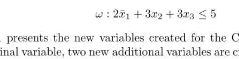
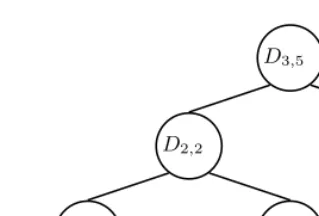
[image:8.513.98.341.510.570.2]ω: 2¯x1+ 3x2+ 3x3≤5 (18)
Figure 1 presents the new variables created for the CNF encoding. For each non-terminal variable, two new additional variables are created whereas terminal variables are represented as leaf nodes. The full encoding for constraintω as a set of propositional clauses is as follows:
D3,5≥1 D1¯ ,−1+D2,2≥1 D1¯ ,−1≥1 ¯
D2,2+D3,5≥1 D2¯ ,2+D1,2≥1 D1,2≥1 ¯
D3,5+D2,5≥1 D2¯ ,2+ ¯x2+D1,−1≥1 ¯
D3,5+ ¯x3+D2,2≥1 ¯D1,2+x2+D2,2≥1 ¯
D2,5+x3+D3,5≥1D2,5≥1
(19)
D1,−1 D1,2
[image:9.513.128.288.52.160.2]D2,2 D2,5 D3,5
Fig. 1.Additional variables in CNF encoding
This is required since D3,5 represents the satisfaction of the original pseudo-Boolean constraint.
Finally, we refer to [4] for details, namely proofs of correction of the encoding and of the maintenance of generalized arc consistency in the resulting CNF encoding, as well as examples of constraints for which this encoding provides exponential increase in the size of the CNF encoding.
Theorem 1. The BBR arc-consistency encoding [4] is counting safe.
Proof:
We want to prove that to each model for the PB constraints there is a corre-sponding unique model for the SAT encoding, and that to each model for the SAT encoding there is a unique corresponding model for the PB constraints.
(←) If we have a model for the SAT encoding then we can only have one model for the PB constraints, which is the model for the SAT encoding restricted to the variables for the PB constraints.
(→) Suppose we have a model for the PB constraints. We know that the encoding is correct [4], so we already know that there exists at least one model for the SAT encoding corresponding to the model for the PB constraints. What we want to show is that this model is unique. We also know that the model in SAT corresponds to the same assignments made to the variables of the PB constraints plus the assignments to the variables introduced by the encoding. In order to show that the model is unique all we have to prove is that these new variablesDi,b can only have one possible assignment for satisfying the created
instance. We are going to prove this claim by induction onn. Let us first consider a PB constraintnj=1ajxj≤kand the corresponding variable nodeDn,k.
Base:n= 1:
There can be two cases, depending on whether D1,k is terminal. If D1,k is
ter-minal we may havek= 0 ork= 0. Ifk= 0, due to the definition of a terminal node, eitherk <0 and the value ofD1,k is 0, ora1≤kand the value ofD1,kis
1. Otherwise, ifk= 0, then the encoding adds clauses ( ¯D1,0 ∨ x1), (D1,0 ∨ x1).¯ Sincex1 has a determined value it implies the unique value ofD1,k.
We now consider the case whenD1,kis not terminal. In this case, the encoding
and ( ¯D0,k ∨ x1 ∨ D1,k). Since D1,k is not terminal, then if k > 0 we have
D0,k = 1 or if k < a1 we haveD0,k−a1 = 0. The first and the second clauses
added by the encoding are trivially satisfied. By removing the false literals of the third and fourth clauses we get ( ¯D1,k ∨ x1), (x1¯ ∨ D1,k). Sincex1 has a
determined value both clauses imply the unique value ofD1,k.
Step:
Hypothesis: Fori < n, Di,b has only one possible assignment that satisfies the
created instance.
We now consider node Dn,k. If the node is terminal with k < 0, then the
encoding adds the clause ( ¯Dn,k) andDn,k can only be assigned value false.
If the node is terminal withk= 0 andk≥nj=1aj, then the encoding adds
the clause (Dn,k) andDn,k can only be assigned value true.
If the node is terminal with k = 0, then the encoding adds the clauses ( ¯Dn,0 ∨ x¯j), 1 ≤j ≤n and (x1∨x2∨. . .∨xi∨Dn,0). Two situations may
occur. If all the variablesxj, 1≤j ≤n, are false, then (17) implies the value of
Dn,0 to true. If at least onexj, 1≤j≤nis true, then (16) implies the value of
Dn,0 to false andxj satisfies (17).
If the node is non-terminal, then we apply the hypothesis toDn−1,k and to
Dn−1,k−an−1. We get that these variable nodes have a fixed known value. We
have four cases depending on the value of the variable nodes:
– IfDn−1,k and Dn−1,k−an−1 are false, then from (12) Dn,k can only be false
and the other clauses are all satisfied.
– IfDn−1,k is false andDn−1,k−an−1 is true, then from (11) and (12) there is
a contradiction, and the encoded instance is unsatisfiable. This situation is acceptable since we cannot have (nj=1−1ajxj ≤k−an−1) being satisfiable
and at the same time being unable to satisfy the same left hand side of the equation with a higher right hand side (nj=1−1ajxj≤k).
– IfDn−1,k is true andDn−1,k−an−1 is false, then we can have two cases:
xn is false , then from (14)Dn,k can only be true and the other clauses are
all satisfied;
xn is true , then from (13)Dn,k can only be false and the other clauses are
all satisfied.
– If Dn−1,k = 1 and Dn−1,k−an−1 = 1, then from (11)Dn,k = 1 and all the
other clauses are satisfied.
Finally, the results holds for any constraint, and so necessarily holds for all constraints in an instance of PB.
6
Experimental Results
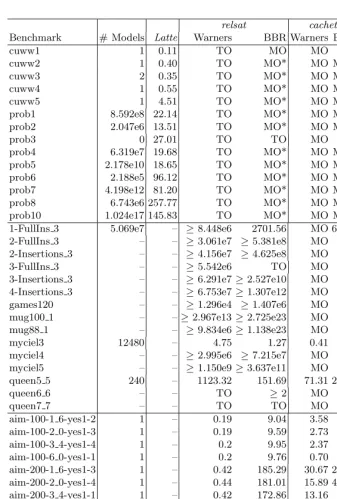
to use the SAT model counters, we use the counting safe encodings of Warn-ers [19] as well as the arc-consistency encoding proposed by Bailleux, Boufkhad and Roussel (BBR) [4]. All CPU times presented are for a AMD Athlon 1.9GHz processor with 1GB of physical memory. The time limit for each instance was set to one hour. If the time limit was reached, we provide a partial solution when one is available, i.e. the number of models found when the search was stopped. This is preceded by the sign≥since the total number of models must be higher than or equal to the ones already found. If all models are found, we provide the total time in seconds. In cases where time limit was reached and the counter did not provide any count of the number of models,TO(Time Out) is shown. All processes were run with 900MB of allowed memory.MO (Memory Out) is shown for the cases where the counter reached the allowed memory limit. On some instances of Table 1MO* is shown because it was the translator of pseudo-Boolean to SAT that reached the memory limit instead of the counter. Observe thatMO*can only take place with the BBR encoding.
The experimental results are shown in Table 1, and are organized in three parts, according to the source of the problem instances. The first part of Table 1 presents results for instances of finding theFrobeniusnumber plus 1 in knapsack problems [11]. For these instances, Latte is the only solver able to count the number of models. The underline numerical problem proved to be very difficult for pseudo-Boolean or SAT counters. Nevertheless, our solver pb counter was able to find partial solutions for some instances, while bothcachetandrelsat(in both encodings) were unable to do so.
Table 1.Results on several benchmark instances
relsat cachet
Benchmark # Models Latte Warners BBR Warners BBRpb counter
cuww1 1 0.11 TO MO MO MO TO
cuww2 1 0.40 TO MO* MO MO* TO
cuww3 2 0.35 TO MO* MO MO* TO
cuww4 1 0.55 TO MO* MO MO* TO
cuww5 1 4.51 TO MO* MO MO* TO
prob1 8.592e8 22.14 TO MO* MO MO* TO
prob2 2.047e6 13.51 TO MO* MO MO* TO
prob3 0 27.01 TO TO MO MO TO
prob4 6.319e7 19.68 TO MO* MO MO* TO
prob5 2.178e10 18.65 TO MO* MO MO* ≥4.337e4
prob6 2.188e5 96.12 TO MO* MO MO* ≥7
prob7 4.198e12 81.20 TO MO* MO MO* ≥3.812e4
prob8 6.743e6 257.77 TO MO* MO MO* TO
prob10 1.024e17 145.83 TO MO* MO MO* ≥764
1-FullIns 3 5.069e7 – ≥8.448e6 2701.56 MO 67.73 ≥5.194e6 2-FullIns 3 – – ≥3.061e7 ≥5.381e8 MO MO ≥1.067e7 2-Insertions 3 – – ≥4.156e7 ≥4.625e8 MO MO ≥9.006e6
3-FullIns 3 – – ≥5.542e6 TO MO MO ≥5.217e6
3-Insertions 3 – – ≥6.291e7≥2.527e10 MO MO ≥3.094e7 4-Insertions 3 – – ≥6.753e7≥1.307e12 MO MO ≥1.501e7
games120 – – ≥1.296e4 ≥1.407e6 MO MO ≥1.194e6
mug100 1 – –≥2.967e13≥2.725e23 MO MO ≥2.476e7
mug88 1 – – ≥9.834e6≥1.138e23 MO MO ≥1.513e7
myciel3 12480 – 4.75 1.27 0.41 0.26 0.96
myciel4 – – ≥2.995e6 ≥7.215e7 MO MO ≥5.065e6
myciel5 – – ≥1.150e9≥3.637e11 MO MO ≥1.134e7
queen5 5 240 – 1123.32 151.69 71.31 29.78 4.38
queen6 6 – – TO ≥2 MO MO ≥1.251e4
queen7 7 – – TO TO MO MO ≥1.447e3
aim-100-1 6-yes1-2 1 – 0.19 9.04 3.58 2.27 0.02
aim-100-2 0-yes1-3 1 – 0.19 9.59 2.73 2.61 0.03
aim-100-3 4-yes1-4 1 – 0.2 9.95 2.37 4.98 0.04
aim-100-6 0-yes1-1 1 – 0.2 9.76 0.70 1.31 0.05
aim-200-1 6-yes1-3 1 – 0.42 185.29 30.67 20.42 0.04 aim-200-2 0-yes1-4 1 – 0.44 181.01 15.89 41.97 0.07
aim-200-3 4-yes1-1 1 – 0.42 172.86 13.16 MO 0.08
aim-200-6 0-yes1-2 1 – 0.51 169.77 6.67 24.55 0.14
ii8a1 1056 – 17.41 45.77 18.67 7.35 7.25
jnh1 12 – 2.26 1079.66 7.52 8.12 0.53
jnh12 1 – 0.21 1.95 0.97 0.81 0.07
jnh17 35 – 0.42 6.13 1.19 2.49 0.20
jnh7 26 – 1.37 6.09 4.18 1.75 0.26
ssa7552-038 – – TO TO MO MO ≥1.853e4
7
Related Work
Besides the work on model counting and enumeration in SAT [6,12,17,18], there has been work on model counting in non-Boolean domains, including Integer Linear Programming (ILP) [5,11] and Linear Integer Arithmetic (LIA) [7,16].
Existing work on model counting in LIA is described in [7,16]. The work of [7] is based binary decision diagrams and does not scale to large number of variables. The work of [16] enumerates a large number of applications for model counting in LIA. The proposed algorithm is also only suitable for a small number of variables, or when most variables have fixed values.
The most well-known work on model counting in ILP is Barvinok’s algo-rithm [5]. An existing implementation,LattE [11], which incorporates a number of improvements, has been extensively used. As the results of Section 6 confirm, Barvinok’s algorithm is adequate for instances of ILP with a small number of variables which may have larger domains. Observe that the algorithms for model counting in LIA can also be used for ILP (a special case of LIA) but current solutions can only handle small instances.
8
Conclusions
This paper proposes two alternative approaches for counting models in ILP instances. The first approach is based on encoding ILP into Pseudo-Boolean (PB) and using a PB counter. A PB counter was developed for this purpose. A second approach is based on encoding ILP into SAT, using an intermediate encoding into PB. The paper shows that some PB to SAT encoding may overestimate the number of models, whereas others are shown to yield the correct number of models. As a result, counting models in integer domains can be achieved by encoding ILP constraints into SAT and directly using SAT model counters, thus taking advantage of the techniques already incorporated into SAT counters. Experimental results indicate that the PB counter is competitive with the SAT counters. Moreover, an existing alternative to SAT-based model counters, using Barvinok’s algorithm [5,11], provides essentially orthogonal results, being more efficient for problem instances having few variables with large domains, and being inadequate for problem instances having many variables with small domains.
Despite the interesting insights, many challenges still remain. The PB counter is a prototype, aiming to prove the concept of counting models for PB con-straints. A more sophisticated algorithm is expected to provide significant gains, for example if connected components are identified for PB constraints. There is also a clear gap betweenLattE (the implementation of Barvinok’s algorithm) and the SAT-based solutions. Work on closing this gap is also an interesting chal-lenge. Finally, the utilization of the model counter in instances of linear integer arithmetic [7,16], one of the motivations for this work, will require significantly more optimized ILP counters.
References
1. F. Aloul, A. Ramani, I. Markov, and K. Sakallah. Generic ILP versus specialized 0-1 ILP: An update. InInternational Conference on Computer-Aided Design, pages 450–457, November 2002.
2. F. Bacchus, S. Dalmao, and T. Pitassi. Algorithms and complexity results for #SAT and bayesian inference. InSymposium on Foundations of Computer Science, pages 340–351, 2003.
3. O. Bailleux and Y. Boufkhad. Full CNF encoding: The counting constraints case. In Seventh International Conference on Theory and Applications of Satisfiability Testing, 2004.
4. O. Bailleux, Y. Boufkhad, and O. Roussel. A translation of pseudo Boolean con-straints to SAT. Journal on Satisfiability, Boolean Modeling and Computation, 2, March 2006.
5. A. Barvinok and J. Pommersheim. An algorithmic theory of lattice points in polyhedra. InNew Perspectives in Algebraic Combinatorics, volume 38, pages 91– 147. MSRI Publications, Cambridge University Press, 1999.
6. R. J. Bayardo and J. D. Pehoushek. Counting models using connected components. InNational Conference on Artificial Intelligence, 2000.
7. B. Boigelot and L. Latour. Counting the solutions of presburger equations without enumerating them. Theoretical Computer Science, 313(1):17–29, 2004.
8. D. Chai and A. Kuehlmann. A Fast Pseudo-Boolean Constraint Solver. In Pro-ceedings of the Design Automation Conference, pages 830–835, 2003.
9. N. E´en and N. S¨orensson. Translating pseudo-Boolean constraints into SAT. Jour-nal on Satisfiability, Boolean Modeling and Computation, 2, March 2006.
10. D. S. Johnson and M. A. Trick. Second DIMACS Implementation Challenge. DIMACS Series in Discrete Mathematics and Theoretical Computer Science, 1994. 11. J. A. D. Loera, R. Hemmecke, J. Tauzer, and R. Yoshida. Effective lattice point counting in rational convex polytopes. J. Symb. Comput., 38(4):1273–1302, 2004. 12. K. L. McMillan. Applying SAT methods in unbounded symbolic model checking.
InInternational Conference on Computer-Aided Verification, 2002.
13. A. Morgado, P. Matos, V. Manquinho, and J. Marques-Silva. Counting models in integer domains. Technical Report 05/2006, INESC-ID, March 2006.
14. G. L. Nemhauser and L. A. Wolsey.Integer and Combinatorial Optimization. John Wiley & Sons, 1988.
15. C. Pizzuti. Computing Prime Implicants by Integer Programming. InProceedings of the International Conference on Tools with Artificial Intelligence, pages 332–336, November 1996.
16. W. Pugh. Counting solutions to presburger formulas: How and why. InConference on Programming Language Design and Implementation, pages 121–134, June 1994. 17. K. Ravi and F. Somenzi. Minimal satisfying assignments for conjunctive normal formulae. InInternational Conference on Tools and Algorithms for the Construc-tion and Analysis of Systems, 2004.
18. T. Sang, F. Bacchus, P. Beame, H. A. Kautz, and T. Pitassi. Combining com-ponent caching and clause learning for effective model counting. InInternational Conference on Theory and Applications of Satisfiability Testing, May 2004. 19. J. P. Warners. A linear-time transformation of linear inequalities into conjunctive