Digitizing signals a short tutorial guide

Introduction

Digitizing a signal is the first step in digital signal processing – get it wrong and all subsequent work may be wasted. We will discuss the principles underpinning this procedure, and some of the practical problems, and potential pitfalls along the way. The ECG (electrocardiogram) signal will be used to provide practical illustrations, and further examples from other biomedical signals are given at the end of this tutorial.

In analogue-to-digital conversion, or digitizing, an analogue signal is converted into digital format. Analogue signal have amplitudes that are known at every

instant in time, and can take on any value (usually limited by a minimum and maximum determined by the type of signal and the equipment used to acquire it). Clearly the ECG signal, as measured on the patient’s chest (fig. 1, top plot) and then amplified by the ECG system, falls within this definition. Digital signals, on the other hand, are given by a sequence of numbers that represent samples of the signals, as illustrated in fig. 1 (bottom plot). Digital signals can then be processed in ‘real-time’ (or on-line, i.e. simultaneously with acquisition), or stored for later ‘off-line’ processing and analysis by a computer. Essentially, any signal processing operation that can be performed on analogue signals can also be carried out on the digitized version, and in many cases more easily, cheaply, and flexibly. There

are also a number of operations that are readily applied on digital signals, that could not easily be implemented in analogue form (e.g. operations that require future, as well as past samples). Digital processing thus holds many practical advantages, and is progressively replacing analogue techniques.

The process of analogue-to-digital conversion involves a number of different stages, as illustrated in fig. 2. Each of these will now be considered, with particular attention to if and when information is lost by sampling.

Digitizing Signals – a Short

Tutorial Guide

David M. Simpson, Antonio De Stefano

Institute of Sound and Vibration Research, University of Southampton SO17 1BJ

Tel. 023 8059 3221 e-mail: ds@isvr.soton.ac.uk

Abstract

Converting the analogue signal, as captured from a patient, into digital format is known as digitizing, or analogue to digital conversion. This is a vital first step in for digital signal processing. The acquisition of high-quality data requires appropriate choices of system and parameters (sampling rate, anti-alias filter, amplification, number of ‘bits’). Thus tutorial aims to provide a practical guide to making these choices, and explains the underlying principles (rather than the mathematical theory and proofs) and potential pitfalls. Illustrative examples from different physiological signals are provided.

Figure 1. An ECG signal (analogue signal in the top plot), and the sampled version (digital signal,

The sampling theorem and aliasing

The ‘sampling rate’ is defined as the number of samples acquired, per unit time, and is usually given in samples/sec or Hz. It is intuitively clear that at a higher sampling rate, the digital signal provides a better approximation to the analogue signal. It may furthermore be shown from theory that if the sampling rate is sufficiently high, the analogue signal can be reconstructed exactly from the samples, i.e. there is no loss of information in the process of sampling. The sampling theorem states that this recovery of the analogue signal from its sampled version is possible, when the sampling rate is greater than twice the maximum frequency present in the signal. This provides the main criterion for selecting the sampling rate.

THE SAMPLING RATE MUST BE GREATER THAN TWICE THE MAXIMUM FREQUENCY PRESENT IN THE SIGNAL.

Thus, for example in fig. 1, the ECG signal had a maximum frequency of about 40 Hz (determined by the filter settings during acquisition, and confirmed by observing the spectrum), and was sampled at 100 Hz (i.e. > 2*40). The analogue signal (solid line) could therefore be reconstructed

perfectly from the samples (•)1_{. It would thus also be possible}

to calculate the samples corresponding to any other arbitrary sampling rate, from the digital signal acquired at 100 Hz.

When the sampling rate is lower than required, aliasing occurs, as illustrated in fig. 3. Consider a sine-wave of 1.5 Hz (fig. 3a), sampled at 8.5 Hz. According to the sampling theorem, this sampling rate is adequate, and the original sine-wave can be reconstructed from the samples. Now consider a 10 Hz sine-wave (fig. 3b), again sampled at

fs=8.5 Hz, i.e. much below the minimum of 20 Hz that is

required according to the sampling theorem. It may be noted, that the samples obtained are identical to those in fig. 3a, i.e. it would appear that the signal was made up of a sine-wave of 1.5 Hz, rather than one of 10 Hz. This change of frequency (from 10 to 1.5 Hz in this example) is known as aliasing. Sine-waves at 18.5 and 27 Hz also give identical digital signals (fig. 3c and d), and from these samples it would be impossible to determine which frequency was present in the original analogue signal. Only when the sampling theorem is obeyed, is there no ambiguity as to the frequency content of the signal.

Figure 2. The main steps in digital signal acquisition. The plots illustrate

the manner in which each step modifies the input.

Figure 3. Sine waves at 1.5 Hz, 10 Hz, 18.5 Hz, and 27 Hz, all give

exactly the same sample-values (marked as o), when sampled at 8.5 Hz. Thus, the sampled sine-waves of 10, 18.5 and 27 Hz appear to have been acquired from a 1.5 Hz sine-wave, i.e. they have been 'aliased' down to 1.5 Hz. In order to avoid this ambiguity as to the frequency in the analogue signal, the sampling rate must always be greater than twice the frequency present in the data.

1_{This reconstruction can be achieved by applying an analogue low-pass filter to the sampled signal, when each sample is}

represented by an impulse. This reconstruction process is clearly quite different from the simple linear interpolation between samples usually employed, when signals are plotted on a computer screen.

a

b

c

d

amplitude

amplitude

time (s)

time (s)

time (s)

time (s)

amplitude

If a signal has been sampled with a sampling rate that is too low and aliasing has arisen, it is (normally) impossible to restore the original data. The error cannot be undone and the signal should be discarded. Practical signals, such as the ECG, can be considered as made up of a sum of sine (and cosine) waves of different frequencies, in accordance

with Fourier analysis[1]_{. In order to adequately digitize such}

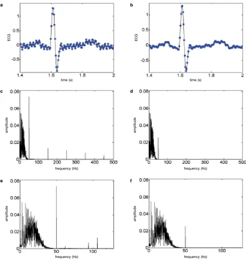
signals, the maximum frequency present in the signal must be considered, and a sampling rate that is more than twice this value must be chosen. In order to ensure a known upper limit to the frequency content of a signal, a low-pass filter (the anti-alias filter – see fig. 2) should be applied prior to sampling. For the example of the ECG signal, typically all the important information is contained in the band up to about 100 Hz. In the specific example below (fig. 4a shows a small segment), the signal is was found to be contained in the band below about 40 Hz (fig. 4c), and a sampling rate above 80 Hz would thus seem adequate for the ECG signal. However, there is also noise present at higher frequencies, indicated by the sharp spikes at the mains frequency of 50 Hz, and its odd harmonics (150, 250, 350 and 450 Hz). Thus a much higher sampling rate (above 900 Hz) would be required. However, if we suppress this noise prior to sampling, a lower sampling rate would be adequate. In this example, we apply a low-pass filter (fig. 4b and d) that retains frequencies below 45 Hz (ECG), and attenuates the higher components (noise). We then sample at 256 Hz (i.e. well above the theoretical minimum of 2*45 Hz). With the anti-alias filter (fig. 4b, d and f), aliasing is avoided, but the ECG signal itself is preserved. Without the anti-alias filter (fig. 4a, c and e), aliasing occurs, and the noise above 256/2 Hz is aliased: 150 Hz appears as 106 Hz, 250 as 6 Hz, 350 as 94 Hz, and 450 Hz as 62 Hz . Of particular concern would

be the harmonic that has been aliased to 6 Hz2_{. This is in the}

middle of the frequency band containing the ECG and contaminates the ECG signal. Clearly, after digitizing no filtering can remove that harmonic without also affecting the ECG signal. Furthermore, it would be impossible to tell whether the activity at that particular frequency arose as a result of aliasing, or if it was present in the original analogue ECG signal (or how much of it was present). The aliasing that has occurred cannot be undone, and the digitized signal should be discarded.

Anti-alias filters are not perfect and cannot eliminate all noise above their ‘cut-off’ frequency (45 Hz in the example). This is evident in fig. 4, where the 50 Hz noise is attenuated, but not completely cancelled. As a result of this limitation of the filters, the sampling rate should normally be set to some three to five times above the cut-off frequency of the anti-alias filter, not at the theoretical lower limit of twice. In the above example with the anti-alias filter cutting off at 45 Hz,

we used a sampling rate of fs=256 Hz. Excessively high

sampling rates should also be avoided, since they result in more data (i.e. larger data files), require more computer memory and computing time when processing, and may require faster and more expensive A/D converter hardware.

The example shown underlines the importance of selecting the sampling rate based on the maximum frequency present in the signal, and not simply the maximum frequency that we may be interested in. Thus, in order to select a suitable sampling rate, first the maximum frequency of interest in the

signal should be determined (fmax). The cut-off frequency (fc)

of the anti-alias filter (i.e. the maximum frequency that the

filter passes) should then be chosen as a little above fmax, so

as not to attenuate the band of interest. The sampling

frequency is then chosen as fs> 3*fc. It may be noted that

signal acquisition systems often include a low-pass filter as part of the in-built analogue signal processing, in order to suppress noise (for ECG systems the cut-off frequency of this filter might typically be set at 100 Hz). This filter can be taken as the anti-alias filter, and the output signal digitized at a sampling rate some 3 – 5 times above the filter cut-off frequency, without the need for a further specific anti-alias filter. It should also be emphasized again that the anti-alias filter has to be applied prior to digitizing, i.e. it must be an analogue filter. A digital filter cannot perform this task, since it would operate on a signal that has already suffered aliasing.

In the example of the ECG signal, the maximum frequency of interest is known to be usually around 100 Hz, and thus provides guidance as to the selection of the anti-alias filter and the sampling rate for this signal. However, in an unknown signal, such guidance may not be available. In that case, you may make an initial assumption (chose a value as high as possible), and apply an anti-alias filter and A/D converter accordingly. You may then apply digital low-pass filters to the digitized signal, using progressively lower cut-off frequencies, until you are confident that you have reached a limit, beyond which the important parts of the signal are distorted. That will provide you with an indication of the maximum frequency of interest. Plotting the amplitude (or power) spectrum of the signal may be of assistance in this process. Further acquisitions of this signal may then be carried out using this ‘experimental’ maximum frequency, and a corresponding anti-alias filter and sampling rate.

Quantization

The output of the A/D converter is actually a series of integer numbers, each representing the signals amplitude at a sample. This is illustrated in fig. 5, where the relationship between the A/D converter's input (analogue) and output (integer values) are shown, and figs. 6 and 7, where analogue and the corresponding digital signals are

2_{The aliased frequencies f}

acan be calculated as fa =| f–ifs|, where fis the original frequency, fsis the sampling rate, and iis

an integer such that fa≤

fs

⁄2. Thus,

illustrated. In fig. 5, on the horizontal axis the analogue value of any sample is shown, and the vertical axis gives the corresponding integer-valued output of the A/D converter. The integer output is obtained by rounding (to the nearest integer) or truncation (to the next lower integer). Thus the amplitude of the digitized signal varies in discrete steps; this is known as ‘quantization’ of the amplitude.

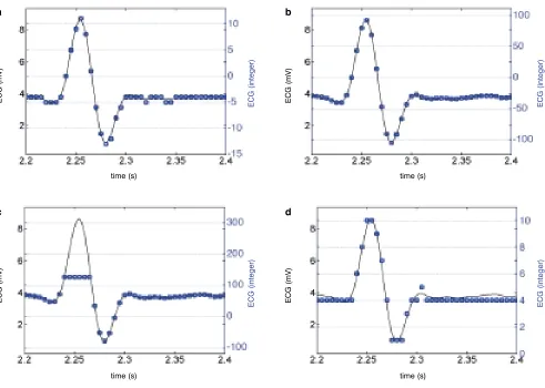
The example in fig. 5 illustrates an A/D converter that has a total of 32 distinct levels (steps), covering the range ±10 mV. If the input signal exceeds this range, the A/D converter 'saturates', i.e. gives the minimum or maximum value (-16 and +15, respectively). In fig. 6a, this A/D converter is applied to a segment of ECG signal, giving integer values between 1 and 13, corresponding to the ECG signal amplitudes between about 1 and 9 mV. The quantization of

Figure 4. A segment of an ECG signal without (left column) and with (right column) anti-alias filtering. The samples of the signal (•) obtained at 256 Hz,

before (a) and after (b) anti-alias filtering. The anti-alias filter has clearly reduced the mains-noise, and smoothed the signal. c) The amplitude spectrum of the analogue signal, with ECG activity below about 45 Hz, and mains-noise at 50, 150, 250, 350 and 450 Hz (fundamental and odd harmonics). d) After anti-alias filtering (cut-off at 45 Hz), the higher harmonics are suppressed, and noise at 50 Hz is attenuated. Below 45 Hz, the filter has little effect. e) The amplitude spectrum of the sampled signal, if no anti-alias filter is applied. The higher harmonics of the mains noise are aliased and appear at 106, 6 (buried in the ECG signal), 94, and 62 Hz, respectively. f) The amplitude spectrum with the anti-alias filter and sampling at 256 Hz. No aliasing is evident, and the spectrum of the ECG signal itself is maintained. Note that c and d show frequencies up to 500 Hz, and e and f only up to 128 Hz.

a b

time (s) time (s)

frequency (Hz) frequency (Hz)

frequency (Hz) frequency (Hz)

ECG ECG

amplitude amplitude

amplitude amplitude

c d

the signal is clearly evident. In fig. 6b, a higher-resolution A/D converter is applied, and the quantization is almost imperceptible, and would be quite adequate for most signal processing tasks. Thus careful selection of the ‘amplitude resolution’ of the A/D converter is vital in order to ensure high quality digital signals. Any signal detail lost due to quantization cannot (normally) be recovered; very poorly quantized data may have to be discarded.

The integer output values of the A/D can be converter back to the desired units (mV in fig. 6), by applying the appropriate calibration. The final calibrated signal however still consists of a series of discreet amplitude levels.

The resolution of the A/D converter is determined by the ‘number of bits’, and the number of different amplitude

levels = 2bits_{. Thus the converter in fig. 5 and 6a used 5 bits}

giving 32 distinct levels, and the 8-bit converter in fig. 6b, 256 levels. A higher number of bits (typically 10, 12 or 16 are used) would lead to even smaller quantization errors.

Increasing the number of bits is not the only means of reducing the approximation (or error) due to quantization. The step-size of the A/D converter (the amplitude or vertical resolution) depends both on the number of bits, and the range of the converter: resolution=range/(levels-1). For the example above, with a range of 20 mV (± 10 mV) and 5 bits,

the resolution=20/(25_{-1)=0.645mV, and with 8 bits,}

0.078mV. The resolution could be improved by reducing the range. Since the signal in fig. 6 only occupies the range of approximately 1 – 9 mV (known as the ‘dynamic range’ of the signal), we could use a range of say 0 – 10 mV for the A/D converter. The results are shown in fig. 7a, again using the 5 bit converter, where clear improvement compared to fig. 6a can be observed. Note that now the integer output of the converter nearly covers the full range from –16 to 15. The equivalent can be noted for the 8-bit converter (fig. 7b). If the range of the converter is chosen too small (e.g. 0 – 5 mV in fig. 7c), the signal is clipped, as the A/D converter cannot exceed its maximum (127 for the 8-bit converter). If a very large range is chosen (-100 to 100 mV in fig. 7d), resolution again becomes very poor, and even the 8-bit A/D converter is not adequate. A good match between the dynamic ranges of the signal and the A/D converter provides for the smallest possible quantization error.

In practice, the range of the A/D converter is often fixed (or can only be adjusted according to very limited options, e.g. ±1, ±5, ± 10, 0 – 1, 0 – 5, 0 – 10 V). The gain and offset of a signal pre-amplifier is then used to adjust the signal to the range of the A/D converter (rather than adjusting the range of the converter to the signal).

How important a given quantization error is depends on the signal: a quantization error of 0.078mV is quite important in a signal that has a range of say ±1 mV, but much less so in a signal covering a range of ±5V. Furthermore, reducing the quantization error provides little benefit, if the signal is already very noisy due to other sources (e.g. mains interference or poor quality electronics). Since the quantization error is relatively easy to control (e.g. by

Figure 6. An analogue (solid line – left-hand vertical scale) and digitized (• – right hand vertical scale) ECG signal, sampled at 200 Hz using a) 5 and b) 8

bits, and a range of ± 10 mV (see fig. 5). Note that the A/D converter output is integer-valued, and that the scales are different in a and b. Due to the low number of quantization levels in a), the digital signal shows very large steps of about 0.6 mV. With a 8 bits (b), the amplitude resolution of the A/D converter is improved (step-size of 0.08 mV), and most detail is preserved.

Figure 5. Illustration of quantization: the continuous-amplitude (analogue)

samples (x-axis) are converted to discrete values (y-axis), by rounding, or truncation. Above and below the ‘range’ of the A/D converter (±10 mV), the output is saturated. In this example, the converter cannot give a value smaller than –16 or larger than +15 (integer output).

Output (integer)

Input (mV)

time (s) time (s)

ECG (mV)

ECG (integer)

a

ECG (mV)

ECG (integer)

employing a better A/D converter with finer amplitude resolution), quantization errors should normally be small compared to other (more difficult to control) sources of noise.

An A/D converter with a high number of bits will provide lower ‘quantization noise’, and may provide acceptable results even if the dynamic range of the signal and A/D converter have not been well matched. However, these converters are more expensive, and a higher number of bits may also increase the size of files in which the data is stored: an 8-bit A/D converter requires only one byte per

sample, but 2 bytes are required for a 16-bit converter3_.

Summary and Discussion

In the above we have considered the most important steps and choices in converting signals from analogue to digital form. In fig. 8 we show further examples to aid discussion and review.

The respiratory flow signal (fig. 8a) was found (by inspecting the spectrum) to have a maximal frequency content of about

20 Hz, and was sampled at 200 Hz. This sampling rate is rather higher than strictly required, leading to rather larger files than necessary. One consideration here, however, was that a number of signals were acquired simultaneously, and it is then easiest to sample all channels at the same rate, corresponding to the maximum sampling rate required.

The digitized EMG (electromyogram) signal (fig. 8b) shows amplitudes that are hard-limited at ±40. This is clearly not ‘physiological’, and is characteristic of clipping which arises when the signal exceeds the range of the A/D converter (or the amplifier). In other applications, clipping may only be observed at either the peaks or the troughs of the signal, or it may be asymmetrical, occurring at different absolute values for minima and maxima.

The blood-flow signal (fig. 8c) varies in discrete steps in amplitude, showing plateaus between steps. This is typical for signals that have been acquired with an inadequate amplitude resolution. It should be noted that these signals have been plotted, as is usual, by drawing straight lines between their samples, which enhances the stepped appearance of the data. In order to obtain a better quality

Figure 7. The analogue signal (solid line – left axis) and the sampled version (• – right axis) sampled at 200 Hz. a) 5-bit A/D converter with an amplitude range of 0-10 mV; b) 8 bit A/D converter, 0 – 10 mV; c) 8 bit A/D converter, 0 – 5 mV; d) 8-bit A/D converter, ±100 mV. Note the saturation at 5mV (integer output of 127) in c, and the poor amplitude resolution in a and d.

3_{Usually 10 or 12 bit converters also use 2 bytes of file-storage for every sample.}

time (s)

ECG (mV) _{ECG (integer)}

a

time (s)

ECG (mV) _{ECG (integer)}

b

time (s)

ECG (mV)

ECG (integer)

c

time (s)

ECG (mV)

ECG (integer)

signal, either an A/D converter with a higher number of bits should be used, or the gain of the pre-amplifier should be reduced.

The ECG signal (fig. 8d) has been sampled at 60 Hz. This is rather low (and probably too low according to the sampling theorem – though we do not know the characteristics of the anti-alias filter used in acquisition, and thus cannot be certain). Due to the low sampling rate, the samples do not

always coincide with the peaks of the ECG, and thus the peak-values appear to vary greatly between beats – much more than expected in a normal ECG. If the ECG signal had been adequately sampled, the analogue ECG signal (or a digital version sampled at an arbitrarily high frequency) could be reconstructed from the samples, to show the more constant amplitudes of the original ECG. If aliasing has occurred, then accurate calculation of intermediate sample values would of course not be possible.

Figure 8. Examples of digitized signals. a) A respiratory flow signal, sampled adequately at 200 Hz. b) An EMG signal, showing clear evidence of clipping

(saturation) at about ±40 (arbitrary units). c) A blood flow signal (from transcranial Doppler ultrasound), that shows well-defined amplitude steps, due to poor quantization. d) An ECG signal sampled at 60 Hz. Due to the low sampling rate, the peak-values appear to fluctuate strongly between beats. e) Blood pressure sampled at 40 Hz, showing an ectopic beat. f) The heart-rate, derived from the blood-pressure signal. The beat-interval varies in discrete steps corresponding to the interval between samples (0.025 ms). Note that the signals displayed here are not calibrated in terms of their amplitude, and that straight lines have been drawn between samples.

time (s) time (s)

time (s) time (s)

time (s) time (s)

Respiratory flow

Blood flow

Blood pressure

EMG

ECG

Beat

-intervals (s)

a b

c d

I consider myself an engineer – and have a certificate to prove it. I am proud to be an engineer. I do not see myself as a scientist. For me, engineering is not just an applied science in the same way that medicine isn’t either. I will try to explain.

When I was only 6, with my grandmother as baby sitter, and to my parents’ great horror when they returned, I successfully repaired a household mains fuse – the type with real wire you had to poke through a hole and fasten each end. I went on to make models of all sorts, pull to bits and sometimes repair all nature of mechanisms, electrical and mechanical and in my early teens made radio sets – with valves, high voltages etc. receiving a few nasty shocks and burns in the process. Heaven was a transistor radio kit – just two transistors, each costing 15 shillings (75p), a fortune in those days (1958) with pocket money of two shilling per week. I seemed to have a fascination about and an instinct for how things were made and worked. Naturally for those days I wanted to be an engine driver and my father

occasionally arranged for me to ride on the footplate of real steam locomotives, then still in regular service – what excitement.

Both my grandfathers were engineers. One a chemical engineer and ‘soft drinks’ entrepreneur, the other an ex-army engineer who built and raced his own cars (I still have his gold medals and cups). Is engineering genetic, much like art and music? I don’t know but having taught electronics for a long time, it is clear that some students ‘get the hang of it’ and some don’t. I am saddened though by the seeming decline of interest in ‘engineering’ hobbies amongst young people today. I have not been able to pass it on to my children. Being a whiz kid at computer games is not quite the same thing.

But to get back to ‘engineering’. Wind the clock back a few thousand years. There was no shortage of engineering achievements, many are still with us today. The techniques

What is Engineering?

Mike Bolton

Chair - IPEM Engineering Group Board

The blood pressure signal (fig. 8e), was low-pass filtered at 12 Hz, and sampled at 40 Hz, and thus adequately according to the sampling theorem. The maximum increase in blood pressure was then used as a marker to measure the time interval between beats, in order to determine the heart rate. The results are shown in fig. 8f. Since the beat-interval was determined from the number of samples between each increase, and the time between beats varies in discrete steps of 0.025 s (considering the sampling rate of 40 Hz), the beat-interval varies in rather large discrete steps. Clearly the beat-interval signal is of poor quality, and a higher sampling rate for the blood pressure signal would have lead to better results, showing smoother variations. While the sampled signal contains all the information in the original analogue data (since the sampling theorem was obeyed), precise measurement of heart-rate should be possible. However, our simple detection algorithm did not exploit the data adequately. This illustrates the important point that strict adherence to the minimum requirements of the sampling theorem does not guarantee good results. However, adequately sampled signals do allow data to be reconstructed at an arbitrary (higher) sampling rate, by using the appropriate interpolation methods. If the sampling theorem was not obeyed, such reconstruction is not

possible4_.

In many applications, particularly in biomedicine, you may only get one chance to collect the signals. It is therefore vital that signal acquisition is adequately prepared and planned. We hope this tutorial will have clarified the underlying

principles, and allow well-informed choices to be made5_.

References

[1] D. M. Simpson and A. De Stefano; ‘A Tutorial Review of the Fourier Transform’; Scope, Vol.13, Nr.1, pp. 28-33, March 2004 [2] M. Merri, D.C. Farden, J.G. Mottley, E.L. Titlebaum; ‘Sampling frequency of the electrocardiogram for spectral analysis of the heart rate variability’; IEEE Trans Biomed Eng. Vol. 37(1) pp. 99-106. January 1990;

[3] A. V. Oppenheim and R. W. Schafer; ‘Discrete Time Signal Processing’; Prentice Hall, 1989

[4] J. Proakis and D. Manolakis; ‘Digital Signal Processing’; Macmillan, New York, 1988

[5] P.S.R. Diniz, E.A.B. da Silva, S.L. Netto; ‘Digital Signal Processing System Analysis and Design’; Press Syndicate of the University of Cambridge 2002

[6] J. Jerri; ‘The Shannon sampling theorem—its various extensions and applications: A tutorial review’; Proceedings IEEE, Vol. 11, pp. 1565–1596, 1977

4_{Detailed discussion and analysis of sampling requirements for determining heart-rate from the ECG may be found in} [2]_.

5_{Further details on the theory underlying sampling may be found in standard text books, such as} [3-5]_{. Extensions of the sampling}