1
CFD assessment of multiple energy piles for ground source heat pump in heating mode
1
Yuanlong Cui
a, b, Jie Zhu
a, 2
a
Department of Architecture and Built Environment, The University of Nottingham, Nottingham
3
NG7 2RD, United Kingdom
4
b
UK Greenergy Pathways Ltd, Queens Road, Nottinghamshire, NG9 2JW, United Kingdom
5
6
ABSTRACT
7
A three-dimensional (3D) computational fluid dynamics (CFD) model of ground source heat pump (GSHP) with multiple energy piles
8
(EPs) is developed to investigate the system heating performances under continuous and intermittent operating conditions, the system
9
thermal energy outputs and coefficients of performance (COPs) are evaluated. The 3D model is meshed based on the hybrid grids with
10
tetrahedron, hexahedron unstructured and structured types, and the k-ε equations to describe the turbulence phenomena within U-tube
11
are resolved by using computational fluid dynamics (CFD) software. A good agreement with less than 12% difference between the CFD
12
model and experimental results is achieved. 10 h active and 14 h idle mode is adopted as the intermittent operating condition in this
13
study. Based on the 3D model simulation data, it is found that the average monthly COPs of the intermittent operation are 3.63, 3.58,
14
3.45, 3.21, 3.25 and 3.34 from November to April respectively, which are corresponding to 9.3%, 9.5%, 7.1%, 5.9%, 4.8% and 3.1%
15
increases relative to those of the continuous operation. Furthermore, the soil temperature under the intermittent operating condition is
16
higher than that of the continuous operation. To sum up, the intermittent operation not only contributes to the soil temperature recovery
17
but also improves the system performance, which is very favourable for the long-term operation.
18
Keywords: Energy piles, Ground heat exchangers, CFD model, Continuous operation, Intermittent operation.
19
20
21
1 Introduction
22
Energy pile (EP) can be utilized for building structural support and ground heat exchanger (GHE) for ground source heat pump (GSHP),
23
which is one of the most promising renewable energy technologies due to its low cost and high efficiency [1,2]. Normally, a GSHP
24
consists of three fundamental components: a GHE, a heat pump unit and an air duct network. Different GHE configurations involving
25
single-, double-, triple U-tube, W-shaped tube, coaxial tube or helical-shaped tube and EPs are presented in Fig.1. Ground heat transfer
26
surrounding the GHE is a key issue for the system design and performance evaluation. In order to clarify the influences of different
27
parameters on the ground heat transfer, many experimental investigations are carried out with high costs. As a result, various
two-28
2
dimensional (2D) and three-dimensional (3D) numerical approaches or commercial software packages, such as Fluent or Comsol
1
Multiphysics, are adopted recently [5, 6].
2
3
Fig. 1. The diagram of GHEs and EP [3, 4].
4
Bhutta et al. [7] reviewed CFD application in heat exchanger design, and showed that CFD technique is a good tool for predicting the
5
performances of a wide variety of heat exchangers. Li and Zheng [8] developed a 3D unstructured finite-volume numerical model based
6
on the Delaunay triangulation approach to mesh a GHE field, and found that transient analysis depends upon a short time step (one hour
7
or less). Gustafsson et al. [9] proposed two different 3D steady-state GHE models in Scandinavia using CFD software, and discovered
8
that the induced natural convective heat flow significantly reduces thermal resistance within a borehole heat exchanger (BHE).
Koohi-9
Fayegh and Rosen [10] presented a 2D transient CFD model based on finite volume method (FVM) to investigate thermal interaction
10
of the BHEs, and indicated that the distance between two BHEs, the heat flux from the BHE wall and the system operation time affect
11
the thermal interaction. Khalajzadeha et al. [11] described a 3D CFD simulation model based on the second-order response surface
12
method with the central composite design approach, and discovered that the response variables are strongly affected by the
13
dimensionless inlet fluid temperature and pipe diameter. Bouhacinaa et al. [12] carried out a 3D computational study on the turbulent
14
flow within a vertical GHE implemented by Fluent software, and displayed that the temperature at 2.5 m of depth is greater than that at
15
4.5 m by 1 °C. Li [13] developed a 3D unstructured finite volume cumulative constant heat flux model to predict the temperature
16
response factors on a short-term basis (one hour or less). Gashti et al. [14] proposed a 3D numerical heat transfer model based on finite
17
element method (FEM) to assess the performance of steel pile foundation by Comsol Multiphysics package, and illustrated that
18
temperature difference between the pile wall and inlet fluid is around 25–33%, and there is a big temperature fluctuation near the tube
19
curve. Rees and He [15] used a 3D multi-block mesh to represent BHE components for studying the fluid flow phenomena, and
20
3
is very high. Bouhacina et al. [16] investigated GHE thermal and dynamic properties using Fluent software, and indicated that the fins
1
could increase heat extraction rate about 7% and enable a faster soil temperature recovery. Cao et al. [17] studied thermal performance
2
of a novel GHE with high thermal conductivity material by using both CFD simulation and experimental test, and discovered that steel
3
pipe has a better thermal performance in comparison to polyethylene pipe with the increasing range from 14% to 20%. Dai et al. [18]
4
established a 3D transient heat transfer CFD model for a vertical GHE by considering the effect of thermal short-circuiting between two
5
legs of a U-tube, and demonstrated that the soil temperature field is in a “narrow belt shape”. Mehrizi et al. [19] studied three EPs by
6
using Gambit 2.4.6 and Fluent, and discovered that W-shaped-all round EP has the highest heat transfer rate in comparison to
1-U-7
shaped and 1-W-shaped EPs. Bezyan et al. [20] analysed thermal performances of U-, W- and spiral-shaped tubes in a pile foundation
8
by using CFD software, and found that spiral-shaped configuration has the highest heat transfer rate and biggest inlet-outlet working
9
fluid temperature difference. Kong et al. [21] studied thermal performances of GHE with different configurations by CFD simulation,
10
and concluded that the mean heat transfer rate of a smooth U-tube is improved by 43% when the working fluid flow velocity increases
11
from 0.2 m/s to 1.2 m/s. Gashti et al. [22] simulated heating and cooling operation states of a EP system by using Comsol Multiphysics
12
software, and observed high pile temperature fluctuations in both winter and summer operating periods. Bidarmaghza et al. [23]
13
developed a 3D numerical model to evaluate the impact of surface air temperature for the long-term operation by using Comsol software,
14
and revealed that accounting for the surface air temperature fluctuation could reduce GHE length up to 11% approximately.
15
The intermittent operating mode of GSHP would strengthen ground heat transfer and improve the system performance compared with
16
continuous operation. This is because soil temperature recovers more quickly in the intermittent operating mode. Shang et al. [24, 25]
17
proposed a regression formula to predict soil temperature variation under intermittent operating condition, and concluded that the soil
18
temperature reduces more quickly and recovers more slowly when the fluid flow rate is comparatively higher and the ambient air
19
temperature is relatively lower. Zhang et al. [26] presented an analytical solution for the intermittent running procedure by using a
20
composite-medium line-source method, and found that the operating time and on-off ratio are critical for soil temperature recovery, and
21
the most efficient on-off ratio ranges from 0.33 to 0.5. Cao et al. [27] developed a GHE heat transfer model based on combination of
22
the analytical and numerical solutions to study the soil heat accumulation nearby the GHE under five different intermittent operating
23
modes. They indicated that the restoration performance is the best when the intermittent ratio is 3 because of the longest stopping time,
24
and the improvement of the heat flux arising from the intermittence becomes more obvious. Gao et al. [28] compared GSHP energy
25
efficiencies between continuous and intermittent operating modes, and discovered that the intermittent process not only improves heat
26
exchange capacity but also decreases the number of GHEs.
27
A 3D finite volume model of ground source heat pump (GSHP) with multiple EPs is developed in this study by using CFD software,
28
which is used to investigate the system thermal energy output, coefficient of performance (COP) and energy consumption. In previous
29
4
[30, 31] and thermal resistance theories [32] to analyse EP heat transfer process. Furthermore, the helical and triple U-tube
1
configurations within the EP are also studied based on the CaRM improvement method for investigating transient heat transfer issues
2
and estimating the system thermal performance [33]. However in this study, the GSHP with multiple EPs is investigated to identify the
3
EP and its surrounding soil temperature distributions, and predict the GSHP heating performances under the continuous and intermittent
4
operating conditions through CFD software. This study will provide the clear temperature contours of multiple EPs for GSHP.
5
2 Numerical mechanism
6
2.1 Multiple EPs
7
In engineering practice, the EP is typically constructed by inserting one high-density polyethylene (HDPE) U-tube in an EP to serve as
8
a ground loop. This section presents multiple EPs geometrical configuration.
9
10
Fig. 2. A schematic diagram of the multiple EPs with single U-tube array layout.
11
The total pile number of is 21, which is essential for the foundation requirement of a dwelling. However, only the perimeter 16 piles
12
are utilized for heat exchange with soil. Each concrete pile has a diameter of 0.3 m and a depth of 10 m, the inserted HDPE U-tube has
13
an exterior diameter of 0.032 m with wall thickness of 0.0029 m and the EP shank space is 0.06 m [34, 35]. A schematic diagram of the
14
multiple EPs is presented in Fig. 2.
15
2.2 Building heating energy demands and heat pump unit
16
The multiple EPs system is installed in a two-storey residential building in the UK. The building with the total floor area of 144 m2 is
17
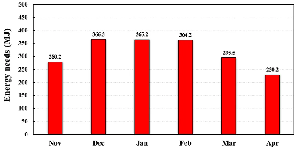
designed for one family of four persons, and its monthly heating energy requirements from November to April are shown in Fig.3 [35].
18
The maximum heating energy is 366.3 MJ in December, while the minimum is 230.2 MJ in April. The EPs are connected to a 5.9 kW
19
Greenline HT Plus heat pump [34, 35] which produces hot water at a temperature range of 35 °C to 65 °C. The main parameters of the
20
5
1
Fig. 3. Building monthly heatingenergy requirements.
2
Table 1 Nominal specification of Greenline HT Plus heat pump [34, 35].
3
Description Value
Emitted /Supplied output at 0/35°C 5.9/1.3 kW
Emitted /Supplied output at 0/50°C 5.4/1.7 kW
Minimum flow heating medium 0.14 l/s
Nominal flow heating medium 0.20 l/s
Superheat 3 °C
Refrigerant R407C mass flow rate 0.02 kg/s
Evaporating temperature (dew point) -1 °C
Condensing temperature (dew point) 58.9 °C
Evaporating pressure 4.5 bar
Condensing pressure 24.7 bar
4
2.3 Mathematical modelling
5
Heat transfer in the multiple EPs system is modelled as heat conduction and convection. Heat conduction takes place in the soil, BHE
6
backfilling material (concrete) and HDPE pipe wall, and partially in the working fluid. Heat convection dominates in the working fluid
7
circulating within the pipe. In this modelling, the working fluid flow and its heat transfer are coupled within the pipe. The coupled
8
procedure often refers to a thermal interaction process between the conductive heat transfer of the solid region and the convective heat
9
transfer of the fluid region. As a result, a 3D numerical model has been established and implemented using FVM based on the following
10
assumptions:
11
Physical properties of the working fluid are constant.12
A profile of velocity is uniform at the inlet.13
Heat transfers in the grout and soil regions are regarded as pure heat conduction and the effect of groundwater flow is negligible.14
The governing equations of the fluid flow and heat transfer are coupled numerically within the CFD software.15
6
Heat transfer within the solid region is regarded as pure heat conduction, and the corresponding energy conservation equation can be
1
given as:
2
V A
T
T
T
(ρcT)dV
(λ
λ
λ
) n dA
t
x
y
z
(1)3
Where, ρ is the density (kg/m3); c is the specific heat (J/kg·K); T is the temperature (K); t is the time (s); λ is the thermal conductivity
4
(W/m·K); V is the control volume (m3);
n
dA is the component of temperature in the direction of the vector
n
normal to surface element
5
dA.
6
The fluid energy equation to illustrate the convective-conductive heat transfer is given as [36]:
7
φ
CV CV CV CV
(ρφ)
dV div(ρφu)dV (Γ gradφ)dV S dV
t
(2)8
Where, (ρφ)
t
is the rate of change term;div (ρφu) is the convective term; Γ gradφ isthe diffusive term; Sφ is the source term.
9
The transient mathematical model is applied in 3D Cartesian coordinate system by using the k-ε turbulence model, thus the k and ε
10
conveyance equations of the standard k-ε turbulence model are obtained as:
11
t
t k k k
μ (ρ k)
div(ρ k v) div[ gradk] 2μ S S ρε
t σ v
(3)
12
2 t1ε t ε ε 2ε ε
μ
(ρε) ε ε
div(ρεv) div[ grad ε] C 2μ S S C ρ
t σ k k
v
(4)
13
Where, k is the turbulent kinetic energy per unit mass (J/kg); ε is the rate of dissipation of turbulent kinetic energy per unit mass (m2/s3);
14
Sk, Sε are the source terms; σk and σε are the Prandtl numbers of k and ε; μt is the eddy viscosity (m2/s); v is the fluid velocity vector;
15
Cμ, σɛ, σk, C1ɛ and C2ɛ are the empirical constants shown in Table 2 [36].
16
Table 2 Turbulent constants in the governing equations.
17
Cμ C1ε C2ε σk σε
0.09 1.44 1.92 1.00 1.30
18
Integration of Eq. (1) over the control volume and a time interval from t to (t+Δt) gives
19
t Δt t Δt
t CV t CV
1 T div[grad(T)]dVdt dVdt α t
(5)20
Using a fully implicit formulation, the left side of the volume integral of the temporal derivative can be written as
21
t Δt 0 P P CV t T[ ρc dt]dV ρc(T T )ΔV t
7
Where, P P0
T 1
(T T ) t Δt
has been discretised by a first-order (backward) differencing scheme, in which T is the value of T at time t P0
1
and TP is the value at time (t+Δt), Δt is the time step, and ΔV=dxdydz.
2
t Δt
0
T p p p
t
I T dt [ξT (1 ξ)T ]Δt
(7)
3
The fully implicit discretisation method is applied to this model, thereby the value of ξ is equal to 1. Owing to the transient term, the
4
time is subdivided into 4200 time steps of 3600 s which equals a time period of 180 days.
5
2.3.2 Boundary and initial conditions
6
To solve the above governing equations, appropriate boundary and initial conditions must be provided. The detailed boundary and initial
7
conditions are established as follows:
8
At z = 0, the inlet pipe temperature is equal to the fluid temperature: Tinlet (0, t) = Tfluid (t) = 1.2 °C.
9
The boundary condition at the outlet is regarded as zero gradient for all variables expect pressure.
10
The soil top surface is solid with a constant temperature of 10.4 °C which is the outside air temperature.
11
The distant and bottom surfaces are set as no-slip solid wall with a constant temperature of 15.5 °C which is the annual average
12
soil temperature.
13
The working fluid flow rate is 0.5 m3/s.
14
The main thermal physical properties of the materials are presented in Table 3.
15
Table 3 Summary of the primary input parameters utilized in the numerical models.
16
Fluid (mixture of glycol and water)
Density 1035 kg/m3
Kinematic viscosity 4.94x10⁻⁶ m2/s
Heat capacity 3795 J/(kg ·K)
Thermal conductivity 0.58 W/(m·K)
Pipe(High density polyethylene)
Density 950 kg/m3
Heat capacity 2300 J/(kg ·K)
Thermal conductivity 0.45 W/(m ·K)
Filling (Grout)
Density 1860 kg/m3
Heat capacity 840 J/(kg ·K)
Thermal conductivity 2 W/(m ·K)
Soil
Depth Thermal conductivity Density
Mixed Gravel and coarse sand 0 m to 2.22 m 1.30 W/(m·K) 2277 kg/m3
Sand gravel 2.22 m to 3.3m 1.15 W/(m·K) 2094 kg/m3
Gravelly Clay 3.3m to 5.5 m 1.68 W/(m·K) 2223 kg/m3
Gravelly Clay 5.5m to 10 m 1.75 W/(m·K) 2392 kg/m3
8
1
2.4 COP of heat pump
2
A vapour-compression heat pump model is used in this study and its parametric model reflecting the effect of compressor rotation speed
3
is adopted [37].
4
1 r,cond n r c r,suc v
r,evap P
m V ωρ [1 C (1 ) ]
P
(8)
5
n 1 r,evap r,cond n comp r,dis r,suc
r,suc r,evap
P P
n
Δξ ξ ξ [( ) 1]
n 1 ρ P
(9)
6
r comp el comp m Δξ Q η (10)
7
Where, mr is the refrigerant mass flow rate (kg/s); Vc is the compressor swept volume (m3); ω is the compressor rotational speed (rev/s);
8
ρr,suc is the compressor suction refrigerant density (kg/m3); Cv is the compressor volumetric coefficient, P is the pressure (kPa); ξ is the
9
specific enthalpy (kJ/kg), n is the polytropic compression coefficient; ηcomp is the compressor mechanical efficiency; Δξ is the specific
10
enthalpy change (kJ/kg); Qel is the electrical energy consumption (kW).
11
The COP of heat pump is defined as:
12
el heating Q COP Q (11)
13
Where Qheating is the heating capacities (kW).
14
2.5 Solution scheme
15
The geometrical model and meshing are established with a 3D domain using Gambit 2.4.6 software. Mass, momentum and energy
16
conservations of the working fluid, pipe, pile and soil are implemented via Fluent 6.3.26. The standard k-ε equations with the normal
17
wall function are selected for the working fluid and pipe. Regarding the working fluid within the pipe, a turbulent flow is considered in
18
this study. The turbulence kinetic energy (k) and dissipation rate (ε) are obtained by using numerical calculation based on the standard
19
k-ε model in 3D Cartesian coordinate system. By applying SIMPLEC algorithm, pressure–velocity coupling in the flow region is
20
acquired. The second-order upwind differencing scheme using multidimensional linear reconstruction is adopted to solve Navier-Stokes
21
equations. Furthermore, convergence is deemed to be reached when the scaled residuals are less than 10−6 for energy, 10−5 for velocity
22
and continuity and 10−3 for k and ε equations.
23
2.6 Mesh analysis
24
The mesh quality affects the accuracy of numerical simulation result. Sparse meshes make the computation fast, but sacrificing the
25
accuracy. Conversely, dense meshes generate the accurate simulation results, but requiring the long computational time. In order to save
26
9
tetrahedron, hexahedron unstructured and structured types. Figs. 4 and 5 describe the detailed meshes regarding the single and multiple
1
EPs models, respectively. Fig. 4 (a) describes the half EP involving the working fluid, pipe and pile domains, and the meshes are
2
quadrilateral with unstructured type. Fig. 4 (b) and Fig. 4 (c) present the meshes in the pipe region, meanwhile, Fig. 4 (d) displays a
3
local magnification of the meshes in U-tube bending part with triangular unstructured type. Approximately 230,000 tetrahedral elements
4
are made for single EP model. Fig. 5 (a) gives the total meshes including the soil, pile, pipe and working fluid domains, which are
5
established to complete grid independence imitation for 3D multiple EPs. More meshes are added in the soil domain nearby the EP and
6
pile domain nearby the U-tube. Thermalcapacities of these cells are modified, and the fluid mass in the whole pipe is taken into account.
7
Fig. 5 (b) shows the top surface meshes which are unstructured type. The total number of cells, faces and nodes are 540,976, 11,724,100
8
and 1,088,449, respectively.
9
10
Fig. 4. Schematic diagram of the single EP model and meshes in Gambit: (a) 3D single EP model meshes; (b) meshes for the horizontal
11
cross-section of half grout domain; (c) meshes for the horizontal cross-section of half working fluid and pipe domain; (d) meshes for
12
10
1
Fig. 5. Schematic diagram of the multiple EPs model and meshes in Gambit: (a) 3D multiple EPs model meshes; (b) top surface view
2
of the meshes.
3
3. Validation
4
In order to verify the proposed 3D model, the CFD simulation results are validated by experimental data [34], the errors are obtained
5
by Eq. (12). The experimental data gained from the facility near Birmingham, UK, are utilized in this study, the effects of main EP
6
parameters on the system performance are also analyzed.
7
numerica l exp eriment numerical
T T
Error
T
(12)
8
3.1 Pile temperatures
9
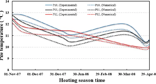
The pile temperatures at a depth of 5 m are shown in Fig. 6, the highest pile temperature is obtained from pile 10 (referring to Fig. 2).
10
The pile temperatures obtained from the simulation have the similar variation patterns as the experimental data, the maximum pile
11
temperature differences between the simulation and experimental results are 4.24%, 5.85% and 4.36% for piles 10, 11 and 12
12
respectively, as indicated in Table 4, the maximum errors occur at the initial operation time for piles 11 and 12 while it happens at the
13
middle of the operation time for pile 10. The mean temperature errors are 3.4%, 2.9% and 2.6% for piles 10, 11 and 12 respectively,
14
these data verify the developed model.
15
11
1
Fig.6. Pile temperatures at depth of 5m.
2
Table 4 Relative errors of pile temperatures.
3
Pile 10
Date CFD model results (°C) Test results (°C) Errors (%)
01/Nov/2007 18/Nov/2007 05/Jan/2008 20/Jan/2008 26/Mar/2008 23/Apr/2008 29/Apr/2008 12.45 12.26 11.11 10.80 11.55 10.12 10.24 12.88 12.74 11.41 11.08 12.04 10.45 10.65 3.45 3.92 2.70 2.59 4.24 3.26 4.00 Pile 11
Date CFD model results (°C) Test results (°C) Errors (%)
01/Nov/2007 18/Nov/2007 05/Jan/2008 20/Jan/2008 26/Mar/2008 23/Apr/2008 29/Apr/2008 12.35 11.45 10.25 10.13 11.10 10.30 10.50 12.78 12.31 10.85 10.45 11.40 10.43 10.61 3.48 5.24 5.85 3.16 2.70 1.26 1.05 Pile 12
Date CFD model results (°C) Test results (°C) Errors (%)
01/Nov/2007 18/Nov/2007 05/Jan/2008 20/Jan/2008 26/Mar/2008 23/Apr/2008 29/Apr/2008 12.12 11.25 11.01 10.98 10.15 9.78 9.92 12.51 11.74 11.44 11.38 10.26 9.96 10.06 3.22 4.36 3.91 3.64 1.08 1.84 1.41
4
3.2 Soil temperatures
5
The soil is typically stratified with different materials including sand, clay, rock and so on. The soil temperatures at the location E
6
(referring to Fig. 2) are shown in Fig. 7 in which the simulation results show similar variation trends as the experimental data at 5 m
7
12
maximum soil temperature differences between the experimental and simulation results at 5 m and 10 m depths are 12.02% and 3.92%
1
respectively, and these happen on 13th February 2008 and 25th November 2007, correspondingly, the mean soil temperature errors at 5
2
m and 10 m depths are 8.75% and 2.69%, respectively.
3
4
Fig. 7. Soil temperatures at location E.
5
These deviations could be due to the simplified assumptions in the CFD numerical model, for example, the influence of groundwater is
6
not considered in the numerical model. The errors of the soil temperature are summarized in Table 5, it can be seen that the maximum
7
error is 11.90% and the average error is approximately 10%, therefore the CFD model is effectively supported by the experimental data.
8
Table 5 Relative errors of soil temperatures.
9
Location E at 5 m soil depth
Date CFD model results (°C) Test results (°C) Errors (%)
01/Nov/2007 25/Nov/2007 15/Dec/2007 14/Jan/2008 13/Feb/2008 08/Apr/2008 29/Apr/2008 13.14 11.76 10.76 9.49 8.32 7.07 7.26 14.10 12.72 11.72 10.45 9.31 7.61 7.82 7.32 8.18 8.94 10.14 11.90 7.61 7.76
Location E at 10 m soil depth
Date CFD model results (°C) Test results (°C) Errors (%)
01/Nov/2007 25/Nov/2007 15/Dec/2007 14/Jan/2008 13/Feb/2008 08/Apr/2008 29/Apr/2008 12.10 11.74 11.83 11.87 11.89 11.83 11.77 12.56 12.20 12.18 12.17 12.16 12.08 12.02 3.80 3.92 2.96 2.53 2.27 2.11 2.11
10
4. Results and discussion
11
13
Temperature distributions of the working fluid, pile and soil domains under the continuous operating condition are presented in Figs. 8
1
to 11. Heat transfers among the working fluid, pile, and soil are not only along the axial direction of the EP but also along its radial
2
direction. The depth-diameter ratio of the EP is quite big and two branches of the U-tube are very close, these lead to the large
3
temperature variation in the radial direction.
4
4.1.1 Fluid temperatures
5
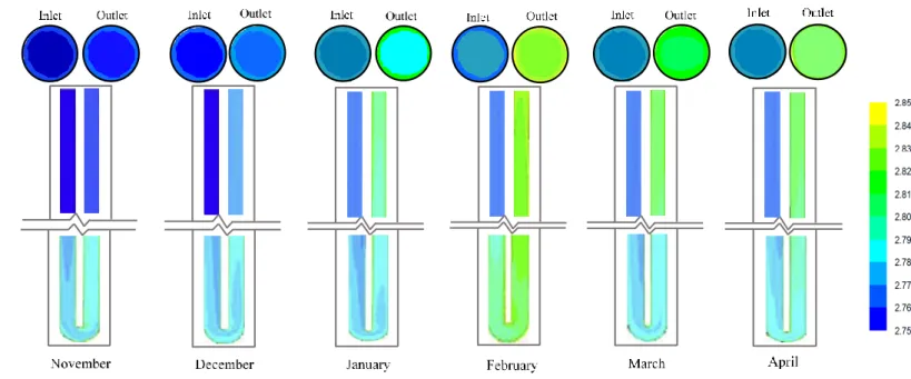
Fig. 8 shows the schematic contours of the working fluid temperature from November to April. The temperature scale is chosen to be
6
between 275 K (2 °C) to 285 K (12 °C). The fluid temperature gradually increases along the flow direction, and its variation is more
7
intensive within the outlet branch of the U-tube compared with that within the inlet branch. It can be seen that the fluid temperature is
8
not distributed homogeneously. The contours of the static temperature display that the outlet fluid temperature increases from 276.80
9
K (3.80 °C) at the end of November to 281.75 K (8.25 °C) at the end of February, then decreases to 278.95 K (5.45 °C) at the end of
10
April.
11
12
Fig. 8. Contours of fluid temperature distributions.
13
4.1.2 Pile temperatures
14
Fig. 9 presents the pile temperature variations in the axial and radial directions, Fig. 9 (b) depicts the sectional axonometric diagram of
15
single EP while Fig. 9 (c) gives 3D EP temperature distributions at different layers. Fig. 9 (d) and Fig. 9 (e) illustrate the temperature
16
distributions of a single EP in the axial and radial directions from November to April. The temperature scale ranges from 275 K (2 °C)
17
to 289 K (16 °C). It is found that the pile temperature dramatically reduces from 285.45 K (12.45 °C) in November to 283.00 K (10.00 °C)
18
14
1
Fig. 9. Pile temperature distributions: (a) 3D model; (b) half an EP; (c) single EP at different depths; (d) top view of single EP; (e) single
2
EP in the axial direction.
3
4.1.3 Soil temperatures
4
The soil temperature distributions from November to April are given in Figs. 10 and 11. At the initial stage, more heat is extracted from
5
the soilowing to the low inlet fluid temperature. As can be seen from Fig. 10, the largest deviation of the isotherm in the ground appears
6
in April. This is because the soil temperature decreases with operation time. 3D cutaway views regarding soil temperature distribution
7
are shown in Fig. 11 in detail, it can be seen clearly that the soil temperature nearby the EP decreases dramatically from 288.5 K (15.5 °C)
8
15
1
Fig. 10. 3D soil temperature distributions.
2
3
Fig. 11. Soil temperature distributions in the axial direction.
4
4.1.4 System performances
5
The system daily thermal energy outputs are given in Fig. 12. It is found that the daily thermal energy outputs are lower in November
6
and April than those in the middle period (from December to March). Notably, the system maximum daily thermal energy output is
7
16
1
Fig. 12. Daily thermal energy outputs.
2
3
Fig. 13. Daily power consumptions and COPs.
4
Fig. 13 depicts the daily variations of the system COP and power consumption. It can be seen that the power consumption variation
5
trend is similar to the heating load’s referring to Fig. 3. The maximum daily power consumption reaches approximately 398.6 MJ on
6
17th December 2007, the mean being 218.6 MJ, while the minimum is about 24.2 MJ on 21st April 2008. The maximum COP is
7
approximately 3.39, the average being 3.21, while the minimum reaches around 2.91. Some previous studies present the similar COP
8
variations. For instance, 16 GHEs with an 80 kW nominal power of heat pump unit are investigated in Padua, Italy [38], and discovered
9
that the COP varies from 3.7 to 4.5 in heating season. Furthermore, 9 GHEs with a 23.96 kW heating capacity heat pump are studied
10
for an office building in Hong Kong [39], and found that COP range of 3.85 to 4.20 is obtained for this case study. 49 EPs with 171.2
11
kW nominal capacity of heat pump are simulated for one storey commercial hall building in Finland, and indicated that the average
12
17
Fig. 14 shows the building heating energy demands and the system thermal energy outputs. The system thermal energy outputs far
1
exceed the actual building heating demands, this means that the system continuous operation leads to huge waste of energy resource.
2
Therefore, in order to avoid this problem, the system intermittent operation strategy is investigated based on the developed 3D model.
3
4
Fig. 14. Thermal energy demands and outputs.
5
4.2 Intermittent operation
6
3D numerical simulations are implemented to analyse the system performance under intermittent operating condition. Based on the data
7
in Fig. 14, the average ratio of thermal energy output to building heating load is approximately 0.45, which is equivalent to 10 hours of
8
operation time per day. Thereby, in this study, 10 h active and 14 h idle mode is set as the intermittent operating strategy for assessing
9
the system performance.
10
11
Fig. 15. Thermal energy outputs: (a) daily; (b) hourly in the first 4 days.
12
Fig. 15 (a) displays the simulation results of the daily heat pump thermal energy output for the whole heating period. As shown in this
13
figure, the variation trend of intermittent operation is similar to the continuous operation’s referring to Fig. 12. The intermittent daily
14
thermal energy outputs are lower than those under the continuous operation condition due to the short operating time. Notably, the
15
system maximum daily thermal energy output is approximately 892.3 MJ on 1st December 2007, and the minimum value is around 23.9
16
18
energy output increases after each intermittence, for example, the thermal energy output at the fourth day intermittence is 198.8 MJ
1
while it is only 162.9 MJ at the first day. This is owing to the soil temperature recovery.
2
3
Fig. 16. COPs and power consumptions: (a) daily; (b) hourly in the first 4 days.
4
Fig. 16 (a) displays the system daily mean COPs and power consumptions during the intermittent operation period. Obviously, the COP
5
variation trend of the intermittent operation is similar to the continuous operation’s referring to Fig. 13. It can be found that the maximum
6
COP is approximately 3.71, the average being 3.41, while the minimum reaches around 3.09. The intermittent COPs increase
7
approximately 6.67% compared with those under the continuous operating condition. Meanwhile, the maximum daily power
8
consumption approximately is 249.9 MJ on 1st December 2007, while the minimum value reaches 7.3 MJ on 21st April 2008. In
9
comparison to the continuous operation, the daily mean power consumption under theintermittent operating condition is lower owing
10
to the cease of the heat pump system. The detailed intermittent COP variations and power consumptions in the first 4 days are shown
11
in Fig. 16 (b). From this figure, it can be obtained that the COP variations are fluctuant. The COPs reduce from 3.83, 3.81, 3.79 and
12
3.78 at the beginning of intermittence to 3.62, 3.6, 3.59 and 3.58 at the end of intermittence from the first day to the fourth day,
13
respectively. Furthermore, the power consumption variations are also fluctuant, the maximum hourly power consumption approximately
14
reaches 45 MJ on the first day, 48.5 MJ on the second day, 52 MJ on the third day and 55.6 MJ on the fourth day. To sum up, both
15
thermal energy output and power consumption gradually increase, but the heat pump COP decreases.
16
4.3 Comparison between the continuous and intermittent operations
17
Figs. 17 to 19 show monthly thermal energy outputs, COPs and power consumptions under the continuous and intermittent operations.
18
As shown in Fig. 17, the system is capable of meeting the building heating demand under both operating conditions. As can be seen
19
from Fig. 18, the monthly power consumptions of the heat pump are 89.5 MJ, 120.1 MJ, 121.9 MJ, 123.5 MJ, 104.9 MJ and 76.1 MJ
20
from November to April under the intermittent operating condition, with corresponding power saves of approximately 43.4%, 55.9%,
21
55.6%, 55.3%, 46.9% and 44.4%, respectively, compared with those under the continuous condition. As indicated in Fig. 19, the average
22
monthly COPs of the intermittent operating condition are higher than those of the continuous operating condition. The average monthly
23
COPs of the intermittent operating condition are 3.63, 3.58, 3.45, 3.21, 3.25 and 3.34, with corresponding increases of 9.3%, 9.5%,
24
19
1
2
Fig. 17. Thermal energy demands and outputs under continuous and intermittent operations.
3
4
Fig. 18. The monthly power consumptions under continuous and intermittent operations.
5
6
Fig. 19. The mean COPs under continuous and intermittent operations.
7
Fig. 20 illustrates the location E soil temperature variations under the continuous and intermittent operating conditions at depth of 5 m.
8
20
the soil temperature recovers when the heat pump is shut down. The soil temperature recovery not only leads to the soil heat
1
accumulation but also improves the system performance, which is very favourable for the long-term operation. The proposed
2
intermittent operating strategy does not only contribute to improving the system performance, but also avoid the waste of energy
3
resources. Some previous studies [24-28] also indicate that the optimum intermittent time is a significant factor for the GSHP system.
4
Their results show that the most efficiency on-off ratio ranges from 1/3 to 1.
5
6
Fig. 20. The soil temperature variations.
7
5. Conclusions
8
A 3D finite volume model of GSHP with multiple EPs system is developed based on the CFD software in this paper. Sixteen concrete
9
piles are adopted as heat exchangers, and a 5.9 kW nominal heat pump is connected with the EPs in this study. A comparison between
10
the numerical data and experimental results shows a good agreement with less than 12% difference. The system thermal energy outputs
11
far exceed the building heating energy demands under the continuous operating condition, so an intermittent operating strategy (10 h
12
active and 14 h idle) is adopted to avoid energy waste and improve the system performance. Furthermore, the comparisons of monthly
13
thermal energy outputs, COPs and power consumptions between the continuous and intermittent operating conditions are carried out.
14
The following conclusions are drawn from this study:
15
(1) The system maximum thermal energy output is 1299.6 MJ and the minimum is 76.4 MJ under the continuous operating condition,
16
while the maximum and minimum values under the intermittent operating condition are 892.3 MJ and 23.9 MJ, respectively.
17
(2) The monthly power savings of the intermittent operating condition from November to April are 43.4%, 55.9%, 55.6%, 55.3%, 46.9%
18
and 44.4% compared with those of the continuous operating condition.
19
(3) The mean monthly COPs of the intermittent operating condition are 3.63, 3.58, 3.45, 3.21, 3.25 and 3.34 from November to April,
20
with corresponding improvements of 9.3%, 9.5%, 7.1%, 5.9%, 4.8% and 3.1% respectively, compared to the continuous operation’s
21
(3.32, 3.27, 3.22, 3.03, 3.10 and 3.24).
22
(4) The soil temperatures of the intermittent operation are higher than those of the continuous operation due to heat recovery for the
23
21
(5) This intermittent operation gives better COP and saves more energy compared with the continuous operation. The optimum
1
intermittent operation strategy is critical to improve the system performance.
2
3
References
4
[1] H. Esen, M. Inalli, Y. Esen Y, Temperature distributions in boreholes of a vertical ground-coupled heat pump system, Renewable
5
Energy 34 (2009) 2672–2679.
6
[2] G. A. Akrouch, M. Sánchez, J. L. Briaud, An experimental, analytical and numerical study on the thermal efficiency of energy piles
7
in unsaturated soils, Computers and Geotechnics 71 (2016) 207–220.
8
[3] J. Gao, X. Zhang, J. Liu, K. Li, J. Yang, Thermal performance and ground temperature of vertical pile-foundation heat exchanger:
9
a case study, Apply Thermal Engineering 28 (2008) 2295–2304.
10
[4] Y. Hamada, H. Saitoh, M. Nakamura, H. Kukbota, K. Ochifuji, Field performance of an energy pile system for space heating, Energy
11
and Buildings 39 (5) (2007) 517–524.
12
[5] A.G. Kanaris, A.A. Mouza, S.V. Paras, Flow and heat transfer prediction in a corrugated plate heat exchanger using a CFD code,
13
Chemical Engineering & Technology. 8 (2006) 923-930.
14
[6] Y. Wang, Q. Dong, M. Liu, Characteristics of fluid flow and heat transfer in shell side of heat exchangers with longitudinal flow of
15
shell side fluid with different supporting structures, Challenges of Power Engineering and Environment (2007) 474-479.
16
[7] M. Bhutta, N. Hayat, M. H. Bashir, A. R. Khan, K. N. Ahmad, S. Khan, CFD applications in various heat exchangers design: a
17
review, Applied Thermal Engineering 32 (2012) 1-12.
18
[8] Z. Li, M. Zheng, Development of a numerical model for the simulation of vertical U-tube ground heat exchangers, Applied Thermal
19
Engineering 29 (2009) 920–924.
20
[9] A. M. Gustafsson, L. Westerlund, G. Hellström, CFD-modelling of natural convection in a groundwater-filled borehole heat
21
exchanger, Applied Thermal Engineering 30 (2010) 683–691.
22
[10] S. Koohi-Fayegh, M. A. Rosen, Examination of thermal interaction of multiple vertical ground heat exchangers, Applied Energy
23
97 (2012) 962–969.
24
[11] V. Khalajzadeha, G. Heidarinejada, J. Srebric, Parameters optimization of a vertical ground heat exchanger based on response
25
surface methodology, Energy and Buildings 43 (2011) 1288–1294.
26
[12] B. Bouhacinaa, R. Saima, H. Benzenineb, H.F. Oztopc, Analysis of thermal and dynamic comportment of a geothermal vertical
U-27
tube heat exchanger, Energy and Buildings 58 (2013) 37–43.
28
22
[14] E. H. N. Gashti, V.M. Uotinen, K. Kujala, Numerical modelling of thermal regimes in steel energy pile foundations: A case study,
1
Energy and Buildings 69 (2014) 165-174.
2
[15] S. J. Rees, M. He, A three-dimensional numerical model of borehole heat exchanger heat transfers and fluid flow, Geothermics 46
3
(2013) 1–13.
4
[16] B. Bouhacina, R. Saim, H.F. Oztop, Numerical investigation of a novel tube design for the geothermal, Applied Thermal
5
Engineering 79 (2015) 153–162.
6
[17] S. Cao, X. Kong, Y. Deng, W. Zhang, L. Yang, Z. Ye, Investigation on thermal performance of steel heat exchanger for ground
7
source heat pump systems using full-scale experiments and numerical simulations, Applied Thermal Engineering 115 (2017) 91–
8
98.
9
[18] L. Dai, Y. Shang, X. Li, S. Li, Analysis on the transient heat transfer process inside and outside the borehole for a vertical U-tube
10
ground heat exchanger under short-term heat storage, Renewable Energy 87 (2016) 1121–1129.
11
[19] A. A. Mehrizi, S. Porkhial, B. Bezyan, H. Lotfizadeh, Energy pile foundation simulation for different configurations of ground
12
source heat exchanger, International Communications in Heat and Mass Transfer 70 (2016) 105–114.
13
[20] B. Bezyan, S. Porkhial, A. A. Mehrizi, 3-D simulation of heat transfer rate in geothermal pile-foundation heat exchangers with
14
spiral pipe configuration, Applied Thermal Engineering 87 (2015) 655-668.
15
[21] X. Kong, Y. Deng, L. Li, G. Gong, S. Cao, Experimental and numerical study on the thermal performance of ground source heat
16
pump with a set of designed buried pipes, Applied Thermal Engineering 114 (2017) 110–117.
17
[22] E. H. N. Gashti, V. M. Uotinen, K. Kujala, Numerical modelling of thermal regimes in steel energy pile foundations: A case study,
18
Energy and Buildings 69 (2014) 165–174.
19
[23] A. Bidarmaghza, G.A. Narsilio, I.W. Johnston, S. Colls, The importance of surface air temperature fluctuations on long-term
20
performance of vertical ground heat exchangers, Geomechanics for Energy and the Environment 6 (2016) 35–44.
21
[24] Y. Shang, M. Dong, S. Li, Intermittent experimental study of a vertical ground source heat pump system, Applied Energy 136
22
(2014) 628–635.
23
[25] Y. Shang, S. Li, H. Li, Analysis of geo-temperature recovery under intermittent operation of ground-source heat pump, Energy and
24
Buildings 43 (2011) 935-43.
25
[26] L. Zhang, Q. Zhang, M. Li, Y. Du, A new analytical model for the underground temperature profile under the intermittent operation
26
for ground-coupled heat pump systems, Energy Procedia 75 (2015) 840-846.
27
[27] X. Cao, Y. Yuan, L. Sun, B. Lei, N. Yu, Yang X, Restoration performance of vertical ground heat exchanger with various
28
23
[28] Q. Gao, M. Li, M. Yu, Experiment and simulation of temperature characteristics of intermittently-controlled ground heat exchanges,
1
Renewable Energy 35 (6) (2010) 1169–1174.
2
[29] D. Bozis, K. Papakostas, N. Kyriakis, On the evaluation of design parameters effects on the heat transfer efficiency of energy piles,
3
Energy and Buildings 43 (2011) 1020–1029.
4
[30] P. Hu, J. Zha, F. Lei, N. Zhu, T. Wu, A composite cylindrical model and its application in analysis of thermal response and
5
performance for energy pile, Energy and Buildings 84 (2014) 324–332.
6
[31] T.V. Bandos, A. Campos-Celador, M. Luis, L.M. Lopez-Gonzalez, J.M. Sala-Lizarraga, Finite cylinder-source model for energy
7
pile heat exchangers: Effects of thermal storage and vertical temperature variations, Energy 78 (2014) 639-648.
8
[32] F. Loveridge, W. Powrie, 2D thermal resistance of pile heat exchangers, Geothermics 50 (2014) 122-135.
9
[33] A. Zarrella, M.D. Carli, A. Galgaro, Thermal performance of two types of energy foundation pile: Helical pipe and triple U-tube,
10
Applied Thermal Engineering 61 (2013) 301-310.
11
[34] C. J. Wood, Investigation of Novel Ground Source Heat Pump, in: Built Environment, Vol. Doctor of Philosophy, University of
12
Nottingham, 2009.
13
[35] C. J. Wood, H. Liu, S.B. Riffat, An investigation of the heat pump performance and ground temperature of a piled foundation heat
14
exchanger system for a residential building, Energy 35 (2010) 4932-4940.
15
[36] H. K. Versteeg, W. Malalasekera, An introduction to computational fluid dynamics, the finite volume method, Pearson Prentice
16
Hall, 2007.
17
[37] H. Jin, J.D. Spitler, A parameter estimation based model of water-to-water heat pumps for use in energy calculation programs,
18
ASHRAE Transactions 108 (2002) 4493-4510.
19
[38] M.D. Carli, M. Tonon, A. Zarrella, R. Zecchin, A computational capacity resistance model (CaRM) for vertical ground-coupled
20
heat exchangers, Renewable Energy 35 (2010) 1537-1550.
21
[39] C.K. Lee, Effect of borehole short-time-step performance on long-term dynamic simulation of ground-source heat pump system,
22
Energy and Buildings 129 (2016) 238–246.
23
[40] J. Fadejev, J. Kurnitski, Geothermal energy piles and boreholes design with heat pump in a whole building simulation software,
24
Energy and Buildings 106 (2015) 23–24.
25
26
27
Nomenclature
A Area (m2)
24 Cv Volumetric coefficient of compressor
d Diameter (m)
h Heat transfer coefficient (W/(m2·K)) H Height (m)
k Turbulent kinetic energy per unit mass (J/kg) L Length (m)
mr Refrigerant mass flow rate (kg/s) n Polytropic compression coefficient P Pressure (kPa)
t Time interval (s) T Temperature (K)
Vc Swept volume of compressor (m3)
Greek Letters
α Ground thermal diffusivity (m2/day) ∆ Change/difference
λ Ground thermal conductivity (W/m·K) ρ Density (kg/m3)
ε Rate of dissipation of turbulent kinetic energy per unit mass (m2/s3)
σk, σε Prandtl numbers of k and ε μt Eddy viscosity (m2/s)
ω Rotational speed of compressor (rev/s)
ξ Specific enthalpy (kJ/kg)
Δξ Specific enthalpy change (kJ/kg)
η Efficiency (%)
Abbreviations
25 CV Control Volume
FEM Finite Element Method FVM Finite Volume Method GHE Ground Heat Exchanger GSHP Ground Source Heat Pump HDPE High Density Polyethylene HP Heat Pump
![Fig. 1. The diagram of GHEs and EP [3, 4]. 4](https://thumb-us.123doks.com/thumbv2/123dok_us/8554848.363886/2.892.181.719.174.519/fig-diagram-ghes-ep.webp)