Mantle Structures
Thesis by
Teh-Ru Alex Song
In Partial Fulfillment of the Requirements
for the Degree of
Doctor of Philosophy
1 8 9 1
C A
LI F
O
RN IA IN
S TIT U T E O F TE
C
H
N
O
L O G Y
California Institute of Technology
Pasadena, California
2006
(Submitted 6/23/2006)
c
2006
Teh-Ru Alex Song
Mantle Structures
Thesis by
Teh-Ru Alex Song
In Partial Fulfillment of the Requirements
for the Degree of
Doctor of Philosophy
1 8 9 1
C A
LI F
O
RN IA IN
S TIT U T E O F TE
C
H
N
O
L O G Y
California Institute of Technology
Pasadena, California
2006
(Submitted 6/23/2006)
Acknowledgements
Being at Caltech has been a special experience for me. I would like to first thank my
advisor, Don Helmberger. He gives me unlimited freedom to basically do whatever I
want. During my 6 years stay at Seismo Lab, Don has presented me with enthusiam
for picking apart every wiggle of the seismogram and has emphasized the significance
of looking at the data. Even during the end of my phD, Don allowed me to complete
my thesis any place I desired and I am so grateful for his kindness and consideration.
Besides, chating with him on basketball is always entertaining and fun. Thank you
Don !
During the past few years, seismo lab has given me great opportunities to work
on different topics with Mark Simons, Jeroen Tromp and Hiroo Kanamori. Every
one of them presents a unique personality and style of research. It certainly put an
imprint on how I deal with different problems. Working with them is such a wonderful
experience and thank them so much for guiding me through various difficulties. In
addition, Don Anderson Mike Gurnis and Paul Asimow all provided great ideas about
my research and thesis and gave me lots of valuable comments.
Of course, many people have given me a hand when I needed it the most. To
name a few: Chen Ji often behaves like a big brother and we always have great time
discussing various problems. Certainly, Qinya’s presence gives me a different outlook
on life and has helped me throughout the years. I thank her so much and wish her the
best. During difficult times in my phD, my landlord Helen treated me like family and
made me feel at home. Without her, it would not have been possible to complete the
thesis. Also, I am grateful for the help and company from my office mates, Evelina,
Abstract
Broadband seismic arrays have provided unprecedented data sets for seismologists to
image the slips on faults and velocity structure beneath Earth’s surface at all scales.
In particular, plate boundary zones are the most complicated regions on the surface
and full of complexities. Often that great earthquakes occur and rapid structural
changes take place.
In my thesis, one major effort is to use geophysical data and broadband seismic
data to characterize the occurrences of great earthquakes at the subduction zone
interface. Using gravity data from satellite and bathymetry model ETopo5, I
recog-nized the strong correlation between gravity, topography and the occurrences of great
earthquakes. Such a correlation gives a strong indication that lateral variations in the
occurrences of great earthquakes at a given subduction zone are strongly linked to the
fore-arc structure and topographic features such as basin and peninsulas. I also give
robust estimates of the size and rupture extent of the recent 2004 Sumatra-Andaman
giant earthquake using Earth’s normal modes.
Another part of my thesis consists of modeling waveform distortion and
interfer-ence to study lithosphere and deep upper mantle structure. Modeling multi-pathing
associated with sharp structure has become a very powerful method to delineate
structure and explain the complicated behavior shown in the data recorded by dense
arrays.
Future research will focus on linking geodynamic models and seismic analysis of
broadband waveform data as a way to further constrain the mantle structure and
Overview
0.1
Introduction
Plate tectonics has become one of the most successful theories describing the
kinemat-ics of the movement of the solid Earth. Great earthquakes occur mostly in the plate
boundary, especially at the subduction zone interface. However, the occurrences of
these great earthquakes are not uniform and vary substantially among different
sub-duction zones. Even within a given subsub-duction zone, the release of energy is not
uniform but rather shows significant lateral variations. It is not clear what controls
these spatial differences and over what time scale they form and persist.
Giant earthquakes (Mw > 9) rarely happen but generate tremendous energy.
The 2004 Sumatra-Andaman giant earthquake ruptured the Sunda Arc, generating a
huge tsunami. To accurately estimate the size of this event, I model very long period
normal modes (> 1000 sec) using a centroid and finite rupture model. This gives
robust estimate on the size of this earthquake and its rupture extent, while it can
also validate rupture models constructed using surface waves and body waves.
Seismic structures usually change very rapidly near the place where deformations
occur currently or in the past. While velocity structures near plate boundary zones
often vary rapidly, there are deformation zones within the plate interior that also
show large contrast in seismic structures. Recent dense broadband seismic networks
and PASSCAL experiments provide excellent chances to explore such complexities.
This thesis is divided into two parts. The first part focuses on the great
earth-quakes occurring at the subduction zone interfaces and contains chapter 1 and
subduction zone interfaces using gravity data and topography data. In addition, it
contains modeling of unprecedented, very-long-period normal modes data of the 2004
Sumatra-Andaman giant earthquake. The second part of the thesis focuses on the
broadband modeling of upper mantle triplications (Chapter 3, Chapter 4) and wave
diffractions along dipping lithosphere structures (Chapter 5, Chapter 6).
In Chapter 1, I present analysis of satellite gravity data and topography data of
global subduction zones and associate them with the occurrences of great earthquakes
at the subduction zone interfaces. Though the convergence velocity of the plate and
its age have been suggested to relate to the occurrence of great earthquakes at different
subduction zones, lateral variations in the occurrences of great earthquakes along a
given subduction zone suggests mechanical properties at the subduction zone interface
might change rapidly as well, due to differences in fluid content, sediment thickness,
structures in the upper plate, etc. Gravity has long been used as a proxy to study the
variation in stress in the crust and mantle. Here I correlate the gravity, topography
and the occurrences of great earthquakes and find a strong correlation between spatial
variations in gravity, topography and the occurrences of great earthquakes in the
forearc regions. I discuss the importance of such a strong correlation and its link to
geological structure at million years time scale.
In Chapter 2, I present modeling of very long period free Earth’s oscillations of the
Sumatra-Andaman giant earthquake. This giant event occurred on 24 December 2004
near northern Sumatra and ruptured northward more than 1000 km to the Andaman
Islands. Sea floor deformation caused by the displacement along the subduction
zone interface produced a tsunami that caused tremendous fatalities and damage.
However, the size and rupture extent were not clear even soon after the disaster.
Harvard CMT solution and teleseismic body wave inversion both indicated that the
earthquake centroid was near 3◦ −4◦N and the moment magnitude near Mw 9.0.
However, these results underestimated the amplitude of long period surface waves (>
500 secs) and very long period normal modes (>1000 secs). I find that the splitting
pattern of the gravest mode 0S2 singlets provided indisputable evidence that this
7.5◦N. Using coupled-mode theory, I also model the modal spectrum below 1 mHz
and constrain the finite fault model to explain very broadband seismic data in the
10-3300 secs period. Such approach is essential in studying great earthquakes.
In Chapter 3, I present direct S wave triplication data to investigate the extent of a
possible low velocity layer in the deep upper mantle beneath the northwestern United
States. In particular, I find that the secondary branch AB at the epicentral distance
of 21◦−24◦ is powerful. At these ranges, the strong AB branch is bottoming near
the depth of the 410 discontinuity and serves as a nice proxy of the existence of a low
velocity layer (or low velocity gradient) atop the 410. Such a low velocity layer atop
the 410 has major potential implications for the water content in Earth’s transition
zone. Modeling waveform data recorded at TriNet and several other PASSCAL arrays
for several events offshore Oregon and Washington, I map out the extent of such low
velocity layers. I also examine the consistency of my model with previous receiver
function results and find they are complementary to each other.
In Chapter 4, I extend the analysis in Chapter 3 from 1D models to 2D finite
difference models but focus on the dataset recorded by TriNet from events offshore
Oregon. This dataset presents clear evidence of a sharp velocity contrast in the
deep upper mantle changing from east to west. Such 3D waveform behavior can be
reproduced with a simple model consisting of a low velocity zone in the deep upper
mantle beneath northeastern California but diminishes rapidly to the northwest. Such
a sharp change in velocity above the 410 is very useful to characterize the origin of
this low velocity anomaly in the deep upper mantle.
In Chapter 5, I explore the usefulness of amplitude information and waveform
distortion in validating existing travel time tomography models. For example, we
consider waveform data recorded at La Ristra Transect across the Rio Grande Rift
in the southwestern United States from events beneath South America. Synthetics
produced by the original travel time tomographic model do not explain the waveform
distortion and amplitude variations presented in the data. We consider an amplified
tomographic model with a slab-like feature extending to about 600 km that has a much
model gives a much better fit to the amplitude variation and waveform distortions.
A simplified model constructed independently also shows a consistent result.
Incom-ing waves propagatIncom-ing through such a dippIncom-ing velocity contrast produce waveform
distortion and amplitude decay through diffraction along the boundary. Systematic
investigations show how to constrain the geometry and amplitude of such a dipping
velocity contrast, which is complementary to travel time delay measurement.
Consis-tent modeling of both P and S waveform distortion and amplitude decay are shown
later in Chapter6 with some speculations on the origin of such a dipping structure
near the edge of the Great Plains and the Rio Grande Rift.
In Chapter 6, I present results of modeling P and S waveform distortions across the
slab-like feature beneath the edge of the western Great Plains and the Rio Grande
Rift. I use the preferred amplified S model and scale it to the P model using a
scaling factor dlnV s/dlnV p. Such a simple procedure produces a consistent model
that explains the whole dataset from exactly the same source-receiver pairs. Incoming
waves sampling this dipping structure give direct constraints on its physical origin.
The modeling result gives a relatively low scaling factordlnV s/dlnV p, which suggests
Chapter 1
Abstract
We demonstrate that great earthquakes occur predominantly in regions with strongly
negative trench parallel gravity anomalies (TPGA), whereas regions with strongly
positive TPGA are relatively aseismic. These observations suggest that, over time
scales up to at least 1 My, spatial variations of seismogenic behavior within a given
subduction zone are stationary and linked to the geological structure of the fore-arc.
The correlations we observe are consistent with a model in which spatial variations in
frictional properties on the plate interface control variations in fore-arc topography,
gravity, and seismogenic behavior. (Originally published as Song and Simons, Science,
1.1
Introduction
Studies of profiles of the gravity field taken perpendicular to the strike of subduction
zones suggest that trench-normal gravity profiles are predominantly controlled by
mantle rheology, slab buoyancy, and interplate shear tractions on the plate interface
(1-8). Under the premise that spatial variations in gravity over the fore-arc serve as
a proxy for the long term state of stress on the plate interface, we investigate
trench-parallel gravity anomalies (TPGA) using global marine gravity grids (9, 10). The
large amplitude, longer wavelength trench-normal gravity variations can overwhelm
the smaller amplitude TPGA (Fig. 1.1A).
Therefore, in constructing maps of TPGA, we subtract an average regional
trench-normal gravity profile from the original free-air gravity data (11, 12, Fig. 1.1B). For
this analysis, we are only concerned with TPGA over the location of the plate
inter-face where large thrust earthquakes occur (less than 50 km). We hypothesize that the
large amplitude variations of TPGA that we observe (order of 40 mGal) correspond
to variations in shear tractions on the plate interface, which are in turn dependent on
normal tractions and the coefficient of friction, and may impact the seismogenic
char-acter of a given subduction zone. To test this hypothesis, we compare our estimates
of TPGA with co-seismic distributed slip models from selected earthquakes, as well
as with the epicenters of large earthquakes from the Harvard CMT and relocated ISC
global catalogs (13-15). We first consider the three largest earthquakes of the century:
1960 Chile (moment magnitude,Mw 9.5), 1964 Alaska (Mw 9.2) and 1952 Kamchatka
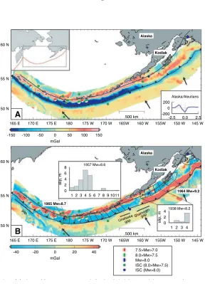
(Mw9.0). For the Alaska/Aleutians subduction zone, we find a strong visual
correla-tion between the locacorrela-tion of the principal areas experiencing large co-seismic slip in
the 1964 Alaska earthquake (Mw 9.2) (16) and negative TPGA (Fig. 1.1B). A region
of lower co-seismic slip between the two high-slip areas correlates with a region of
pos-itive TPGA (Fig. 1.1B). Regions of large co-seismic slip, as inferred from distributed
slip models of the 1938 Alaska (Mw 8.3), 1957 Aleutian (Mw 8.6), and 1965
Aleu-tian (Mw 8.7) earthquakes (17, 18), also occur predominantly in regions of negative
pressions and the locations of great earth-) is equivalent to the correlation
Along-strike variations in the position of ) relative to the trench can also be considered as a form of TPTA. For instance, models of coseismic slip from the
30)
show that the region of notable coseismic slip terminated just south of the Mejillones Pe-ninsula. It remains to be seen whether slip in the seismic gap to the north (last ruptured in 1877) will extend under the peninsula or stop just north of it. Similarly, no large coseismic slip is inferred to have occurred below Cape Muroto during the 1946 Nankai earthquake ), and during the 1960 Chilean earth-quake, coseismic slip is inferred to have de-creased substantially before reaching the pe-n (fig. ). The correlation of bathymetric highs with the absence of great earthquakes ) is equivalent to the correlation with
We find that TPGA and TPTA are positive-ly correlated in most areas, with little area in regions where TPTA and TPGA are uncorre-lated (Fig. 2B; fig. S7). This correlation is expected because gravity anomalies are intrin-sically tied to topographic variations by a given compensation mechanism. Results from
vis-7),
) suggest that spa-tial variations in the magnitude of shear trac-tions on the plate interface can modulate sur-face topography and gravity in the fore-arc. In particular, these models indicate that increasing shear tractions on the plate interface induce a decrease in vertical compressive stress, thereby depressing fore-arc topography and gravity. Consistent with these models, we interpret our observations of TPGA and TPTA as indications of variations in shear tractions on the plate
[image:17.612.180.468.62.461.2]convergence rate of the subducting plate (35) suggests that the implied increases in shear
Fig. 1.(A) Observed free-air gravity anomaly for the Alaska/Aleutian subduction zone. The average
Figure 1.1: (A) Observed free-air gravity anomaly for the Alaska/Aleutian subduction
zone. The average trench-normal gravity profile is calculated for the region shown in the inset and is shown in the sub-panel of Fig. 1.1A, with the horizontal axis being trench-normal distance in degrees and vertical axis being gravity in mGal. The color bar shows the amplitude of the free-air gravity anomaly. (B) Estimated TPGA for the Alaska-Aleutian subduction zone. The color bar shows the amplitude of TPGA. For the 1938 and 1957 events (17, 18), we indicate their respective slip distributions in the inset panels and the fault parameterization is indicated on the TPGA map. Areas with large co-seismic slip during 1964 Alaska and 1965 Aleutian earthquakes (16, 17) are outlined in black lines. For all panels, subduction zone earthquakes from
the ISC (1900-1976) with Mw ≥ 7.5 and Harvard CMT (1976-2001) catalogs with
Mw ≥7.0 are plotted as solid circles and moment tensors, respectively. For both (A)
west (the Shumagin segment) and on the up-dip limit by regions of positive TPGA.
Similarly, the along strike extent of the 1960 Chilean earthquake (19) is bounded
by regions of increasing TPGA (Fig. 1.6A). The Kurile/Kamchatka subduction zone
also shows a strong correlation between the location of large earthquakes and negative
TPGA, with an obvious gap in the occurrence of large earthquakes corresponding to
a 600 km long region of positive TPGA (Fig. 1.6B). Areas of large co-seismic slip
dur-ing the 1952 Kamchatka earthquake (20), however, correspond to both positive and
negative TPGA. We note that spatial distribution of slip shown for these historical
events might not be tightly constrained due to lack of sufficient data (Section 1.2).
We rely on global earthquake catalogs to explore more systematically the
rela-tionship between occurrences of large earthquakes and TPGA over the past century.
We estimate the mean TPGA within the fault area for each subduction zone
earth-quakes with Mw ≥6.0 (11). We find that the total seismic moment associated with
subduction zone earthquakes located on the slab interface is localized to regions of
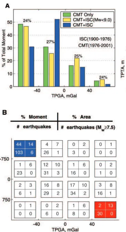
negative TPGA (Section 1.2, Fig. 1.6). To emphasize the relationship between large
earthquakes and TPGA, we consider histograms of moment release vs. TPGA, using
four bins of about equal areas of the plate interface. Seismic moment released in one
fourth of the total area with positive TPGA (>40 mGal) accounts for less than 5% of
the total moment released in the 20th century regardless of whether or not we include
the three largest earthquakes. Furthermore, the average seismic moment per event
for earthquakes occurring in areas with negative TPGA (< −40 mGal) is over ten
times larger than that for those occurring in areas with large positive TPGA (Section
1.2). We note that while great earthquakes occur predominantly in areas with large
amplitude negative TPGA, the converse relationship does not necessarily hold, i.e.,
not all regions with negative TPGA necessarily experience great earthquakes.
Using the ETOPO-5 (21) digital elevation model, we treat bathymetry in the same
manner as the gravity field to form the trench parallel topography anomaly (TPTA)
(11). Areas with strongly negative TPGA and TPTA (< −750 m) are the most
active in terms of both the number of total events and the number of large events
) Histogram of total seis-mic moment versus TPGA. We con-sider separately events only in the CMT catalog (1976 to 2001), as well as a combined set of CMT (1976 to 2001) and ISC (1900 to 1976). We only considered events 6.0. The percentage of area in each bin is shown above ) Seismic moment re-lease versus TPGA and TPTA. The number in the upper left of each cell indicates the percentage of to-tal moment associated with the corresponding range of TPGA and TPTA. The numbers at the upper right, lower left, and lower right of each cell indicate the percentage of
Figure 1.2: (A) Histogram of total seismic moment vs. TPGA. We consider separate events only in the CMT catalog 2001), as well as a combined set of CMT
(1976-2001) and ISC (1900-1976). We only consider events withMw ≥6.0. The percentage
of area in each bin is shown above each bar. (B Seismic moment release vs. TPGA and TPTA. The number in the upper-left corner of each cell indicates the percent of total moment associated with the corresponding range of TPGA and TPTA. The numbers at upper-right, lower-left, and lower-right corner in each patch indicate percent of
interface area, number of earthquakes, and number of large earthquakes (Mw ≥7.5),
TPGA and TPTA (> 750 m) are relatively quiescent.
Most remarkably, 14% of the area with strongly negative TPGA and TPTA
corre-sponds to 44% of total moment released, while equivalent areas with strongly positive
TPGA and TPTA only represent 2% of total moment. Seismic moment density
(mo-ment per unit area) in areas with strongly negative TPGA and TPTA (Fig. 2B,
Fig. 1.10, blue bin), is over 40 times that occurring in areas with strongly positive
TPGA and TPTA (Fig. 1.2B and Fig. 1.10, red bin).
Geodetic observations of strain accumulation complement inferences based on
earthquake locations by constraining the extent of coupling in a given subduction
zone. For instance, a GPS array installed in 1994 to investigate strain accumulation
in the Shumagin gap and on Kodiak Island in the Alaska-Aleutian subduction zone
indicates that Kodiak Island, a region of negative TPGA, overlies a strongly-coupled
segment of the subduction zone (22, 23) with an implied potential for large
earth-quakes (Fig. 1.1B). GPS data for the Shumagin gap, a region of positive TPGA,
shows much less strain accumulation (24, 25) and is inferred to overlie a segment of
the subduction zone that is relatively uncoupled.
Fore-arc basins off the Nankai Trough in Japan are known to coincide with the
size and spatial extents of areas of significant moment release during great
earth-quakes (26). The Kermadec subduction zone, normally considered to be relatively
aseismic, contains a spatially restricted region several hundred kilometers long, which
has experienced several large earthquakes (Fig. 1.11A). This seismically active zone
occurs within a much broader region of negative TPGA, but more importantly, as
with Nankai, it conforms to a fore-arc basin characterized by a 1.5 km increase in
sediment thickness (Fig. 1.11A) (27). Such a strong correlation between topographic
depressions and the locations of great earthquakes (28) is equivalent to the correlation
with large amplitude negative TPTA.
Along-strike variations in the position of the coastline (29) relative to the trench
can also be considered as a form of TPTA. For instance, models of co-seismic slip from
the 1995 Mw 8.1 Antofagasta earthquake (30) show that the region of significant
if slip in the seismic gap to the north (last rupture in 1877) will extend under the
peninsula, or stop just north of it. Similarly, no significant co-seismic slip is inferred
to have occurred below Cape Muroto during the 1946 Nankai earthquake (31), and
during the 1960 Chilean earthquake, co-seismic slip is inferred to have significantly
decreased before reaching the peninsula south of the city of Conception (Fig. 1.6A)
(19). The correlation of bathymetric highs with the absence of great earthquakes (32)
is equivalent to the correlation with large amplitude positive TPTA.
We find that TPGA and TPTA are positively correlated in most areas, with little
area in regions where TPTA and TPGA are uncorrelated (Fig. 1.2B, Fig. 1.10). This
correlation is expected because gravity anomalies are intrinsically tied to topographic
variations via a given compensation mechanism. Results from viscous models (4,
5), visco-elastic models (6, 7), and laboratory experiments (8) suggest that spatial
variations in the magnitude of shear tractions on the plate interface can modulate
surface topography and gravity in the fore-arc. In particular, these models indicate
that increasing shear tractions on the plate interface induce a decrease in vertical
compressive stress, thereby depressing fore-arc topography and gravity. Consistent
with these models, we interpret our observations of TPGA and TPTA as indications of
variations in shear tractions on the plate interface, with strongly negative TPGA and
TPTA associated with relatively high shear tractions, and strongly positive TPGA
and TPTA associated with relatively low shear tractions (Fig. 1.3, left panel).
Laboratory studies of the frictional behavior of sliding rock surfaces show that the
tendency for stick-slip behavior (i.e., earthquakes) increases with increasing applied
shear tractions (Fig. 1.3, right panel) (33), where shear tractions are a function of
the applied normal stress on the sliding block and the coefficient of friction on the
contact surface. The effective coefficient of friction on the plate interface is sensitive
to many factors including differences in material properties, presence or absence of
fluids, seafloor roughness, slab geometry, temperature, and contact time.
Subduction zones have been classified between two end-member groups,
Chilean-and Mariana-type (34), Chilean-and large scale inter-arc differences in seismogenic behavior
Illustration of the ob-served correlation of TPGA and TPTA with seismogenic behavior. The left panel schematically shows variations in gravity and topography due to changes in shear tractions on the plate in-terface (red line). Solid and dashed lines indicate gravity and
topography anomalies
corre-) and high-) shear tractions on the plate interface. The right panel schematically indicates changes in seismogenic behaviors with changes in shear tractions. Large shear tractions tend to produce
Figure 1.3: Left panel schematically shows variations in gravity and topography due to changes in shear tractions on the plate interface (red line). Solid and dashed lines
indicate gravity and topography anomalies corresponding to lower (τ1) and higher (τ2)
shear tractions on the plate interface. Right panel schematically indicate changes in seismogenic behaviors with changes in shear tractions. Large shear tractions tend to produce stick-slip behaviors and small shear tractions tend to produce stable-sliding behaviors.
plate (35), or normal tractions on the plate interface (36). However, our observed
correlations between smaller scale intra-arc variations in TPGA and TPTA and
seis-mogenic behavior suggest that variations in normal tractions within a given
subduc-tion zone are probably not the dominant factor. Negative TPGA and TPGA are
associated with a reduction in normal tractions, which would on its own reduce the
tendency for stick-slip behaviour. The observed correlation of negative TPGA and
TPTA with the location of great earthquakes, suggests that the implied increases in
shear tractions must be primarily due to increases in the effective coefficient of friction
as opposed to increases in normal tractions. Likewise, positive TPGA, TPTA, and
aseismic behavior are associated with relative decreases in the effective coefficient of
friction.
Based on the observed correlation of TPGA and TPTA with seismogenic behavior,
numerical modelling of fore-arc gravity and topography, and laboratory experiments
in frictional properties of material on the plate interface within a given subduction
zone are as important in controlling seismogenic behavior as those factors that differ
between subduction zones. These variations must be sufficiently large within a given
subduction zone to cause a transition between stick-slip and stable sliding behavior.
The amplitude of the variations in gravity and topography addressed here are
many orders of magnitude larger than temporal variations over the seismic cycle.
Thus, the observed spatial pattern of TPGA and TPTA must persist over time
peri-ods much longer than the typical inter-earthquake time (102−103 years) at a given
segment of a subduction zone, and great earthquakes should be observed to
consis-tently occur in areas with large amplitude negative TPGA in the fore-arc region.
Based on the observed TPGA, we make a few testable predictions for the
seismo-genic behavior of different segments of several subduction zones. We predict that the
western Shumagin gap, Unalaska gap, and western Aleutians are expected to be
ac-cumulating elastic strain at shallow depths, while the eastern Shumagin gap, western
Aleutians at depths greater than 25 km, and Kurile trench gap should have less strain
accumulation (Fig. 1.1, Fig. 1.6B). In the northern South American subduction zone,
segments between 1◦N and 8◦S show no occurrences of great earthquakes (37). Based
on the value of TPGA in this region, we would predict low elastic strain accumulation
in the northern segment (1◦N −3◦S) and higher elastic strain accumulation in the
southern segment (4◦S−8◦S) (Fig. 1.11B). Future geodetic measurements (both on
land and on the sea floor) can test our TPGA-based predictions of which seismic gaps
are accumulating elastic strain, and which are associated with relatively uncoupled
plate interfaces (38, 39).
Refining the details of the relationship between the gravity field and large
earth-quakes requires progress in several directions: (1) The simultaneous use of geodetic
observations, tsunami waveforms, and seismological data to determine the absolute
location of co-seismic slip of large subduction zone earthquakes; (2) the use of both
marine and continental gravity data accounting for sediment thickness, and local
shallow compensation effects above the plate interface; and (3) a suite of models
Figure 1.4: (A) Alaska-Aleutian (B) Kamchatka-Kurile (C) Japan (D) Nankai (E) Ryukyu (F) Izubonin-Mariana (G) Sumatra-Java (H) Tonga-Kermadec (I) Chile (J), northern South America, (K) Central America and (L) Cascadia. Average trench-normal profiles are computed using the regions as outlined.
scales of the seismic cycle to millions of years, with attention placed on the long term
topography of the fore-arc.
1.2
Supplementary Materials and Methods
1.2.1
Construction of TPGA
The choice of the along-strike extent of the region used to calculate the local average
trench-normal gravity profile is non-unique. Our choice corresponds to the regions
outlined in Fig. 1.4.
Each region incorporates at most the entire extent of a given subduction arc, and
at a minimum, the rupture zone of several great earthquakes (Fig. 1.1B, Figs. 1.4, 1.6,
path a constant distance from the trench. In general, the gradients of TPGA discussed
in this study are visible in the original free-air gravity data (compare Figs. 1.1A and
1.1B). The removal of the average trench normal profile serves to put all subduction
zone s on a more comparable footing. The resulting TPGA primarily reflects short
wavelength variations in shallow fore-arc structures (Fig. 1.1B), and can vary strongly
in directions both parallel and perpendicular to the strike of the trench. There is no
obvious systematic dependence of TPGA on the age of subducting plates or the type
of overriding plate (continental or oceanic). We have used different sub-regions to
calculate TPGA, and found very similar estimate of TPGA (Fig. 1.5).
1.2.2
Estimation of TPGA associated with subduction zone
earthquakes
Because events in the relocated ISC and Harvard CMT catalogs are treated as point
sources, we must assume a relationship between the size of the earthquake and the
area that slipped. We assume a dip-slip rectangular fault with dimensions that scale
with seismic moment and stress drop (S1). We consider extremal values of stress
drops in the range of 1-10 MPa (S2). The slip area of each event is assumed to be
square and centered on the hypocenter. If this assumption results in surpassing the
surface or down dip limit of the slab interface, the assumed area becomes rectangular,
with the slipping area extending along strike. The CMT location is determined as
the centroid of energy release and considered as the best available global dataset of
seismic moment and location. The CMT catalogue we use spans the time period from
1976 to 2001, while the relocated ISC catalogue begins in 1900. For events in the ISC
catalogue without a corresponding CMT-determined seismic moment, we estimate
moment via a moment-magnitude relationship (S3, S4).
The distribution of co-seismic slip for the three largest earthquakes may be
com-plicated and our assumed hypocenter, fault area, and computed mean TPGA, may
thus not adequately approximate reality. Therefore, for these three events, we use
Figure 1.5: (A) Alaska (B) Aleutian (C) Kamchatka (D) Kurile subduction zones, re-spectively. The average trench-normal gravity profile calculated for the region shown in the upper insets is shown in the lower insets, whose x-axis is trench-normal dis-tance in degrees and the y-axis is gravity in mGal. The color bar shows the amplitude of the free-air gravity anomaly. Subduction zone earthquakes from the ISC
(1900-1976) with Mw = 7.5 and Harvard CMT (1976-2001) catalogues with Mw = 7.0, are
1.2.3
Construction of TPTA
As with the TPGA, we bin the TPTA in four groups with equal total area in a
given range of TPTA. We note that ETOPO-5 data is not as highly resolved as the
gravity data (S8, S9). Gravity data is higher resolution with 30 sec grid spacing while
ETOPO-5 data is with 5 min grid spacing. Track lines used to construct ETOPO-5
are denser in along the convergent plate boundary (refer to Fig. 1 in S9,) the error
due to gridding is not likely to be significant at the scales of interest (several tens of
kilometers).
1.2.4
Moment release versus TPGA
We first consider the distribution of moment for individual events versus TPGA
(Fig. 1.6).
For events in either the CMT or the ISC catalogues, no great earthquakes (Mw >
8.0) occur in areas with positive TPGA (> 40 mGal). Given the large number of
events involved, we find it useful also to consider the distribution of cumulative
mo-ment (Fig. 1.7).
We observe that about 80% of the cumulative moment is produced in 30% of
total area of subduction zone with TPGA less than −30 mGal, while less than 20%
of cumulative moment is produced in the 70% of the area of subduction zone with
TPGA greater than −30 mGal. The total cumulative seismic moment is dominated
by the three largest earthquakes of the 20th century. When excluding the three
largest earthquakes, we find that about 45% of the remaining total seismic moment
is produced in about 25% of the total area of subduction zone with highly negative
145E 150E 155ûE 160E
45N 50N 55N
500 km
-40 -20 0 20 40
mGal
B
Kam cha
tka
Hokka ido
1952 Mw=9.0
gap
-200 0 200
-2.5 0.0 2.5
Kamchatka/Kurile
80ûW 75ûW 70ûW
50ûS 45ûS 40ûS 35ûS
500 km
A
-2000 200
-2.5 0.0 2.5
-200 0 200
-2.5 0.0 2.5
[image:28.612.142.507.216.467.2]Chile Conception
Figure 1.7: Solid and open circles indicate data from CMT and ISC catalogue, re-spectively. Cumulative precent of total seismic moment with respect to TPGA for the
entire ISC catalogue, ISC catalogue with Mw < 9.0, and CMT catalogue are shown
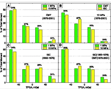
Figure 1.8: (A) All CMT events (1976-2001) with Mw = 6.0. (B) All events with
Mw = 6.0 located in both CMT and ISC catalogues (1976-2001). A 10 MPa stress
drop is assumed when estimating slip area. (C) All ISC events in 1900-1976. (D) All CMT events (1976-2001) and ISC events (1900-1976).
1.2.5
Robustness of correlation between TPGA and seismic
moment
Despite the inherent limitations of the global earthquake catalogues, such as event
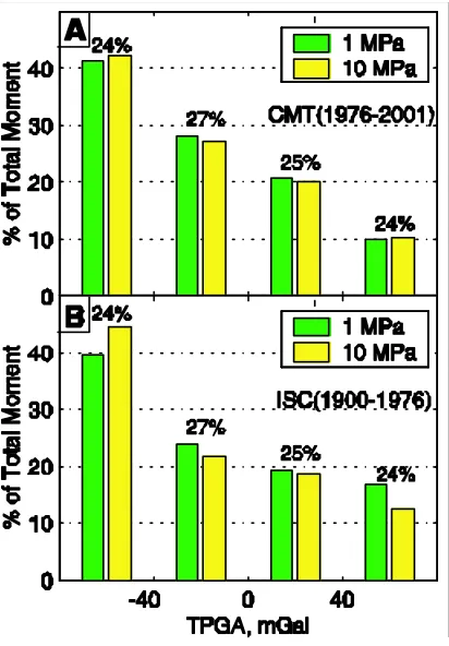
mislocation and incompleteness, the correlation between TPGA and the occurrences
of large earthquakes does not depend on the assumed magnitude of the stress drop,
which catalog is used, or how seismic moment is distributed over a given earthquake’s
fault area (Fig. 1.8 and Fig. 1.9).
In addition, Monte Carlo permutation tests (S10) indicate that the difference in
total seismic moment between areas with strongly negative TPGA (<-40 mGal) and
areas with strongly positive TPGA (> 40 mGal) is significant at a 95% confidence
Figure 1.9: Here we do not calculate the average TPGA for a given earthquake. In-stead, the plate interface is pixelated into small (about 0.1 x 0.1 deg) cells of constant TPGA, and the seismic moment for a given earthquake is evenly distributed onto the cells within the estimated fault area. We then form the histogram by evaluating the total distributed moment in cells lying within a given range of TPGA. (A) All CMT
events (1976-2001) with Mw = 6.0. (B) All ISC events from 1900-1976. The percent
1.3
References
1. B. H. Hager, R. J. O’Connell, A. Raefsky, Tectonophysics. 99, 163 (1983).
2. S. Zhong, M. Gurnis, J. Geophys. Res. 99, 15683 (1994).
3. M. I. Billen, M. Gurnis, Earth Planet. Sci. Lett. 193, 227 (2001).
4. S. Zhong, M. Gurnis, Geophys. Res. Lett. 19, 1891 (1992).
5. S. J. H. Buiter, R. Govers, M. J. R. Worterl, Geophys. J. Int. 147, 415 (2001).
6. S. Wdowinski, J. Geophys. Res. 97, 17651 (1992).
7. R. Cattin, H. Lyon-Caen, J. Chery, Geophys. Res. Lett. 24, 1563 (1997).
8. Shemenda, A. I. in Subduction: insight from physical modeling, Modern
ap-proaches in Geophysics, vol. 11, 215pp (1994).
9. D. T. Sandwell, W. Smith, J. Geophys. Res. 102, 10039 (1997).
10. We restrict ourselves to this global dataset to maintain geographic uniformity of
the analysis. This restriction implies that we consider only TPGA in offshore areas.
11. Materials and methods are in Section 1.2.
12. We note that the subduction interface can be conveniently classified using TPGA
into four about equal area bins associated with the TPGA ranges of less than -40
mGal, -40 to 0 mGal, 0 to 40 mGal and greater than 40 mGal, respectively.
13. A. M. Dziewonski, T. A. Chou, J. H. Woodhouse, J. Geophys. Res. 86, 2825
(1981).
14. E. R. Engdahl, D. R. Van der Hilst, R. P. Buland, Bull. Seis. Soc. Am. 88, 722
(1998).
15. When using these catalogs, we attempt to use only fore-arc thrust events between
0 and 50 km depth in the Benioff zone, where the plate interface is probably coupled.
16. L. Ruff, H. Kanamori, Phys. Earth Planet. Inter. 31, 202 (1983).
17. J. Johnson, Adv. in Geophys. 29, 1 (1998).
18. S. Beck, D. H. Christensen, J. Geophys. Res. 96, 2205 (1991).
19. S. E. Barrientos, S. N. Ward, Geophys. J. Int. 103, 589 (1990).
20. J. M. Johnson, K. Satake, Pure Apply. Geophysics. 154, 541 (1999).
Data Announc. 88-MCG-02, Natl. Oceanic and Atmos. Admin. U. S. Dept.
Com-mer., Boulder, Colo. (1988).
22. H. J. Fletcher, J. Beavan, J. Freymuller, L. Gilbert, Geophys. Res. Lett. 28, 443
(2001).
23. C. J. Zweck, J. Freymuller, S. C. Cohen, J. Geophys. Res. 107, 10.1029/2001JB000409
(2002).
24. K. M. Larson, M. Lisowski, Geophys. Res. Lett. 21, 489 (1994).
25. J. T. Freymuller, J. Bevan, Geophys. Res. Lett. 26, 3233 (1999).
26. Y. Sugiyama, Geofisica Internacional 33, 53 (1994).
27. National Geophysical Data Center, Total Sediment Thickness of the World’s
Oceans & Marginal Seas, Natl. Oceanic and Atmos. Admin. U. S. Dep. Commer.,
Boulder, Colo. (1996).
28. K. Mogi, Bull. Earthquake Res. Inst. 47, 429 (1969).
29. L. Ruff, B. W. Tichelaar, What controls the seismogenic plate interface in
sub-duction zones? Subsub-duction: Top to Bottom, AGU Geophysical Monograph Volume
96, edited by Gray E. Bebout, David W. Scholl, Stephen H. Kirby, and John P. Platt,
pp. 105-111 (1996).
30. M. E. Pritchard, M. Simons, M., P. A. Rosen, S. Hensley, F. H. Webb, Geophys.
J. Int. 150, 362 (2002).
31. Y. Tonioka, K. Satake, Earth Planet Space 53, 235 (2001).
32. J. Kelleher, W. McCann, J. Geophys. Res. 81, 4885 (1976).
33. C. Marone, Annu. Rev. Earth Planet. Sci. 26, 643 (1998).
34. S. Uyeda, H. Kanamori, J. Geophys. Res. 84, 1049 (1979).
35. H. Kanamori, Annu. Rev. Earth Planet. Sci. 14, 293 (1986).
36. C. H. Scholz, J. Campos, J. Geophys. Res. 100, 22103 (1995).
37. T. Lay, H. Kanamori, L. Ruff, Earthquake Pred. Res. 1, 1 (1982).
38. S. P. Nishenko, Pure Apply. Geophys. 135, 169-259 (1991).
39. Y. Y. Kagan, D. Jackson. J. Geophys. Res. 100, 3943-3959 (1995).
40. National Geophysical Data Center, Global Relief data (CD-ROM). World Data
41. O. Gudmundsson, M. Sambridge, J. Geophys. Res. 103, 7121 (1998).
42. C. DeMets, R. G. Gordon, D. F. Argus, Geophys. Res. Lett. 21, 2191 (1994).
S1. T. Lay, T. Wallace, in Modern Global Seismology, 521pp (1995).
S2. H. Kanamori, D. L. Anderson, Bull. Seis. Soc. Am. 65, 1073-1095 (1975).
S3. P. Chen, H. Chen, Tectonophysics, 166, 53-72 (1989).
S4. H. Kanamori, Tectonophysics, 93, 185-199 (1983).
S5. L. Ruff, H. Kanamori, Phys. Earth Planet. Inter. 31, 202 (1983).
S6. S. E. Barrientos, S. N. Ward, Geophys. J. Int. 103, 589 (1990).
S7. J. M. Johnson, K. Satake, Pure Apply. Geophysics. 154, 541 (1999).
S8. National Geophysical Data Center, ETOPO-5 bathymetry/topography data,
Data Announc. 88-MCG-02, Natl. Oceanic and Atmos. Admin. U. S. Dep.
Com-mer., Boulder, Colo. (1988).
S9. W. H. F. Smith, J. Geophys. Res. 98, 9591 (1993).
S10. E. L. Lehmann, in Testing Statistical Hypothesis. Wiley publications in
statis-tics, 369 pp (1959).
S11. National Geophysical Data Center, Global Relief data (CD-ROM). World Data
Center for Marine Geology and Geophysics, Boulder, Colo. (1993).
S12. O. Gudmundsson, M. Sambridge, J. Geophys. Res. 103, 7121 (1998).
S13. C. DeMets, R. G. Gordon, D. F. Argus, Geophys. Res. Lett. 21, 2191 (1994).
S14. S. E. Barrientos, S. N. Ward, Geophys. J. Int. 103, 589 (1990).
S15. T. Lay, H. Kanamori, L. Ruff, Earthquake Pred. Res. 1, 1 (1982).
S16. J. M. Johnson, K. Satake, Pure Apply. Geophysics. 154, 541 (1999).
S17. L. Ruff, H. Kanamori, Phys. Earth Planet. Inter. 31, 202 (1983).
S18.National Geophysical Data Center, Total Sediment Thickness of the World’s
Oceans & Marginal Seas, Natl. Oceanic and Atmos. Admin. U. S Dep.
Chapter 2
Excitation of Earth’s Free
Oscillations by the 26 December
2004 Sumatra-Andaman
Abstract
At periods greater than 1000 sec, Earth’s free oscillations excited by the 26
De-cember 2004 great Sumatra-Andaman earthquake have anomalously large amplitude
when referenced to the Harvard CMT fault mechanism (1), which is estimated from
300−500 sec surface waves (2). On a steeper fault with a time-dependent rupture
model that matches seismic body and surface waves in greater detail (3), free
oscilla-tion amplitudes can be approximated with a seismic moment (Mo = 6.5×10²² N-m)
that corresponds to moment-magnitude Mw = 9.15, close to the geometric mean of
initial estimates from surface waves (Mw = 9.0) and the mode 0S2 (Mw = 9.3). With
a rupture duration τ = 600 seconds, the fault-rupture models do not represent well
geodetic observations. It argues for larger fault displacement beneath the Nicobar and
Andaman Islands (4). As a second author of this paper, I have contributed to most
of the source modeling and figures (Fig. 2.2, Fig. 2.3A, Fig. 2.4, Fig. 2.6-Fig. 2.8).
2.1
Introduction
The 26 December 2004 Sumatra-Andaman earthquake delivered a hammer blow to
our planet, exciting a plethora of vibrational free oscillations that, at periods T>1000
s, remained observable for weeks in broadband seismic data from global networks. The
frequencies and decay rates of Earth’s free oscillations offer strong constraints on our
planet’s interior composition, mineralogy, and dynamics (5−14), so analysis of
long-period seismic data from this event should offer new perspectives on Earth structure.
In this report we discuss how seismic free oscillations also provide information on the
remarkable size and duration of this earthquake.
Because Earth is approximately spherical, the geographical patterns of its free
vibrational modes can be expressed in terms of the angular harmonics Ylm(θ, φ) and
their vector gradients, where l is the angular degree, m is the azimuthal order, θ is
colatitude and φ is longitude. On a simple spherical planet (15), the free oscillations
follow either a spheroidal (S) or toroidal (T) vibrational pattern and have
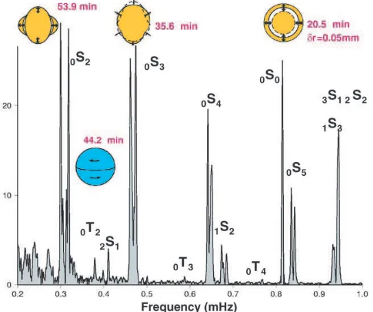
spectro-scopic notation nSlm and nTlm, where n is the radial overtone number (Fig. 2.1).
For a spherical reference model, all 2l+1 vibrations ofnSlmandnTlm, have identical
frequency. On the real Earth, departures from the symmetries of a spherical reference
model cause its free oscillations to couple, hybridize and suffer fine-scale splitting of
their vibrational frequencies (16−19). Frequency splitting of free oscillations with
periods T>1000 s is caused mainly by Earth’s rotation, similar to Zeeman splitting
of electron energies in an external magnetic field (20, 21).
Earth’s free oscillations were first reported after Fourier analysis of hand-digitized
analog seismic records of the megathrust earthquakes of the middle 20th century
(22-25), particularly the 22 May 1960 Chilean earthquake (Mw = 9.5). These huge
events saturated most seismometers of the time, rendering many hours of data
un-usable. Frequency estimates from smaller, deeper earthquakes, more amenable to
hand-digitization and Fourier analysis, led to accurate spherical-reference models for
our planet’s interior (5). Detailed study of free oscillation attenuation, frequency
behavior is readily observable for mode pairs nearly 200 km. The relative excitation of the
Figure 2.1: Schematic of the motion of free oscillations 0S2, 0T2, 0S3 and 0S0,
and by the advent of the Federation of Digital Seismic Networks (FDSN) with
high-dynamic range induction-feedback sensors capable of recording faithfully the seismic
waves from great earthquakes (28).
2.2
Broadband seismography data
The 2004 Sumatra-Andaman earthquake tested broadband seismographic technology
on a global scale. Peak ground motions exceeded 1 cm at all locations on Earth’s
solid surface (29). In one portion of the FDSN, 88% of the 125 stations of the Global
Seismographic Network (GSN), operated directly by the U. S. Geological Survey and
the IDA Project of the University of California, San Diego (30), recorded data without
interruption or distortion (31). Stations of the Geoscope network (32) had similar
success.
In all, data records from more than 400 FDSN stations were of sufficient quality to
observe Earth’s free oscillations with unprecedented signal-to-noise ratios. A broad
distribution of stations facilitates using Ylm(θ, φ)-weighted stacks of data spectra to
isolate individual Earth vibrations (Fig. 2.10, Section 2.5). The recent installation
of a broadband seismometer in the South Pole Quiet Zone provides natural isolation
of the m = 0 singlets of long-period modes (Fig. 2.2).
Free oscillations can also be sought in complementary observations (Fig. 2.3) from
strainmeters and tiltmeters (33-35), from superconducting gravimeters (36-38), and
from continuously-recording GPS receivers (39,40). Superconducting gravimeter data
offers an important calibration for seismometer data at periods T>1000 s (41). The
amplitude of the ”breathing mode” 0S0 is geographically constant to high accuracy;
station-by-station comparisons of its amplitude in data from the IDA network suggest
that a significant minority of seismometers suffer 5-10% deviations from their nominal
responses (31).
The largest earthquakes offer the most penetrating and long-lasting seismic probes
of Earth’s deep interior, revealing behavior predicted by theory, but only rarely
Free-oscillation spectra for GSN station QSPA, whose sensor lies within an ice borehole in the quiet sector of the South Pole station. Only 0 free oscillations are nonzero at Earth’s poles, lead-ing to sharply defined slead-ingle resonance peaks for modes
9
1000 s. A vertical-motion data series of 106 hours was analyzed. Predicted spectra are plotted with colored lines
from Harvard CMT mechanism and two finite rupture models from (4).
0.2 0.3 0.4 0.5 0.6 0.7 0.8 0.9 1 0
1 2
x 10-6
|r • a(x, ω ) | Frequency, mHz QSPA model II model III CMT
0S2 0S4 0S0
0S3
0S5 1S2
Figure 2.2: Free-oscillation spectra for GSN station QSPA, whose sensor lies within an ice borehole in the Quiet Sector of the South Pole Station. Only m=0 free oscillations are nonzero at Earths poles, leading to sharply-defined single resonance peaks for
modesnSlandnTl with period T>1000 s. A vertical-motion data series of 106 hours
was analyzed.
associated with Earth’s Coriolis force causes them to form hybrid vibrational
pat-terns. The hybridized toroidal modes are predicted to acquire a vertical vibrational
component, a feature nominally restricted to spheroidal modes. Although this
behav-ior is readily observable for mode pairs 0Sl−0Tl+1 in the 300-500 s period range that
are close in frequency (26,27), at frequencies below 1 mHz the coupling is weaker and
was not observed with seismometers before the 2004 Sumatra-Andaman earthquake
(Fig. 2.1, ref. 42 and Fig. 2.11 in section 2.5).
The geometry of low-degree modes allows us to constrain the long-period centroid
of the earthquake (7,22). For a centroid at the equator, excitation of the m ± 1
vibrations of the mode 0S2 would be zero for an earthquake on the east-dipping
Sumatra-Andaman thrust fault. The amplitude of the m=−1,+1 vibrations, of 0S2
relative to them=−2,0, and +2 vibration, indicates how far northward the
Sumatra-Andaman earthquake ruptured (Fig. 2.4). The event hypocenter and CMT location lie
at 3.2◦N and 3.1◦N, respectively, displaced east-west by nearly 200 km. The relative
excitation of the m = ±1 vibrational modes of 0S2 is significantly underpredicted
by this location centroid. Better agreement is obtained for a seismic source centroid
closer to 7.5◦N, suggesting a source process that extends into the northern half of the
slip motion as the rupture progressed north ); modeling suggests that the northern third of the fault zone contributed little to the ob-). Many factors suggest that fault motion was larger and faster in the south of the fault zone, where rupture began, and
Drawing on infer-ences made from these data, we consider here two finite-rupture models based on body and in which rupture has longer duration (600 s ver-sus 300 s), longer length (1300 km verver-sus
0.280 0.34
0.2 0.4 0.6 0.8
1x 10
-6
Frequency, mHz
0
S
2|r • a(x, ω )| Data CMT x 2.6 CMT (7.5°N) x 2.6
m = -1 m = 1 m = -2
m = 2
Figure 2.4: Black: data. Red: prediction for the Harvard CMT mechanism and
location but at 2.6 times larger scalar moment. Note how the m = 1 and m = −1
singlets are too small, indicating that the CMT centroid is too close to the equator. Green: prediction from 2.6 times the CMT moment but with a centroid location at
7.5◦N, which improves the fit to the m = 1 and m = −1 singlets. A Hann taper
has been applied to the 144-hour time series starting from the origin time of this earthquake.
2.3
Earthquake size and duration
Since the late 1970s seismologists have estimated magnitudeMw for large earthquakes
in terms of the seismic moment Mo (46). As a measure of the average displacement
integrated over the ruptured fault zone, seismic moment Mo is associated with its
zero frequency behavior. It is therefore logical to estimate Mo from the amplitudes
of the gravest Earth free oscillations, such as the modes 0S2, 0S3, 0S4, 0S0, and 1S0.
For nearly all earthquakes these modes are excited too weakly for direct observation,
but the Sumatra-Andaman event was different. The “football mode” 0S2, the free
oscillation with the longest observed period (54 minutes), is expressed strongly in
vertical-component spectra computed from a large proportion of individual stations,
as are many of the shorter-period modes. The amplitudes of several spheroidal free
oscillations with periods T >1000 s were a factor of 1.25 to 2.6 larger than predicted
by the Harvard CMT source (1,2), reaching a maximum for the mode 0S2 (Fig. 2.4
and Fig. 2.5).
solution, i.e., thrusting on a shallow-dipping fault (8◦ dip), the estimated earthquake
magnitude Mw increases from 9.0 to 9.3.
Source spectral amplitude is larger at long period for earthquakes with long time
duration. If seismic rupture progresses at a constant rate for a finite duration τ,
from a sharp onset to an equally abrupt termination, the source spectrum M(f) =
M o(sinπf τ)/(πf τ) a function of cycle frequency f (47). The logarithm of M(f)
exhibits a low-frequency plateau that transitions to a power-law slope at a corner
frequency fc = πτ1 . Fig. 2.5 graphs the source spectra implied by several spheroidal
modes against M(f) source spectra for constant-rupture durations τ = 800 s and
τ = 320 s. Modal amplitudes do not follow the predictions of a constant-rate source
spectrum, suggesting a variable rupture-propagation rate. For example, the rupture
of two large fault segments with different orientations, onset times and durations
would cause spectral interference at long period. Such complexity aside, the trend of
modal amplitudes is consistent with a rupture duration τ ≤800 s.
The initial phase of0S0, relative to the earthquake onset, supports the inference of
long source duration,τ. The initial phase of a free oscillation of period, T, aligns with
the time centroid of the rupture process if the rupture duration is relatively small,
i.e., τ T. Phase cancellation damps the modal excitation if τ ≥ T /2, and the
relation of modal initial phases with the source time centroid becomes complicated.
We estimate the initial phase of0S0 to average 65◦−66◦ in the Global Seismographic
Network and to average 61◦ over ten records from the Geoscope network (Fig. 2.12).
The initial displacement of 0S0 is positive (0◦ phase), so this suggests a time centroid
delayed 205 to 225 s relative to the earthquake onset. Rupture duration τ would be
between 400 and 450 s if rupture rate were constant. The initial phase of 1S0 is 115.7◦
averaged for ten Geoscope stations, consistent with a time centroid of 197 s. Variable
rupture rate will cause scatter in time centroids estimated from different modes.
Free-oscillation observations constrain the Sumatra-Andaman earthquake source,
but the constant-rupture model is too simple. A complex earthquake process is
sug-gested by a number of observations, e.g., large bursts of high-frequency seismic
m) than that inferred from the CMT solution (Fig. 6). Both models pre-scribe a spatially varying fault geometry that is, on average, steeper than the CMT solution. A steeper fault is more efficient at exciting the long-period modes, and therefore the finite rupture models can greatly improve the match between predicted and observed modal ampli-than in-). A transition to oblique thrust motion in the Andaman islands region im-proves the fit to long-period toroidal modes. Model III, which prescribes a peak rate of rupture propagation somewhat earlier than model II, is slightly more successful at pre-dicting the absolute value of modal vertical-component spectral peaks, typically with an average misfit pf less than 10%, depending on the mode (Figs. 2, 7, and 8 and table S1). Despite the rough success of a single seismic rupture model across the entire seismic
spec-CMT Moment
320-s Duratio n 800-s Duratio
n
0S2
1.0
1.5
2.0
2.5
3.0
Source Si
z
e Relati
ve to CMT
0.4
0.8
1.2
1.6
Frequency (mHz)
0S3
0S4 0S0
1S0
Figure 2.5: The measured amplitudes of several long-period free oscillations, ex-pressed in terms of the seismic moment required for excitation by the shallow-thrust fault geometry of the Harvard CMT solution. Crosses indicate free oscillation am-plitudes measured on data from GSN stations; triangles are estimated independently using data from Geoscope stations. The largest amplification is associated with the
mode 0S2, whose apparent moment is roughly 2.6 times the CMT moment estimated
segment of plate margin (4), but in the northern 400 km of the zone the aftershocks
commence some 85 minutes after rupture onset (49); substantial surface wave
direc-tivity at periods approaching 1000 s (3); the dip of the Sumatra-Andaman megathrust
in its northern half tends to exceed the 8◦ dip of the Harvard CMT source mechanism
(4); back-arc spreading in the Andaman Sea may have promoted the expression of
strike-slip motion as the rupture progressed north (4); modeling suggests that the
northern third of the fault zone contributed little to the observed tsunami (4). Many
factors suggest that fault motion was larger and faster in the south of the fault zone,
where rupture began, and was smaller and slower in the north.
2.4
Modeling the rupture
Drawing on inferences made from these data, we consider here two finite-rupture
models based on body and surface waves (Models II and III of reference 3) in which
rupture has longer duration (600 s versus 300 s), longer length (1300 km versus 400
km) and larger moment (6.5×10²²N-m versus 4.0
×1022N-m) than inferred from the
CMT solution (Fig. 2.6).
Both models prescribe a spatially varying fault geometry that is, on average,
steeper than the CMT solution. A steeper fault is more efficient at exciting the
long-period modes, and therefore the finite rupture models can greatly improve the
match between predicted and observed modal amplitudes with a far smaller seismic
momemt (Mo) than inferred by (2). Model III, which prescribes a peak rate of
rupture propagation somewhat earlier than Model II, is more successful at predicting
the absolute value of modal vertical-component spectral peaks, typically with average
misfit less than 10%, depending on the mode (Fig. 2.7 and Table 2.1 in section 2.5).
Despite the rough success of a single seismic rupture model across the entire
seismic spectrum, geodetic evidence for a slow component of Sumatra-Andaman
dis-placement cannot be dismissed. Fault slip of ∼ 1 hour in duration, as suggested
by tsunami modeling for the Nicobar-Andaman fault segment (4), would excite
of Sumatra-Andaman displacement cannot be 1 hour in duration, as suggested by tsunami modeling for the Nicobar-), would excite seismic free oscillations inefficiently because of phase cancellation. Its signature would be expressed as a complex pattern of modal am-plitude and phase anomalies. Modal spectra for the 2004 Sumatra Andaman earthquake are more difficult to predict with simple param-eterized rupture models than modal spectra from the 28 March 2005 northern Sumatra 8.6), despite higher signal-to-noise ratios in the larger event (Fig. 8). If amplitude and phase misfits leave unexplained 10% or more of the long-period free-oscillation amplitudes of the 2004 event, slow fault 8.4 would
0 200 400 600
0 1 2 3 4 x 10
20
Time from event onset [sec]
Moment
rate function [N
e
wton-m/sec]
model II model III CMT
Figure 2.6: Moment-rate functions (MRFs) for the 26 December Sumatra-Andaman earthquake. The MRF associated with the Harvard CMT is given by the green line, the MRF of finite-fault inversion II of (3) is denoted by the blue line, and the MRF of finite-fault inversion III of (3) is denoted by the red line.
Comparison of data (NNA, at Nana, Peru) and synthetics from vari-ous models. Low-order spheroidal
at vertical component at
hori-top).
A Hann taper is applied to 144-hours time series of vertical motion before discrete Fourier transforma-tion. Similar tapering was performed on 44-hour time series of radial and transverse horizontal motion before
0.280 0.34
0.5 1 1.5x 10
?6 0S2
Frequency, mHz |r • a(x, ω )| Vertical motion NNA model (II) model (III) CMT
0.440 0.5
1 2x 10
-6
Frequency, mHz
0.550 0.62
1 2 3 |r • a(x, ω )| Frequency, mHz
0.730 0.8
2 4
Frequency, mHz
0.550 0.62
0.5 1 1.5
Frequency, mHz
0.730 0.8
0.5 1 1.5 Frequency, mHz Vertical motion Radial motion Radial motion Transverse motion Transverse motion
x 10-6 x 10-6
x 10-6 x 10⁻⁶
0S3
0T3 0T4 0T3 0T4
Figure 2.7: Comparison of data (NNA, at Nana, Peru) and synthetics from various
models. Low order spheroidal modes 0S2, 0S3 at vertical component and toroidal
modes0T3,0T4 at horizontal component are shown above. A Hann taper is applied to
S p e c t r u m comparison for the 26 December 2004 Sumatra-Andaman and 28 March 2005 Northern Sumatra earthquakes using 127-hour records of vertical motion recorded at sta-tion KMBO (Kilima Mbogo, Kenya). Spec-tral predictions of the Harvard CMT solutions are graphed as well as spectra predicted from finite-rupture ). Note the greater success of the CMT solution for the 2005 event, con-sistent with a smaller less complex rupture
0.3 0.4 0.5 0.6 0.7 0.8 0.9 1
0 2 4
x 10-6 2004 Sumatra-Andaman
|r • a(x, ω )| KMBO model II model III CMT
0.3 0.4 0.5 0.6 0.7 0.8 0.9 1
0 2 4
2005 Northern Sumatra
Frequency, mHz |r • a(x, ω )| KMBO model II model III CMT
0S2
0S0 0S4
0S3
0S5
1S2 0S2
0S0 0S4
0S3
0S5
1S2
x 10-7
Figure 2.8: Spectrum comparison for the 26 December 2004 Sumatra-Andaman and 28 March 2005 Northern Sumatra earthquakes, using 144-hour records of vertical motion recorded at station KMBO (Kilima Mbogo, Kenya). Spectral predictions of the Harvard CMT solutions are graphed, as well as spectra predicted from finite-rupture models from (3). Note the greater success of the CMT solution for the 2005 event, consistent with a less complex rupture process.
expressed as a complex pattern of modal amplitude and phase anomalies. Modal
spectra for the 2004 Sumatra-Andaman earthquake are more difficult to predict with
simple parameterized rupture models than modal spectra from the 28 March 2005
Northern Sumatra earthquake (Mw = 8.6), despite higher signal-to-noise ratios for
the larger event (Fig. 2.8). If amplitude and phase misfits leave unexplained 10%
or more of the long period free-oscillation amplitudes of the 2004 event, slow fault
motion equivalent to magnitude at least Mw = 8.4 would be possible, a geophysical
event itself larger than any earthquake between 1965 and 2001.
For both Sumatran earthquakes, modal amplitude and phase anomalies will
con-strain any additional long-term slip. In this context, the calibration and long-term
resilience of global seismographic networks is paramount. A future megathrust
earth-quake (Mw ≥9.0) is inevitable somewhere along Earth’s plate boundaries, but may
not occur for a decade or more, after today’s seismometers have begun to age and
seis-mographic networks, the Streckeisen STS-1 (52), is no longer manufactured. It is
important for the international seismological community to consider designing the
next-generation broadband seismic sensor.
2.5
Supplementary material
Here we present some graphical material to complete the exposition of the main
manuscript.
A Note on Mode Coupling at Periods T<1000 s. The largest earthquakes offer the
most penetrating and long-lasting seismic probes of Earth’s deep interior, revealing
behavior predicted by theory, but only rarely observed above ground noise. The
coupling between spheroidal and toroidal modes associated with Earth’s Coriolis force
causes them to form hybrid vibrational patterns. The hybridized toroidal modes are
predicted to acquire a vertical vibrational component, a feature nominally restricted
to spheroidal modes. Although this behavior is readily observable for mode pairs 0Sl
0Tl+1 in the 300-500-s period range that are close in frequency (26,27), at frequencies
below 1 mHz the spectral separation between modes is quite large and the coupling
effects are weaker and more difficult to observe. Furthermore, the instrumental
self-noise of the broad-band seismometers used in global seismic networks increases at
low frequencies. Earths gravest free oscillations have therefore been studied primarily
with gravimeter records, not seismometer records, after correction for fluctuations in
atmospheric pressure (42-45). The signal-to-noise ratio for seismometer records of
the 23 June 2001 Peru event (until Sumatra-Andaman the largest digitally recorded
earthquake) was not high enough to allow the observation of hybridized toroidal
modes on the vertical components. Such vertical motion has been reported previously
from a gravimeter record. Vertical components of the toroidal modes0T3 and0T4were
observed after the strike-slip Mw = 8.2 1998 Balleny earthquake (27). This was only
possible after correction for atmospheric pressure effects. The mode 0T2 was not
Figure 2.9: Schematic illustration of some simple free oscillations, superimposed on a spectrum computed from superconducting gravimeter data collected in Canberra, Australia, near station CAN of the Geoscope Network. A 240-hr record of vertical acceleration is analyzed.
Figure 2.10: Gilbert and Dziewonski (5) showed that spectrum estimates from a global network could be summed with spherical-harmonic weights to enhance signal-to-noise ratios for specific Earth free oscillations. A further processing step, called ”stripping”, isolates modal spectral peaks associated with a single spherical harmonic.
For the 2004 Sumatra-Andaman earthquake, the modes 0S2, 0S3, 0S4 and 1S2 were
observed with an unprecedented signal-to-noise ratio. The mode pair 1S3/3S1 has
been observed with similar quality most recently during the 4 October 1994 Kuril Island earthquake which, until the great 21 June 2001 Peru earthquake, was the largest earthquake since the 19 August 1977 Sumbawa earthquake. Though its source was shallow, the 2004 Sumatra-Andaman earthquake also excited inner core sensitive
Figure 2.11: Vertical seismometer amplitude spectra of 58-hour time series from five stations of global seismic networks (HKT.IU: Hockley, Texas; LVC.GE: Limon Verde, Chile; MDJ.IC: Mudanjiang, China; UNM.G: Unam, Mexico; YSS.IU: Yuzhno Sakhalinsk, Russia). The spectral peaks at the frequencies of spheroidal modes are about ten times larger than peaks at the frequencies of toroidal modes, and have been clipped for better display. Earths Coriolis force induces the toroidal and spheroidal modes to hybridize, leading to vertical motion at the frequencies of toroidal modes, obeerved well above the noise floor.
Mode Type CMT Model II Model III
0S2[0.295−0.325mHz] 0.655±0.025 0.005±0.062 0.094±0.057
0S3[0.455−0.480mHz] 0.603±0.032 −0.054±0.067 0.056±0.057
0S4[0.635−0.660mHz] 0.534±0.069 −0.158±0.117 −0.030±0.100